An algorithm for computing the gene tree probability under the multispecies coalescent and its application in the inference of population tree

Abstract

Motivation: Gene tree represents the evolutionary history of gene lineages that originate from multiple related populations. Under the multispecies coalescent model, lineages may coalesce outside the species (population) boundary. Given a species tree (with branch lengths), the gene tree probability is the probability of observing a specific gene tree topology under the multispecies coalescent model. There are two existing algorithms for computing the exact gene tree probability. The first algorithm is due to Degnan and Salter, where they enumerate all the so-called coalescent histories for the given species tree and the gene tree topology. Their algorithm runs in exponential time in the number of gene lineages in general. The second algorithm is the STELLS algorithm (2012), which is usually faster but also runs in exponential time in almost all the cases.

Results: In this article, we present a new algorithm, called CompactCH, for computing the exact gene tree probability. This new algorithm is based on the notion of compact coalescent histories: multiple coalescent histories are represented by a single compact coalescent history. The key advantage of our new algorithm is that it runs in polynomial time in the number of gene lineages if the number of populations is fixed to be a constant. The new algorithm is more efficient than the STELLS algorithm both in theory and in practice when the number of populations is small and there are multiple gene lineages from each population. As an application, we show that CompactCH can be applied in the inference of population tree (i.e. the population divergence history) from population haplotypes. Simulation results show that the CompactCH algorithm enables efficient and accurate inference of population trees with much more haplotypes than a previous approach.

Availability: The CompactCH algorithm is implemented in the STELLS software package, which is available for download at http://www.engr.uconn.edu/ywu/STELLS.html.

Contact: ywu@engr.uconn.edu

Supplementary information: Supplementary data are available at Bioinformatics online.

1 Introduction

Consider n gene lineages sampled from one population. When we trace these lineages backward in time, sooner or later two of these lineages will find a common ancestor. When this occurs, we say these two lineages coalesce or the coalescent of these two lineages occurs. Gene lineages coalesce in a stochastic way, which is influenced by multiple population genetic parameters, such as population sizes. Therefore, coalescents may potentially reveal important aspects of population evolution. In 1982, Kingman (1982) introduced the coalescent theory, which provides the analytical foundation for the study of coalescents. Since then, coalescent theory has quickly become a very active research subject in population genetics. There are numerous theoretical results in coalescent theory, along with many coalescent-based software tools. See Wakeley (2008) and Hein et al. (2005) for an overview of the growing field of coalescent theory.

While mathematically appealing, coalescent is known to be challenging computationally. One of the most important problems on coalescents is computing the coalescent likelihood. That is, we want to compute the probability of observing some population variation data under a coalescent model. However, coalescent likelihood is well known to be difficult under most formulations [see e.g. Hein et al., 2005; Wakeley, 2008]. At present, there are few polynomial time algorithms for computing coalescent likelihood except under very restricted conditions. Almost all existing approaches for coalescent likelihood computation are based on statistical techniques such as Markov chain Monte Carlo (MCMC) or importance sampling (Wakeley, 2008). These statistical approaches can be very useful in practice. However, from the computational point of view, these approaches cannot compute the exact coalescent likelihood. Moreover, approaches using MCMC tend to be very slow. Since coalescent likelihood is usually used in the inference of population evolution, accurate and efficient coalescent likelihood computation is highly desirable.

Since the work by Kingman (1982), the basic coalescent has been extended to address more aspects of population evolution. The multispecies coalescent is one such extension, and is the focus of this article. Multispecies coalescent concerns the coalescents among gene lineages from multiple populations where coalescents may cross the population boundary. Multispecies coalescent is fundamental to population evolution (Degnan and Salter, 2005; Rosenberg, 2002). Multispecies coalescent has also found applications in other domains, such as species tree inference [see, e.g. Heled and Drummond, 2010; Mirarab et al., 2014; Wu, 2012].

A key computational problem on multispecies coalescent is the computation of the gene tree probability (Degnan and Salter, 2005; Wu, 2012, 2015). Here, we are given a gene tree topology (without branch lengths) and a species tree (with branch lengths in the standard coalescent units). Note that the gene tree may not be bifurcating and there can be more than one gene lineages for a population (or taxon) in the gene tree. The gene tree probability is the probability of the gene tree topology as a result of the multispecies coalescent within the given species tree. There are only two existing algorithms for the exact gene tree probability computation. The first such algorithm is due to Degnan and Salter (2005). However, their algorithm has the exponential running time and there are no known cases of species and gene trees for which their algorithm runs in polynomial time. A much faster algorithm is given in Wu (2012), which is implemented in the program STELLS. However, the STELLS algorithm computes the gene tree probability in polynomial time only for some very special types of gene trees and species trees. We are not aware of any statistical approaches for computing the gene tree probability. The closest related approach is the MCMC approach in Heled and Drummond (2010), which is also based on multispecies coalescent. However, the likelihood computed in Heled and Drummond (2010) is for DNA sequences, not for gene trees.

In this article, we present a new algorithm, called CompactCH, for computing the exact gene tree probability. The main advantage of CompactCH is that it runs in polynomial time for any gene tree topologies and species trees when the number of taxa (populations) is fixed to be a constant. That is, the CompactCH algorithm is efficient for gene tree topologies with large number of gene lineages if the number of populations is small (i.e. there can be many gene lineages from each population). Note that although the number of gene lineages in many phylogenetic studies tends to be relatively small, the number of gene lineages in large-scale genetic studies can be large. Therefore, CompactCH may become more useful when more gene lineages are sampled from a population which is the case in genetic projects such as the 1000 Genomes Project (2015). To the best of our knowledge, CompactCH is the first algorithm for computing the gene tree probability in polynomial time that allows arbitrary gene trees and species trees when the number of populations is fixed to a constant. Note that if gene tree topologies are considered to be observed, then the gene tree probability is the likelihood of the observed gene tree topologies given the species (population) tree. In this regard, the coalescent likelihood of gene tree topologies can be computed in polynomial time under the assumption of small number of populations. We show through theoretical analysis and empirical simulations that CompactCH outperforms the existing STELLS algorithm when the number of populations is small and the gene tree contains multiple gene lineages (alleles) per taxon. We also present a new method for the inference of population divergence history (called the population tree) from large population samples, which is based on the CompactCH algorithm.

2 Background

2.1 Multispecies coalescent and incomplete lineage sorting

In this article, we use population and species interchangeably. Multispecies coalescent process (or just multispecies coalescent) concerns the coalescents of gene lineages that may occur outside the species boundary. See Figure 1 for an illustration. Multispecies coalescent lies at the intersection of population genetics and phylogenetics, and has been widely used in phylogenetic and population inference [see e.g. Heled and Drummond, 2010; Wu, 2012]. We use a rooted bifurcating tree T_s (with branch lengths) to represent the population divergence history. We use a rooted tree topology T_g to represent the genealogical history of gene lineages at a single locus. It is important to note that T_g does not have branch lengths. Also T_g may be multifurcating if the gene genealogy cannot be fully determined from the given genetic data. A common observation is that T_s and T_g do not always have the same topology. This phenomenon is called incomplete lineage sorting. We define the gene tree probability to be the probability of observing T_g for a given T_s under the multispecies coalescent model. Computing the probability of gene genealogies under multispecies coalescent is central both to phylogenetic inference of a species (or population) tree and to population genetic inference of gene flow between populations [e.g. Degnan and Salter, 2005; Heled and Drummond, 2010; Hudson, 1983; Rosenberg, 2002; Wu, 2012, 2015]. When T_s and T_g are small, simple closed-form formulas are known to calculate the gene tree probability (Hudson, 1983; Rosenberg, 2002; Takahata and Nei, 1985). When T_g and T_s become larger, computation by hand is no longer feasible and an algorithm is needed.

Fig. 1.

A gene tree (in thin lines) in the species tree (in thick lines) shown in (a). Gene lineages a₁, a₂ and a₃ originate from species A, b₁ and b₂ from B and c₁ from C. The species tree T_s is shown separately in (b), so is the gene tree T_g in (c). Internal nodes of both T_g and T_s are labeled. Coalescents: internal nodes of T_g. Branches of trees are represented by their lower nodes

2.2 Computing gene tree probability using coalescent history

Degnan and Salter (2005) gave the first algorithm for computing the gene tree probability of a gene tree topology T_g and a species tree T_s. Their algorithm is based on the notion of coalescent history. We give parts of technical details of their algorithm because our new algorithm is an improvement over their algorithm. In the following, we use the lower (i.e. closer to the leaves) node of an edge to refer to the branch in a tree T. For example, when we say branch g in Figure 1c, we mean the branch with lower node g in T_g. Each internal node v in T_g corresponds to a coalescent event between two lineages. For simplicity, we use v to also refer to the coalescent at v. For example, in Figure 1, the node g corresponds to a coalescent between lineages a₁ and a₂. A coalescent history determines, for each coalescent v in T_g, on which species tree branch v occurs. In Figure 1a, for example, the embedded T_g within T_s corresponds to a coalescent history. In this history, coalescent g occurs on species tree branch A, p on D and h, q and r on E (the root branch). Note that the precise positions of these coalescents within T_s are not important since T_g does not have branch lengths and thus branches of T_g may be stretched or shrunk as long as the coalescents occur within the same species tree branches.

Degnan and Salter’s algorithm enumerates all possible coalescent histories h for the given T_g and T_s. We denote the set of all coalescent histories for T_g and T_s as $\mathcal{H}(T_g|T_s)$. We let m be the number of branches in T_s and use an integer $b\in [1\dots m]$ to refer to a branch in T_s. We let λ_b be the branch length of the branch b in T_s. Then.

$$P(T_g|T_s)={\displaystyle \sum _{\mathit{h}\in \mathcal{H}(T_g|T_s)}P}(T_g,\mathit{h}|T_s)$$

$$={\displaystyle \sum _{\mathit{h}\in \mathcal{H}(T_g|T_s)}{\displaystyle \prod _{b=1}^m\frac{w_b(\mathit{h})}{d_b(\mathit{h})}}}{p}_{u_b(\mathit{h})v_b(\mathit{h})}({\lambda }_b)$$ (1)

Here, we call the number of gene lineages at the bottom (respectively top) of a species tree branch b the lower (respectively upper) lineage count of b and denote as u_b (respectively v_b). Recall that a coalescent history h specifies along which species tree branch each coalescent occurs. Thus, when h is given, both the upper and lower lineage counts of each species tree branch are known. So we use $u_b(\mathit{h})$ and $v_b(\mathit{h})$ to refer u_b and v_b specified by h. For example, consider the branch A and let h be the coalescent history shown in Figure 1a. Then $u_A(\mathit{h})=3$ and $v_A(\mathit{h})=2$. $p_{uv}(T)$ is the probability of u lineages coalesce into v lineages within time T (where T is the in the standard coalescent units). Equation (2) is a classic result (Takahata and Nei, 1985; Tavarè, 1984; Watterson, 1984) [also see Wakeley (2008) and Rosenberg (2002)] in coalescent theory which gives a closed form formula for calculating $p_{uv}(T)$.

$$p_{uv}(T)={\displaystyle \sum _{k=v}^u{e}^{-k(k-1)T/2}}\frac{(2k-1){(-1)}^{k-v}}{v!(k-v)!(v+k-1)}$$

$$\times {\displaystyle \prod _{y=0}^{k-1}\frac{(v+y)(u-y)}{(u+y)}}.$$ (2)

The reason why there are terms $\frac{w_b(\mathit{h})}{d_b(\mathit{h})}$ in Equation (1) is that $p_{uv}(T)$ does not impose the order of coalescents as specified in T_g. For example, consider the coalescent history h shown in Figure 1a. We have $u_E(\mathit{h})=4$ and $v_E(\mathit{h})=1$. Then, $p_{41}({\lambda }_E)$ only requires four lineages coalesce to a single lineage within time λ_E, but does not impose the condition that g and b₁ must coalesce and also p and c₁ must coalesce. That is, $p_{41}({\lambda }_E)$ allows, for example, the coalescent of g and c₁, which violates the topology of T_g. Degnan and Salter define $d_b(\mathit{h})$ as the number of all possible ways of coalescing $u_b(\mathit{h})$ lineages into $v_b(\mathit{h})$ lineages. Since any pairs of lineage can coalesce, we have (Degnan and Salter, 2005):

$$d_b(\mathit{h})={\displaystyle \prod _{i=u_b(\mathit{h})}^{v_b(\mathit{h})-1}\frac{i(i-1)}{2}}.$$ (3)

The $w_b(\mathit{h})$ term is a little more complex. It is equal to the number of ways of coalescents on branch b as specified by h where these coalescents match the topology of T_g. Note that there are $c_b(\mathit{h})=u_b(\mathit{h})-v_b(\mathit{h})$ coalescents on branch b. We denote these coalescents as $C_b(\mathit{h})$. For convenience, we use $c_b(\mathit{h})$ to denote the number of coalescents along a species tree branch b. There are $c_b(\mathit{h})!$ ways of ordering these coalescents, but only a subset of these ways match T_g. For each coalescent $u\in C_b(\mathit{h})$, let $n_u(\mathit{h},b)$ be the number of coalescents in $C_b(\mathit{h})$ that are within the subtree rooted at node u in T_g. Here, u is included in the subtree. For example, we again consider the coalescent history h in Figure 1a. Then $n_r(\mathit{h},E)=3$ and $n_h(\mathit{h},E)=n_q(\mathit{h},E)=1$. Note only coalescents within branch E are considered here and thus the coalescents p and g are not counted for $n_h(\mathit{h},E)$ and $n_q(\mathit{h},E)$. Note that among all possible permutations of $c_b(\mathit{h})$ coalescents (with u being one of the coalescents), we want those with u be placed after the $n_u(\mathit{h},b)-1$ coalescents. There is precisely one out of $n_u(\mathit{h},b)$ permutations with this property. Then, we have (Degnan and Salter, 2005):

$$w_b(\mathit{h})=c_b(\mathit{h})!{\displaystyle \prod _{u\in C_b(\mathit{h})}\frac{1}{n_u(\mathit{h},\mathit{b})}}.$$ (4)

As an example, for the coalescent history h in Figure 1a, $w_E(\mathit{h})=c_E(\mathit{h})!\frac{1}{n_r(\mathit{h},E)}\frac{1}{n_h(\mathit{h},E)}\frac{1}{n_q(\mathit{h},E)}=3!\frac{1}{3}\frac{1}{1}\frac{1}{1}=2.$

The exact gene tree probability can be computed if all coalescent histories are enumerated for T_g and T_s. However, as shown in Degnan and Salter (2005), the number of coalescent histories grows rapidly when the sizes of T_g and T_s grow. In fact, when T_g and T_s have matching topology [assumed in most analytical results on coalescent history; see e.g. (Rosenberg, 2013)], there exists no known cases where lead to polynomial number of coalescent histories.

Recently, an algorithm called STELLS was developed in Wu (2012). The STELLS algorithm is based on dynamic programming on a data structure called ancestral configuration (or AC). The STELLS algorithm is much faster than the algorithm by Degnan and Salter. Moreover, it is known that the number of ACs is bounded by a polynomial when T_g and T_s have matching topology and the topology is the maximal-asymmetric (i.e. caterpillar) tree. So in this special case, STELLS computes the gene tree probability in polynomial time. However, except the simple caterpillar trees (or trees very similar to caterpillar), there are no known cases where STELLS can compute the gene tree probability in polynomial time. Usually the STELLS algorithm becomes slow when the sizes of T_g and T_s increase.

3 The CompactCH algorithm for computing gene tree probability

We now present a new algorithm, called CompactCH, for computing the exact gene tree probability. CompactCH builds on Degnan and Salter’s algorithm, and is very different from the STELLS algorithm. The key idea of the CompactCH algorithm is combining multiple coalescent histories into a compact coalescent history and thus making the computation in Equation (1) more efficient. For the ease of exposition, we assume gene trees are bifurcating unless otherwise stated. We will later extend to the multifurcating gene tree case.

3.1 Gene tree probability computation using compact coalescent history

Since our algorithm involves a number of notations, we provide a list of notations in the Supplemental Materials. We first recall that Equation (1) is a summation of products over coalescent history h. Each product consists two terms for each species tree branch b: the coalescent factor term $\frac{w_b(\mathit{h})}{d_b(\mathit{h})}$ and the coalescent probability term $p_{u_b(\mathit{h})v_b(\mathit{h})}({\lambda }_b)$. The coalescent probability term only depends on the upper and lower lineage counts of the branch b. Suppose we group the coalescent histories with the same upper and lower lineage counts for every species tree branch into a compact coalescent history ch. Then all these histories will have the same coalescent probability terms. More precisely, a compact coalescent history is a list of upper lineage counts at all species tree branches (except the root branch). For example, consider the coalescent history shown in Figure 1a. We arrange the upper lineage counts for species tree branches in the order of A, B, C and D. Then the corresponding compact coalescent history ch is represented as: {2, 2, 1, 3}. That is, there are two, two, one and three gene lineages at the top of A, B, C and D, respectively. We denote the set of all possible compact coalescent histories for the given T_g and T_s as $\mathcal{C}\mathcal{H}(T_g|T_s)$. A compact coalescent history can be viewed as the combination of one or multiple coalescent histories. As an example, consider T_g and T_s in Figure 1. There are total seven compact coalescent histories as shown in Table 1. The compact history {2,2,1,3} combines two coalescent histories: the history shown in shown in Figure 1a and the history with h as the only coalescent occurring within branch D and p occurring within the branch E.

Table 1.

The list of all compact coalescent histories $\mathcal{C}\mathcal{H}(T_g|T_s)$ for the trees T_s and T_g in Figure 1

	CCH	#histories
$\mathit{c}{\mathit{h}}_1$	{3,2,1,5}	1
$\mathit{c}{\mathit{h}}_2$	{3,2,1,4}	2
$\mathit{c}{\mathit{h}}_3$	{3,2,1,3}	2
$\mathit{c}{\mathit{h}}_4$	{3,2,1,2}	1
$\mathit{c}{\mathit{h}}_5$	{2,2,1,4}	1
$\mathit{c}{\mathit{h}}_6$	{2,2,1,3}	2
$\mathit{c}{\mathit{h}}_7$	{2,2,1,2}	1

CCH: compact coalescent history (the numbers are the numbers of upper lineage counts for species tree branches A, B, C and D). For each compact history, we give the number of coalescent histories that are merged into this compact history (denoted as #histories).

While a compact coalescent history only specifies the upper lineage counts, Lemma 3.1 shows that both upper and lower lineage counts as well as the number of coalescent events on all species tree branches (including the root branch) are all fully determined by a compact coalescent history.

Lemma 3.1.

The lower and upper lineage counts, and the numbers of coalescent events along all species tree branches are determined by a compact coalescent history.

Proof.

Recall a compact coalescent history specifies the numbers of gene lineages on top of each species tree branch (except the root branch). Note that for the root r, the upper lineage count v_r is always one. This is because all gene lineages must coalesce into one lineage within the root branch.

Consider a species tree branch b. If b is a leaf branch (i.e. one of the nodes of b is a leaf in T_s), its lower lineage count is equal to the number of sampled linages from this leaf, which is given as part of the input. This is because there is no time for coalescent to occur at a leaf of T_s.

Let b be an internal branch. Let Desc(b) be the set of descendant branches of T_s (i.e. these branches are the outgoing edges from the lower node of b). For example, in Figure 1, $Desc(E)=\{C,D\}$ and $Desc(D)=\{A,B\}$. Then, $u_b=\sum _{x\in Desc(b)}{v}_x$. This is because the lineages at the top of the descendant branches of b enter b from below. Thus, the set of lineages at the lower node of b is simply the merged set of the sets of lineages at the top of all b’s descendant branches. Note that this merging process is instantaneous and there is no time for coalescent to occur.

Note that the number of coalescents on b is simply equal to the difference between the lower and the upper lineage counts at b. Therefore, the number of coalescent events on b is fully determined by the compact history for all b.

From Lemma 1, we use $u_b(\mathit{ch})$ and $v_b(\mathit{ch})$ to denote the lower and upper lineage count at branch b, and $c_b(\mathit{ch})$ as the number of coalescents on b, which are specified by the compact coalescent history ch.

We now consider Equation (1) again. Note that each coalescent history can be mapped to a compact coalescent history. For a compact coalescent history ch, let $\mathcal{H}(\mathit{ch})$ be the set of coalescent histories combined in ch. We now group the coalescent histories in $\mathcal{H}(\mathit{ch})$ together for each ch when applying Equation (1). Note that for all histories h in $\mathcal{H}(\mathit{ch})$, $u_b(\mathit{h})$ (respectively $v_b(\mathit{h})$) are the same. Thus they have identical coalescent probability terms $p_{u_b(\mathit{ch})v_b(\mathit{ch})}({\lambda }_b)$ terms in the summation over $\mathcal{H}(\mathit{ch})$. Moreover, we have the same $\frac{1}{d_b(\mathit{ch})}$ terms. This is because according to Equation (3), $\frac{1}{d_b(h)}$ only depends on $u_b(\mathit{h})$ and $v_b(\mathit{h})$, which are identical for histories in $\mathcal{H}(\mathit{ch})$. This allows us to extract the common product of the $\frac{p_{u_b(\mathit{ch})v_b(\mathit{ch})}({\lambda }_b)}{d_b(\mathit{ch})}$ terms out of the summation over $\mathcal{H}(\mathit{ch})$. Therefore,

$$P(T_g|T_s)={\displaystyle \sum _{\mathit{ch}\in CH(T_g|T_s)}{\displaystyle \sum _{\mathit{h}\in \mathcal{H}(\mathit{ch})}{\displaystyle \prod _{b=1}^m\frac{w_b(\mathit{h})}{d_b(\mathit{h})}}}}{p}_{u_b(\mathit{h})v_b(\mathit{h})}({\lambda }_b)$$

$$={\displaystyle \sum _{\mathit{ch}\in CH(T_g|T_s)}{\displaystyle \prod _{b=1}^m\frac{p_{u_b(\mathit{ch})v_b(\mathit{ch})}({\lambda }_b)}{d_b(\mathit{ch})}}}{\displaystyle \sum _{\mathit{h}\in \mathcal{H}(\mathit{ch})}{\displaystyle \prod _{b=1}^m{w}_b}}(\mathit{h})$$

$$={\displaystyle \sum _{\mathit{ch}\in CH(T_g|T_s)}{\displaystyle \prod _{b=1}^m\frac{p_{u_b(\mathit{ch})v_b(\mathit{ch})}({\lambda }_b)}{d_b(\mathit{ch})}}}C(\mathit{ch}).$$ (5)

In Equation (5), $C(\mathit{ch})=\sum _{\mathit{h}\in H(\mathit{ch})}{\prod }_{b=1}^m{w}_b(\mathit{h})$. We call $C(\mathit{ch})$ the coalescent coefficient of ch. We now show for a given ch, its coalescent coefficient can be computed efficiently.

3.2 Efficient computation of coalescent coefficient

We first note in Equation (4), $c_b(\mathit{h})=u_b(\mathit{h})-v_b(\mathit{h})$. Thus, for all h in $\mathcal{H}(\mathit{ch})$, $c_b(\mathit{h})$ can be written as the same $c_b(\mathit{ch})$. So,

$$C(\mathit{ch})={\displaystyle \sum _{\mathit{h}\in \mathcal{H}(\mathit{ch})}{\displaystyle \prod _{b=1}^m{c}_b}}(\mathit{h})!{\displaystyle \prod _{u\in C_b(\mathit{h})}\frac{1}{n_u(\mathit{h},\mathit{b})}}$$

$$={\displaystyle \prod _{b=1}^m{c}_b}(\mathit{ch})!{\displaystyle \sum _{\mathit{h}\in \mathcal{H}(\mathit{ch})}{\displaystyle \prod _{b=1}^m{\displaystyle \prod _{u\in C_b(\mathit{h})}\frac{1}{n_u(\mathit{h})}}}}$$

$$={\displaystyle \prod _{b=1}^m{c}_b}(\mathit{ch})!C_1(\mathit{ch}).$$ (6)

In Equation (6), $C_1(\mathit{ch})=\sum _{\mathit{h}\in \mathcal{H}(\mathit{ch})}{\prod }_{b=1}^m\prod _{u\in C_b(\mathit{h})}\frac{1}{n_u(\mathit{h})}$. Note that the species tree branch b is implicit in $C_1(\mathit{ch})$. In $C_1(\mathit{ch})$, the term $\frac{1}{n_u(\mathit{h})}$ depends on specific h because the numbers of coalescents along species tree branches depend on h. When the number of h is large, direct summation of these $\frac{1}{n_u(\mathit{h})}$ terms is inefficient. We now show $C_1(\mathit{ch})$ can be computed efficiently using a recurrence.

For the remaining part of this section, we consider a specific ch. Thus, we omit ch [e.g. by writing $C_1(\mathit{ch})$ as C₁ and $\mathcal{H}(\mathit{ch})$ as $\mathcal{H}$]. We consider each coalescent (internal node) c in T_g. We denote the species tree branch on which c occurs as b_c. We denote the number of coalescent events that are within the subtree of T_g rooted at c and occur on b_c as n_c. We denote the set of species tree branches below (and including) b as $\mathcal{B}(b)$. That is, $b\in \mathcal{B}(b)$. Here, c itself is considered to be within the subtree rooted at c and thus is included in n_c. We denote S_c as the set of species tree branches where the coalescent c may occur. For example, In Figure 1, $\mathcal{B}(D)=\{A,B,D\}$ and $S_g=\{A,D,E\}$. b_h=E, b_q=E, n_r = 3 (including coalescents r, h and q) in the coalescent history shown in Figure 1a. We denote the list of the numbers of coalescents on each species tree branch as n. We define unit vector ${\mathit{v}}_i$ as the vector where ${\mathit{v}}_i[i]=1$ and ${\mathit{v}}_i[j]=0$ when $j\cancel{=}i$. For a specific integer list n of length m, we say ${\mathit{n}}_s$ is a sublist of n if $0\le {\mathit{n}}_s[i]\le \mathit{n}[i]$ for all $1\le i\le m$. We denote the set of all possible sublists of n as $S(\mathit{n})$. For example, suppose $\mathit{n}=[2,2,1,3]$. Then a possible sublist is [1,1,1,2].

For a coalescent c, a branch b_s of T_s and an integer list n, we define:

$$C_2(c,b_s,\mathit{n})={\displaystyle \sum _{\mathit{h}\in \mathcal{H},b_c=b_s,n_c=\mathit{n}[c]}{\displaystyle \prod _{b\in \mathcal{B}(b)}{\displaystyle \prod _{u\in C_b(\mathit{h})}\frac{1}{n_u(\mathit{h})}}}}.$$

That is, $C_2(c,b_s,\mathit{n})$ restricts C₁ to the subtree rooted at c where c occurs on b_s and the numbers of coalescents within the subtree rooted at c is n. We impose the following constraints for $C_2(c,b_s,\mathit{n})$. If any of the constraints is violated, we have $C_2(c,b_s,\mathit{n})=0$.

(1).n only specifies coalescent numbers for species tree branches in $\mathcal{B}(b_s)$ (i.e. either at b_s or within the subtree below $b_s)$: $\mathit{n}[b]=0$ for any $b\notin \mathcal{B}(b_s)$.

(2). There is at least one coalescent at b_s: $\mathit{n}[b_s]\ge 1$. Moreover, $b_s\in S_c$.

We let b_r be the root branch of T_s and c_r be the root of T_g. Note that we assume there is at least one gene lineage from each species. Then c_r must occur on b_r. We have:

$$C_1(\mathit{ch})=C_2(c_r,b_r,c(\mathit{ch})).$$ (7)

Here, $c(\mathit{ch})$ refers to the list of upper lineage counts implied by the compact history ch. We initialize the computation of $C_2(c,b_s,\mathit{n})$ for the coalescent c, where there is no coalescent within the subtree of T_g rooted at c except c (i.e. c is the lowest coalescent in $T_g)$:

$$C_2(c,b_s,\mathit{n})=\{\begin{array}{ll}1,& \text{\hspace{0.17em}if\hspace{0.17em}}{b}_s\in S_c,\mathit{n}[b_s]=1\text{\hspace{0.17em}and\hspace{0.17em}}\mathit{n}[b]=0\text{\hspace{0.17em}when\hspace{0.17em}}b\cancel{=}{b}_s\\ 0,& \text{\hspace{0.17em}otherwise\hspace{0.17em}}\end{array}.$$

If c is not the lowest coalescent, then c may have one or two children that are also internal nodes. Recall that we assume bifurcating gene trees in this section. We have two cases.

Case 1: c₁ is the only descendant internal node. Note that if there are still more coalescents along b_s (i.e. $\mathit{n}[b_s]\ge 2$), c₁ must also occur along b_c. If there is only a single coalescent on b_s, c₁ has to occur in some branch in $\mathcal{B}(b_s)$. Then:

$$C_2(c,b_s,\mathit{n})=\frac{1}{\mathit{n}[b_s]}{\displaystyle \sum _{b\in \mathcal{B}(b_s)}{C}_2}(c_1,b,\mathit{n}-{\mathit{v}}_{{\mathit{b}}_{\mathit{s}}}).$$ (8)

Case 2: both immediate descendants c₁ and c₂ of c are internal nodes. In this case, we need to split $\mathit{n}-{\mathit{v}}_{{\mathit{b}}_{\mathit{s}}}$ into two parts, one for c₁ and one for c₂. Then, we may sum over all such partitions and all possible species tree branches where c₁ and c₂ may occur.

$$C_2(c,b_s,\mathit{n})=\frac{1}{\mathit{n}[b_s]}{\displaystyle \sum _{\begin{array}{l}{\mathit{n}}_1\in S(\mathit{n}-{\mathit{v}}_{{\mathit{b}}_{\mathit{s}}}),\\ {\mathit{n}}_2=\mathit{n}-{\mathit{v}}_{{\mathit{b}}_{\mathit{s}}}-{\mathit{n}}_1\\ \in S(\mathit{n}-{\mathit{v}}_{{\mathit{b}}_{\mathit{s}}})\end{array}}{\displaystyle \sum _{b_1,b_2\in \mathcal{B}(b_s)}{C}_2}(c_1,b_1,{\mathit{n}}_1)C_2(c_2,b_2,{\mathit{n}}_2)}.$$ (9)

Remark: Equations (8) and (9) can be written in a more compact form because many terms contained in these two equations are zero. This is because many partitions of n lead to violations to constraints 1 and 2. The current exposition is a simplification to avoid overly complicated formula.

Example. To illustrate the process of computing the C₂ terms, we show how to calculate these terms for the compact history $\mathit{ch}=\{2,2,1,3\}$ in Figure 1a. We have $\mathit{c}(\mathit{ch})=\{1,0,0,1,3\}$. Starting from the more recent (i.e. close to the extant time) coalescents,

$$\begin{array}{l}{C}_2(g,A,\{1,0,0,0,0\})=1.0,\\ C_2(p,D,\{0,0,0,1,0\})=1.0,C_2(p,E,\{0,0,0,0,1\})=1.0,\\ C_2(h,D,\{1,0,0,1,0\})=C_2(g,A,\{1,0,0,0,0\})=1.0,\\ C_2(h,E,\{1,0,0,0,1\})=C_2(g,A,\{1,0,0,0,0\})=1.0,\\ C_2(q,E,\{0,0,0,1,1\})=C_2(p,D,\{0,0,0,1,0\})=1.0\end{array},$$

$C_2(q,E,\{0,0,0,0,2\})=\frac{1}{2}{C}_2(p,E,\{0,0,0,0,1\})=0.5$. Then, $C_1(\mathit{ch})=C_2(r,E,\{1,0,0,1,3\})$ is equal to $\frac{1}{3}(C_2(h,D,\{1,0,0,1,0\})C_2(q,E,\{0,0,0,0,2\}+C_2(h,E,\{1,0,0,0,1\})C_2(q,E,\{0,0,0,1,1\})=0.5$. Here, we omit all terms in C₂ calculations that are zero.

3.3 The CompactCH algorithm for computing the gene tree probability

The CompactCH algorithm for computing the gene tree probability is as follows.

1. Enumerate and compute all coalescent coefficients for T_g and T_s as in Equations (8) or (9).

2. Enumerate all compact coalescent histories ch for T_g and T_s. The enumeration can be performed in a bottom-up way. Compute the terms $p_{u_b(\mathit{ch})v_b(\mathit{ch})}({\lambda }_b)$ and $d_b(\mathit{ch})$ for each species tree branch b. Obtain $C(\mathit{ch})$ using Equations (6) and (7).

3. Compute the gene tree probability by summing over all compact coalescent histories using Equation (5).

3.4 Analysis of the CompactCH algorithm

We now analyze the running time of the CompactCH algorithm in Section 3.3. It can be shown that CompactCH runs in exponential time when the number of populations is unbounded. See the Supplemental Materials for more details. We now show that CompactCH runs in polynomial time in the number of gene lineages when the number of populations is fixed to be a constant.

The gene tree probability computation in Equation (5) depends on the number of compact coalescent histories $\mathcal{N}(T_g,T_s)$ for the given T_g and T_s, which in turn depends on the number of gene lineages n and the number of species tree branches m. The main advantage of our new algorithm is that it runs in polynomial time when there are constant number of species. The algorithm is more efficient than the existing algorithms when there are multiple gene lineages per species. Thus, we assume m is fixed to a constant. We first show that $\mathcal{N}(T_g,T_s)$ is polynomial in terms of n when m is a constant. We then show that coalescent coefficient is polynomial time computable for each compact history.

First, recall that a compact coalescent history consists of a list of the upper lineage counts, one for each species tree branch. For a T_s with m species tree branches, the length of this list is m – 1, and at each position of the list the upper lineage count is at most n – 1. So the number of choices for each position is n. Therefore, there are at most $n^{m-1}$ compact histories. When m is fixed to be a constant, this is polynomial in n. For each compact history, Equation (5) takes O(m) time. So, the total time is $O(m{n}^{m-1})$.

We now show coalescent coefficient computation in Equation (6) runs in polynomial time for a given compact coalescent history ch in a bifurcating T_g when m is a constant. These coalescent coefficients are pre-computed before Equation (5) is evaluated. By Equation (7), we need to show $C_2(c_r,b_r,c(\mathit{ch}))$ can be computed efficiently. Note that $C_2(c_r,b_r,c(\mathit{ch}))$ is computed using a recurrence over $C_2(c,b,\mathit{n})$. Here, c is a coalescent in T_g, b is a species tree branch and $\mathit{n}$ is the list of coalescent counts (i.e. the number of coalescents) for the branches with the subtree of T_s rooted at b. The number of such $C_2(c,b,\mathit{n})$ is bounded by $(n-1)m{(n-1)}^m$, which is a polynomial of n when m is a constant. Each $C_2(c,b,\mathit{n})$ can be computed by Equations (8) or (9) in $O(m^2{(n-1)}^m)$ time. So, all coalescent coefficients can be computed in $O(n{m}^3{(n-1)}^{2m})$ time. Therefore, we have:

Theorem 3.2. The CompactCH algorithm runs in $O(m^3{n}^{2m+1})$ time for a bifurcating T_g, which is polynomial in n when the number of species in T_s is a constant.

Remark. The CompactCH algorithm computes the gene tree probability runs in polynomial time in n when m is fixed to be constant. At the first glance, the CompactCH algorithm appears to be very slow: when m  =  3 (i.e. two populations), the running time is $O(n^7)$. In practice, CompactCH appears to be significantly faster than the STELLS algorithm when m is small. This is because we may overestimate the number of needed steps (e.g. for computing the coalescent coefficients). Table 2 shows that when there are two populations, the CompactCH algorithm can remain practical when n is as large as 200 where the STELLS algorithm becomes very slow. See the Section 5 for empirical performance of this algorithm. It can be shown that STELLS runs in exponential time in the number of gene lineages when there two populations. See the Supplemental Materials for details.

Table 2.

Running time of CompactCH (outside the parenthesis) and the STELLS algorithm (inside parenthesis) for computing gene tree probability for 500 simulated gene trees

mp	1	2	5	10	15	20	50	100
2	<1 (<1)	<1 (<1)	1 (1)	3 (7)	20 (453)	94 (21 516)	21 974 (—)	1 166 613 (—)
3	<1 (<1)	1 (<1)	11 (5)	2062 (18747)	83 272 (—)	— (—)	— (—)	— (—)
4	<1 (1)	1 (1)	1634 (218)	— (—)	— (—)	— (—)	— (—)	— (—)

Results are not given if it takes longer than 15 days. m_p: number of populations. Columns: g_c, the number of gene alleles per population. Time: in seconds.

3.5 Multifurcating gene trees

So far, gene trees are assumed to be bifurcating. The original STELLS algorithm (Wu, 2012) and the algorithm in Degnan and Salter (2005) also assume bifurcating gene trees. Multifurcating gene trees, however, may be preferred for gene tree probability computation in some cases. For example, it is possible that some splits in the gene trees do not have sufficient support and thus multifurcating gene trees may be used to allow uncertainty in gene tree topologies. The STELLS algorithm was extended to allow multifurcating gene trees in Wu (2015). The STELLS algorithm is slower for multifurcating trees than bifurcating trees.

Our new algorithm can be extended to compute the gene tree probability for multifurcating gene trees. Compact coalescent histories remain the same as the bifurcating gene tree case. For each species tree branch b, we specify the number of gene tree lineages at the top of b. Note that at a multifurcating gene tree node v of out-degree d, there are d − 1 coalescents at v. For a given compact coalescent history ch and a species tree branch b, the terms $p_{u_b(\mathit{ch})v_b(\mathit{ch})}({\lambda }_b)$ and $d_b(\mathit{ch})$ can all be easily computed as before. This is because these terms only depend on the numbers of gene lineages at specific positions of T_s, which are fully determined by ch. These terms do not depend on the topology of T_g. The main difference of the multifurcating gene tree case is on the coalescent coefficient computation. At a gene tree internal node c with out-degree d, recurrences in Equations (8) and (9) need to be modified. Let D_c be the set of c’s children in T_g that are internal nodes. We let $\mathcal{S}(D_c)$ be the set of all possible proper subsets of D_c. We define $C_3(c,b_s,S,\mathit{n})$ for $S\in \mathcal{S}(D_c)$, a branch b_s of T_s and an integer list n in the same way as $C_2(c,b_s,\mathit{n})$ when we treat the lineages in S form a new split in T_g. Then, following the same reasoning as in Equations (8) and (9):

$$C_2(c,b_s,\mathit{n})=\frac{1}{\mathit{n}[b_s]}{\displaystyle \sum _{S\in \mathcal{S}(D_c),{\mathit{n}}^{\mathit{\prime }},{\mathit{n}}^{\mathit{″}}}}$$

$$C_3(c,b_s,S,\mathit{n}\prime )C_3(c,b_s,D_c-S,\mathit{n}\prime \prime ).$$

Here, $\mathit{n}\prime$ and $\mathit{n}″$ are two integer lists which combine to $\mathit{n}-{\mathit{v}}_{{\mathit{b}}_{\mathit{s}}}$. Thus, coalescent coefficients for multifurcating T_g can be computed in a recursive way, similar to the bifurcating case. The running time for coalescent coefficient computation depends on the maximum degree d_max in T_g. Since there are $2^{d_{\text{max}}}-2$ non-empty proper subsets for d_max gene lineages, the algorithms becomes slow when d_max is large. If d_max is bounded by a constant, the gene tree probability for a multifurcating tree can be computed efficiently when the number of species is small.

4 Inference of population tree from haplotypes from pairwise population distance

In Wu (2015), we demonstrate that gene tree probability can be used in the inference of population tree (i.e. the population divergence history) when the given data is in the form of haplotypes. Briefly, haplotypes contain the alleles (states) at closely linked genetic variation sites. See e.g. Wu (2015) for some background on haplotypes. Assuming population haplotypes satisfy the infinite sites model of mutations (Kimura, 1969) and no intra-locus recombination, we may infer the underlying genealogical tree topologies, although these trees are usually multifurcating [see, e.g. Gusfield, 1991]. For a single locus, there is a unique gene tree topology and there are mutations on the branches of the gene tree. Under the infinite sites model of mutations and with no recombination, the probability of haplotypes is exactly equal to the probability of the unique gene tree with mutations [see, e.g. Wakeley, 2008]. For the sake of computational efficiency, the approach in Wu (2015) uses the probability of the gene tree topology (i.e. ignoring mutations) to approximate the probability of haplotypes. The probability of gene tree topology is easier to compute than that of haplotypes and can be used to infer the population tree by maximum likelihood (Wu, 2015). See Wu (2015) for more details. We use the same approximation in this article. In Wu (2015), we demonstrate that population tree inference with gene tree probability performs well when compared with the program TreeMix (Pickrell and Pritchard, 2012). STELLS infers population trees by searching the tree space to find the maximum likelihood estimate of the population tree. However, one main computational challenge in Wu (2015) is the computational efficiency: population tree inference becomes slow when the numbers of taxa and hapotypes increase (see the Section 5). Genetic studies now routinely involve ten or more populations, and multiple haplotypes are collected from each population. For example, the 1000 Genomes Project (2015) recently released over 1000 genome-scale haplotypes from more than 20 populations. Such large-scale genetic data imposes huge challenges for inference.

In this article, we develop a new population tree inference method based on the CompactCH algorithm. This method is distance based, and does not perform maximum likelihood inference. The main idea of our method is (i) first infer the distance of pairs of two populations using haplotypes from the two populations, and (ii) construct the population tree using neighbor joining from the inferred pairwise population distances. The key is in the population distance estimate. There is exactly one population tree topology (i.e. population divergence history) of two populations A and B. With the haplotypes from A and B (and the implied gene genealogies), we can infer the branch lengths d_A and d_B. Here d_A (respectively d_B) is the length of the branch connecting A (respectively B) and the common ancestor of A and B in the species tree of A and B. This can be done by optimizing d_A and d_B to maximize the gene tree probability of the genealogies. See Wu (2012, 2015) for more details. Once d_A and d_B are estimated, the pairwise distance between A and B is estimated to be $d_A+d_B$. Then these pairwise distances are then used to infer the population tree of all populations by neighbor joining. The CompactCH algorithm enables fast pairwise population distance estimate from large number of haplotypes. In the Section 5, we demonstrate that this simple method can give accurate population tree inference using more haplotypes per population than the original method in Wu (2015) can handle.

5 Results

We have implemented our new CompactCH algorithm as part of the STELLS program (http://www.engr.uconn.edu/ywu/STELLS.html). We compare with the STELLS algorithm, which is currently the best algorithm for computing the gene tree probability. We first show that CompactCH outperforms the original STELLS when the number of species is small and there are multiple gene lineages per species. Then, as an application, we show that CompactCH allows fast and accurate inference of population trees from haplotypes when there are multiple haplotypes from each population.

5.1 Performance of CompactCH in gene tree probability computation

We evaluate the efficiency of CompactCH in computing the gene tree probability. We first set the number of populations m_p to be two, three and four. We randomly generate species trees. We let the number of gene copies g_c to be 1, 2, 5, 10, 20, 50 and 100. Note the total number of haplotypes n is g_cm. We generate 500 bifurcating gene trees for a species tree using the program ms (Hudson, 2002). The running times of using CompactCH and STELLS to compute the probability of these 500 gene tree topologies for each simulated species tree are shown in Table 2. Both algorithms are very slow on many settings where both m_p and g_c are large. So no results are collected on these settings. Here, we say the computation is too slow if the computation does not finish within 15 days on a 3192 MHz Intel Xeon workstation running Linux (with 32 GB memory). Our second simulation aims to investigating the efficiency with larger number of populations. We fix g_c to be one, and then run CompactCH and STELLS on the data. The results are shown in Table 3. As expected, the STELLS is more efficient than CompactCH for larger number of populations. Overall, CompactCH is much faster than STELLS when m is relatively small and g_c is relatively large.

Table 3.

Running time of CompactCH (outside the parenthesis) and the STELLS algorithm (inside parenthesis) for computing gene tree probability for 50 simulated gene trees and g_c = 1 (i.e. 1 allele per population)

2	3	4	5	10	15
<1 (<1)	<1 (<1)	<1 (<1)	<1 (<1)	3 (1)	208 (1)

Columns: number of populations. Time: in seconds.

5.2 Using CompactCH in population tree inference from haplotypes

We run CompactCH and STELLS to infer population trees on simulated data. The design of simulations is similar to that in Wu (2015). Briefly, we generate simulated datasets as follows. We use randomly generated populations trees with m_p populations to model the population divergence history. Here, we let m_p to be eight. The population trees are the same as in Wu (2012). The length of each branch in the tree is assigned to a length that is uniformly chosen between 0.0 and 1.0. We then scale the population trees so that the trees satisfy clock property and the trees have fixed heights (being either 0.1 or 0.5). Note that CompactCH does not require clock-like population trees. The clock property is mainly for the ease of simulation, where we can reduce the number of parameter combinations. Then we simulate haplotypes for 100 loci from a given population tree using the program ms Hudson (2002), where there are g_c gene lineages per species. Mutation parameters are fixed to be 20. We assume constant population size, no recombination within each locus and no migration between populations. Recall that the inferred genealogical tree topologies from haplotypes are usually multifurcating, and CompactCH becomes slow when the gene tree topologies have large degree at internal nodes. Thus, we discard gene trees with node degree larger than 10. We use the normalized Robinson–Foulds (RF) distance to measure the inference error in the topology. That is, for the inferred population tree topology $\mathcal{T}$ and the true tree ${\mathcal{T}}^{*}$ with n taxa, the normalized RF distance is $\beta (\mathcal{T},{\mathcal{T}}^{*})=\frac{|\mathcal{B}(\mathcal{T},{\mathcal{T}}^{*})|}{n-3}$. Here, $\mathcal{B}(\mathcal{T},{\mathcal{T}}^{*})$ is the number of splits in ${\mathcal{T}}^{*}$ but not in $\mathcal{T}$.

It has been demonstrated in Wu (2015) that the inference of population trees from these inferred genealogical tree topologies can give accurate results. In Table 4, we show that more accurate inference results can be obtained by using the pairwise population distance approach (denoted as CompactCH) in Section 4 than the STELLS approach (denoted as STELLS), when more haplotypes are used. These simulations are conducted on a computer cluster. STELLS is more accurate than CompactCH when only two haplotypes are used for each population. The main advantage is that CompactCH is much more scalable than STELLS: STELLS takes more than 5 h on average for each dataset with two alleles per population. CompactCH only takes seconds in this case. Note that STELLS can be more accurate than the results by CompactCH because STELLS uses the maximum likelihood approach to search in the tree space while CompactCH builds trees from pairwise distances. The accuracy of CompactCH increases when more haplotypes are provided. For example, when 20 or more haplotypes per population are used for the population trees of height 0.1, the inference error of CompactCH is only about one-third of that of STELLS which uses two alleles per population. It appears CompactCH performs relatively better for the species tree of height 0.1 than those of height 0.5. We also note that CompactCH becomes slow if a large number of haplotypes are analyzed. For comparison, we also run TreeMix on these data. Our results indicate that CompactCH outperforms TreeMix in most of the cases, especially for the case of shorter species tree height.

Table 4.

Accuracy and time for inferring population trees using pairwise population distances

Ht	Accuracy/Time	gc
		2	4	10	20	30
0.1	Inf. error	0.38 (0.47) STELLS: 0.30	0.20 (0.34)	0.20 (0.24)	0.11 (0.18)	0.11 (0.16)
	Time	8 s (44 h,18 m, 8 s)	33 s	21 m, 49 s	7 h, 2 m, 4 s	36 h, 42 m, 49 s
0.5	Inf. error	0.23 (0.22) STELLS:0.14	0.20 (0.15)	0.10 (0.12)	0.12 (0.14)	0.12 (0.13)
	Time	6 s (25 h, 30 m, 37 s)	29 s	7 m, 18 s	1 h, 33 m, 5 s	5 h, 56 m, 55 s

Average over 50 replicates. Eight populations. Inference error: normalized RF distance. Population tree height (Ht): 0.1 or 0.5. 100 loci. g_c: number of haplotypes per population. Time: in seconds (s), minutes (m) and hours (h). Results for TreeMix are inside the parentheses. The original STELLS is only feasible for g_c = 2 and so only the results for the g_c = 2 case are provided for the original STELLS.

5.2.1 Inference with the 1000 Genomes Haplotypes

We use CompactCH to infer population trees with haplotypes from the 1000 Genomes Project (2015). We use haplotypes from the following ten populations in the 1000 Genomes Project: Han Chinese in Beijing, China (CHB), Japanese in Tokyo, Japan (JPT), Southern Han Chinese (CHS), Utah Residents with Northern and Western European ancestry (CEU), Toscani in Italia (TSI), Finnish in Finland (FIN), British in England and Scotland (GBR), Iberian population in Spain (IBS), Yoruba in Ibadan, Nigera (YRI), and Luhya in Webuye, Kenya (LWK). We use ten diploid individuals (i.e. 20 haplotypes) for each population. We choose the loci where there are few recombinations, and then construct gene trees from haplotypes within these loci. See Wu (2015) for details on how the loci are picked. We infer one gene tree topology from the haplotypes at each locus. These gene trees are then used to infer the population trees. Here, we discard gene trees that have out-degrees at internal nodes of nine or larger because gene trees with large degrees greatly slow down the computation. We first infer the population tree for four populations: CEU, CHB, JPT and YRI. As expected, CHB and JPT are close siblings and in the population tree, and the ancestral population of CHB and JPT is the sibling of CEU. We then infer the population tree for all ten populations (which takes less than 2 h). The inferred neighbor joining tree is shown in Figure 2. Note that the tree should be viewed as an un-rooted tree. As expected, African, European and Asian populations cluster on the tree. The tree agrees mostly with the result in Wu (2015) with small differences (e.g. the location of GBR).

Fig. 2.

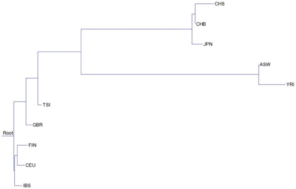
The inferred population tree from ten populations in the 1000 Genomes Project using 20 haplotypes from then individual per population. Branch length shown is the estimated time in coalescent units

6 Discussion and conclusions

In this article, we present the CompactCH algorithm for computing the gene tree probability under the multispecies coalescent model. While CompactCH is much faster than the STELLS when the number of populations is small, computing the exact gene tree probability for more populations remains a challenging task (Table 2). Nonetheless, we show in this article that efficient computation of gene tree probability for small number of (say two) populations can find applications in the inference of population history. We believe the CompactCH algorithm is a step forward for more efficient computation on coalescent models. The key idea of CompactCH is using compact coalescent histories. While merging multiple entities is a common idea in algorithm design, designing a working algorithm for coalescent computation based on this high-level idea is not trivial, as we show in this article. Our work suggests that coalescent computation can indeed be made more efficient by a well-designed algorithm [see Wu (2010) for an algorithm that speeds up coalescent computation under a different formulation].

We note that coalescent histories (in particular the mathematical properties of coalescent histories) have been actively studied recently [see e.g. Rosenberg 2013]. Our result presented here demonstrates that computation based on coalescent history can also be improved computationally. The CompactCH approach may also lead to speedup in coalescent computation in other formulations, where more complex coalescent models are used and computational efficiency is highly desirable. For example, the coalescent likelihood computed by MCMC in Heled and Drummond (2010) considers sequences, not the gene trees inferred from the sequences. Our techniques may be applied to speed up the computation of such likelihood.

References

- The 1000 Genomes Project Consortium (2015) A global reference for human genetic variation. Nature, 526, 64–74. [DOI] [PMC free article] [PubMed] [Google Scholar]
- Degnan J.H, Salter L.A. (2005) Gene tree distributions under the coalescent process. Evolution, 59, 24–37. [PubMed] [Google Scholar]
- Gusfield D. (1991) Efficient algorithms for inferring evolutionary history. Networks, 21, 19–28. [Google Scholar]
- Hein J., Schierup M., Wiuf C. (2005) Gene Genealogies, Variation and Evolution: A Primer in Coalescent Theory. Oxford University Press, UK. [Google Scholar]
- Heled J, Drummond A.J. (2010) Bayesian inference of species trees from multilocus data. Mol. Biol. Evol., 27, 570–580. [DOI] [PMC free article] [PubMed] [Google Scholar]
- Hudson R.R. (2002) Generating samples under the Wright-Fisher neutral model of genetic variation. Bioinformatics, 18, 337–338. [DOI] [PubMed] [Google Scholar]
- Hudson R.R. (1983) Testing the constant-rate neutral allele model with protein sequence data. Evolution, 37, 203–217. [DOI] [PubMed] [Google Scholar]
- Kimura M. (1969) The number of heterozygous nucleotide sites maintained in a finite population due to steady flux of mutations. Genetics, 61, 893–903. [DOI] [PMC free article] [PubMed] [Google Scholar]
- Kingman J.F.C. (1982) The coalescent. Stochast. Process. Appl., 13, 235–248. [Google Scholar]
- Mirarab S. et al. (2014) Astral: genome-scale coalescent-based species tree estimation. Bioinformatics, 30, i541–i548. [DOI] [PMC free article] [PubMed] [Google Scholar]
- Pickrell J.K, Pritchard J.K. (2012) Inference of population splits and mixtures from genome-wide allele frequency data. PLoS Genet., 8, e1002967.. [DOI] [PMC free article] [PubMed] [Google Scholar]
- Rosenberg N.A. (2002) The probability of topological concordance of gene trees and species trees. Theor. Popul. Biol., 61, 225–247. [DOI] [PubMed] [Google Scholar]
- Rosenberg N.A. (2013) Coalescent histories for caterpillar-like families. IEEE/ACM Trans. Comput. Biol. Bioinformatics, 10, 1253–1262. [DOI] [PubMed] [Google Scholar]
- Takahata N., Nei M. (1985) Gene genealogy and variance of interpopulational nucleotide differences. Genetics, 110, 325–344. [DOI] [PMC free article] [PubMed] [Google Scholar]
- Tavarè S. (1984) Line-of-descent and genealogical processes, and their applications in population genetics models. Theor. Popul. Biol, 26, 119–164., [DOI] [PubMed] [Google Scholar]
- Wakeley J. (2008) Coalescent Theory: An Introduction. Roberts and Company Publishers, Greenwood Village, CO, USA. [Google Scholar]
- Watterson G.A. (1984) Lines of descent and the coalescent. Theor. Popul. Biol., 26, 77–92. [Google Scholar]
- Wu Y. (2010) Exact computation of coalescent likelihood for panmictic and subdivided populations under the infinite sites model. IEEE/ACM Trans. Comput. Biol. Bioinformatics, 7, 611–618. [DOI] [PubMed] [Google Scholar]
- Wu Y. (2012) Coalescent-based species tree inference from gene tree topologies under incomplete lineage sorting by maximum likelihood. Evolution, 66, 763–775. [DOI] [PubMed] [Google Scholar]
- Wu Y. (2015) A coalescent-based method for population tree inference with haplotypes. Bioinformatics, 31, 691–698. [DOI] [PMC free article] [PubMed] [Google Scholar]
Associated Data
This section collects any data citations, data availability statements, or supplementary materials included in this article.