

Abstract
Motivation: Protein homology detection, a fundamental problem in computational biology, is an indispensable step toward predicting protein structures and understanding protein functions. Despite the advances in recent decades on sequence alignment, threading and alignment-free methods, protein homology detection remains a challenging open problem. Recently, network methods that try to find transitive paths in the protein structure space demonstrate the importance of incorporating network information of the structure space. Yet, current methods merge the sequence space and the structure space into a single space, and thus introduce inconsistency in combining different sources of information.
Method: We present a novel network-based protein homology detection method, CMsearch, based on cross-modal learning. Instead of exploring a single network built from the mixture of sequence and structure space information, CMsearch builds two separate networks to represent the sequence space and the structure space. It then learns sequence–structure correlation by simultaneously taking sequence information, structure information, sequence space information and structure space information into consideration.
Results: We tested CMsearch on two challenging tasks, protein homology detection and protein structure prediction, by querying all 8332 PDB40 proteins. Our results demonstrate that CMsearch is insensitive to the similarity metrics used to define the sequence and the structure spaces. By using HMM–HMM alignment as the sequence similarity metric, CMsearch clearly outperforms state-of-the-art homology detection methods and the CASP-winning template-based protein structure prediction methods.
Availability and implementation: Our program is freely available for download from http://sfb.kaust.edu.sa/Pages/Software.aspx.
Contact: xin.gao@kaust.edu.sa
Supplementary information: Supplementary data are available at Bioinformatics online.
1 Introduction
Protein homology detection, that aims to identify protein homologs that share a common ancestry during the course of evolution, is one of the fundamental open problems in computational biology. For close homologs, sequence similarity search tends to be sufficient (Arnold et al., 2006). However, instead of sharing similar sequences, remote homologs might only share similar tertiary (3D) structures or similar functions. This is because protein structures and functions are more conserved than sequences due to the evolutionary pressure (Marks et al., 2012; Messih et al., 2012). Because of the high cost and experimental barriers to determine protein structures and functions, biologists frequently stuck in the situation that only the sequence is available for the protein of interest. Thus, computationally detecting remote homologs from a database of proteins with known sequences and/or structures becomes a challenging and essential problem (Ben-Hur and Brutlag, 2003).
Generally, existing methods for protein homology detection can be divided into three categories: alignment-free methods, alignment methods and network methods. The alignment-free methods refer to the approaches that represent a protein as a feature vector and then search for homologs in the protein database by comparing feature vectors. Early methods, such as Park et al. (1998), conduct direct comparisons of feature vectors. Later discriminative methods, such as Liu et al. (2014) which is based on support vector machines, have been developed to improve the sensitivity. However, a recent study indicates that the alignment-free methods are usually faster but less sensitive compared to alignment methods (Ma et al., 2014).
The alignment methods refer to the approaches that search the query protein against proteins in the database through alignments. These methods can either rely on sequences only or employ structure features as well, where the latter is also called threading (Cheng and Baldi, 2006; Jo et al., 2015; Karplus et al., 1998; Wang et al., 2012a,b; Wu and Zhang, 2008). The most successful methods that rely on sequences only include the ones that enrich protein sequence information by position-specific scoring matrices (PSSMs) (Altschul et al., 1997), hidden Markov models (HMMs) (Finn et al., 2011) or Markov random fields (MRFs) (Daniels et al., 2012; Ma et al., 2014). For threading methods, in addition to the enriched sequence information, the structure features—such as secondary structures (Jones, 1999), solvent accessibility (Lee and Richards, 1971) and residue-residue contacts (Cheng and Baldi, 2007; Gao et al., 2009)—predicted from the query protein sequence, are compared to the structure features extracted from the 3D structures in the database.
Neither alignment-free nor alignment methods exploit the network topologies of the protein space because they predict homologs in a pairwise comparison manner (i.e. either one-to-one or one-to-family) (Melvin et al., 2011). This motivates network methods to connect remote homologs through a transitive path in the continuous protein space (Nepomnyachiy et al., 2014). Early network methods utilize sequence similarities to construct the protein network, but they show minor improvement over the sequence alignment methods (Melvin et al., 2011). Recently, ENTS (Enrichment of Network Topological Similarity) was proposed (Lhota et al., 2015) which constructs a structure similarity network for proteins in the Protein Data Bank (PDB) and then links the query protein sequence to the known structures through sequence similarities. Although ENTS has demonstrated its outstanding performance, it should be considered as a structure similarity-based network method except for the query protein. Specifically, when building the protein network, only structure similarities are used for the proteins in the database, and the sequence similarity is only used to approximate the structure similarity for the query protein. Thus, ENTS used sequence and structure similarities in a mixed manner, but it is known that there is no standard way to combine different similarity metrics in a unified fashion. As demonstrated later in Section 3.1, this might introduce inconsistency issues.
In this article, we propose a cross-modal method, CMsearch, for protein homology detection. As shown in Figure 1, CMsearch employs not only structure similarities but also sequence similarities. It then explores the structure and the sequence spaces (networks) simultaneously by learning sequence–structure correlations (cross-modal links) between the structure and the sequence spaces. To our knowledge, CMsearch is the first method that is able to incorporate sequence information, structure information, sequence space information and structure space information simultaneously. Specifically, as shown in Table 1, CMsearch has several advantages over existing methods: (i) Instead of exploring a single space built from the mixture of sequence and structure similarities as ENTS (Lhota et al., 2015), CMsearch builds two separate spaces and explores the two spaces simultaneously. (ii) CMsearch is completely different from threading methods because it uses not only sequence and structure information, but also sequence and structure space information. (iii) CMsearch is a generic framework such that any sequence similarity metric and any structure similarity metric can be adopted.
Fig. 1.

Illustration of CMsearch: each yellow box represents a protein structure; each green line represents a protein sequence; each blue arrow represents a cross-modal link. CMsearch incorporates sequence information, structure information, sequence network topologies in the sequence space and structure network topologies in the structure space simultaneously and directly learns the structure–sequence correlations (i.e. cross-modal links)
Table 1.
Input data used by homology detection methods: SEQ refers to any kind of sequence features extracted from the query sequence, such as a multiple sequence alignment represented by a PSSM, an HMM, or an MRF; STR refers to any kind of structure features predicted from the query sequence or extracted from the target structures, such as secondary structures, solvent accessibilities, and residue-residue contacts; SEQ NET refers to the network topologies in the protein sequence space; and STR NET refers to the network topologies in the protein structure space
| Method | Input data | |||
|---|---|---|---|---|
| SEQ | STR | SEQ NET | STR NET | |
| Sequence alignment | ✓ | × | × | × |
| Threading | ✓ | ✓ | × | × |
| ENTS | ✓ | ✓ | × | ✓ |
| CMsearch | ✓ | ✓ | ✓ | ✓ |
We test the performance of CMsearch on two very challenging tasks, protein homology detection and protein structure prediction, by querying all 8332 proteins in the PDB40 dataset. Our results demonstrate that CMsearch is insensitive to the similarity metric. It can significantly improve the homology detection performance to the similar levels no matter which sequence similarity metric is used to define the sequence space. By using HMM–HMM alignment as the sequence similarity metric, CMsearch clearly outperforms state-of-the-art homology detection methods, including HHsearch (Söding, 2005), RaptorX (Ma et al., 2012) and ENTS (Lhota et al., 2015). When CMsearch is applied to structure prediction of PDB40, it outperforms CASP-winning template-based structure prediction methods. For hundreds of cases, it can predict highly accurate models (TM-score above 0.6) while the existing methods cannot.
2 Methods
2.1. Problem formulation
CMsearch incorporates sequence information, structure information, sequence network topologies in the sequence space and structure network topologies in the structure space simultaneously and directly learns the structure–sequence correlations (as illustrated in Fig. 1). Specifically, the protein sequence space is defined as a sequence similarity network, in which each node is a protein sequence and two sequences have an edge if their pairwise sequence similarity is higher than a threshold by a certain similarity metric, where the edge weight is the similarity value. Here, the protein sequence space is denoted as , where si is the i-th sequence, and n is the number of sequences in this space. Protein structure space is defined in a similar way, as a structure similarity network, by using a certain structure similarity metric. Here, the protein structure space is denoted as , where tj is the j-th structure, and m is the number of the structures in this space. The terms, space and similarity network, will be used interchangeably throughout the article.
The problem of cross-modal search is to learn the correlations between the protein sequences in and the protein structures in , and the sequence–structure pairs with strong correlations are predicted to be homologs. Here, the cross-modal link correlation matrix is denoted as , where its (i, j)-th element is the degree of correlation between si and tj. With matrix X, we can obtain the cross-modal links, , as the high correlation values in X. Moreover, we have an initial cross-modal link set as the input of this problem, which is denoted as . Specifically, if a sequence–structure pair, (si, tj), is obtained from the same protein, it is included in . More detailed data collection procedures are provide in Section 2.3. This initial link set is sparse, but it could be a sufficient starting point to learn the complete and accurate link set, . To present the initial link set, we also define an initial correlation matrix, , where
| (1) |
This way, the problem of cross-modal search is transferred to the problem of learning X from and . To learn an optimal X, we utilize the existing link information contained in , the sequence similarity information of sequences in , and the structure similarity information of structures in . To this end, we consider the following objectives to construct the loss function:
Respecting initial links: To utilize the initial information represented by , we impose the learned matrix X to be close to , so that the learned X can respect the initial links. We use the squared -norm distance to measure how close X is to , and minimize it to construct the first loss term,
| (2) |
Sequence similarity regularization: To present the sequence information of , we construct a neighborhood graph from . The graph is denoted as , where is the set of nodes of the graph, and each node represents a sequence. is the set of edges of the graph, and it is defined between each sequence and its neighbors, , where is the set of the nearest neighbors of si according to a given sequence similarity which will be discussed later, is the sequence similarity between si and sj, and is a sequence similarity threshold for highly-confident homologs. The goal of this process is to make sure that most of the connected neighbors are protein homologs so that it is safe to learn the complete network from the initial incomplete network. is a corresponding symmetric similarity matrix, and its (i, j)-th element is the similarity between si and sj,
| (3) |
Note that the i-th row of X (denoted as ) is the confidence of si being linked to the m structures of . If sequences si and sj are similar to each other, i.e., γij is large, we expect that and are close to each other as well. We measure how close and are to each other by a squared -norm distance, and minimize this distance between each pair of weighted by normalized γij,
 |
(4) |
where Tr is the trace function of a matrix, is the normalized graph Laplacian (Doyle and Snell, 1984) of the sequence space, and is a diagonal matrix with its (i, i)-th element . Thus, if a pair of sequences (si, sj) are similar to each other, their corresponding rows and are also imposed to be close to each other.
Structure similarity regularization: To incorporate the structure space information, we construct a neighborhood graph from in a similar way, and its corresponding normalized similarity matrix is denoted as , where
| (5) |
where is the set of the nearest neighbors of ti according to a structure similarity metric, is the structure similarity between ti and tj, and is a structure similarity threshold for highly confident protein homologs. The i-th column of X is the confidence of ti being linked to the sequences in (denoted as ). If two structures, ti and tj, are similar to each other, i.e., δij is large, we expect that and are close to each other. Thus we propose to minimize the following objective,
 |
(6) |
where is the normalized graph Laplacian of the structure space, and is a diagonal matrix with its (i, i)-th element .
The final optimization problem is thus a combination of the objectives in (2), (4) and (6),
| (7) |
where and are trade-off parameters. By solving this problem, we can obtain X, which simultaneously respects the initial , the sequence space , and the structure space .
2.2. Problem optimization
To solve the problem in (7), we can directly set its derivative with respect to X to zero,
| (8) |
This is a Sylvester matrix equation, and it has a unique solution because both and are positive definite (Bartels and Stewart, 1972). However, solving this equation is very time-consuming, and we thus adopt an alternate method to optimize (7) by using an approximate two-step strategy (Lu and Peng, 2013; Zhou et al., 2004). The objective function is split into two parts:
| (9) |
where is the objective of X regularized only by the sequence similarity, while is that regularized only by the structure similarity. In the first step, we minimize with regard to X, to obtain a solution . In the second step, we use as the initial link confidence matrix to replace in , and minimize with regard to X to obtain the final solution. The details are as follows:
Step I: We solve the following problem to obtain the intermediate optimal solution ,
| (10) |
It has been shown that this optimization problem can be solved by an iterative label propagation method (Zhou et al., 2004). Specifically, in each iteration, the current link confidence matrix Xcur is updated from the previous link confidence matrix Xpre,
| (11) |
where is the normalized sequence similarity matrix, and is a weighting parameter derived from . The label propagation iterations above have been proved to converge (Zhou et al., 2004) to,
| (12) |
Step II: We replace in by , and solve the following problem to obtain the final link confidence matrix ,
| (13) |
Similarly, this optimization problem can be solved by an iterative label propagation method,
| (14) |
where is the normalized structure similarity matrix, and is a weighting parameter derived from . Finally, the above label propagation iterations converge to,
| (15) |
Substituting the solution in (12) to (15), we have the final optimization result of ,
| (16) |
2.3. Dataset
In order to comprehensively evaluate the performance of CMsearch, we carefully selected a dataset, referred as the PDB40, which consists of 10 288 proteins from the PDB. We downloaded the CULLPDB subset (Wang and Dunbrack, 2003) of PDB with a sequence identity cutoff of 40%, an X-ray crystallography resolution cutoff of 2.0 Å, and an X-ray crystallography R-factor cutoff of 0.25 on March 14, 2015. Proteins with less than 50 residues or more than 1000 residues, and proteins formed only by a small number of α-helices were removed. This yielded a complete, non-redundant and high-quality protein dataset representing all proteins in PDB.
To build the structure similarity matrix Δ for PDB40, we calculated the TM-score (Zhang and Skolnick, 2004) for each pair of proteins within PDB40 and used the pairwise TM-score matrix as Δ. Here, TM-score was selected because it is the most widely used and acknowledged similarity metric for protein structure comparison and it has two important properties: (i) TM-score is independent from the number of residues of proteins; and (ii) TM-score has a range between zero and one, and a TM-score higher than 0.5 suggests that the two aligned protein structures tend to be within the same protein fold whereas a TM-score above 0.6 suggests highly similar structures (Xu and Zhang, 2010). Note that any other structure alignment and similarity metric can be used instead of TM-score (Cui et al., 2013, 2015a,b), but finding the optimal structure similarity metric is out of the scope of this study.
To build the sequence similarity matrix Γ, we used three different popular sequence similarity metrics separately (instead of combining them together). The first metric is the e-value of sequence-HMM alignment calculated by HMMER (Finn et al., 2011), the second one is the homologous probability of HMM–HMM alignment calculated by HHsearch (Söding, 2005) and the third one is the MRF–MRF alignment score calculated by MRFalign (Ma et al., 2014). Specifically, for each pair of proteins (i, j), we set for the e-value E(i, j) calculated by HMMER, for the homologous probability P(i, j) calculated by HHsearch, and for the alignment score S(i, j) calculated by MRFalign. Consequently, all sequence similarities have a range between zero and one. Again, any other sequence similarity metric can be used here.
Finally, we set the initial cross-modal correlation matrix according to the one-to-one mapping between and . Specifically, for a sequence i in and a structure j in , we set if they are from the same protein. Otherwise, . Note that it is also possible to initialize by incorporating highly confident sequence–structure pairs found by existing threading methods, which is currently under investigation.
Given the sequence similarity matrix Γ, the structure similarity matrix Δ, and the initial cross-modal link matrix , CMsearch learns all cross-modal links between the sequence space and the structure space. This includes the cross-modal links between the query protein sequences in the sequence space (without known structures) and their homologs in the structure space.
3 Results and discussion
3.1. Performance on 32-fold cross-validation homology detection
3.1.1. Experimental procedure
We performed a 32-fold cross-validation (CV) on PDB40 for each homology detection method compared in this article. First, the PDB40 dataset was randomly divided into 32 disjoint subsets, and the homology detection process was repeated 32 times. For each time, one subset was used as the query proteins (only sequences were known), and the remaining ones were used as the database (with both known sequences and structures) from which each method tries to identify homologs to the queries. For all methods, the structures of the query proteins were not used as inputs. For CMsearch, this was done by removing the rows and the columns corresponding to the query proteins from the structure similarity matrix Δ and the initial cross-modal matrix .
In this experiment, protein homologs are defined as structurally similar proteins with TM-scores (Zhang and Skolnick, 2004) above 0.6. Such a TM-score threshold guarantees that the protein homologs share the same SCOP (Structural Classification of Proteins) fold and are high-quality structure templates to build 3D structures (Xu and Zhang, 2010). Actually, other TM-score thresholds between 0.4 and 0.6 have also been tested, and similar conclusions can be drawn no matter which threshold is used. Thus, due to the page limit, we focus on the high-confidence threshold of 0.6 in this article. Using this definition, if a query protein does not have any homolog in the database, it is not included in the analysis. As a result, 8332 proteins from the PDB40 dataset were selected for the analysis.
To evaluate the performance of different homology detection methods, we used three widely used performance measures: precision, recall and area under the precision-recall curve (AUPRC). For each query protein in one of the 32 folds, each method was used to find (i.e. to predict) all protein homologs from the remaining 31 folds, and a confidence score was calculated by this method for each predicted homolog. Precision and recall for the top K predictions for each method were calculated, where K was set to 1, 3, 5, 10, 25, 50 and 100. Precision is defined as the number of true homologs among the top K predictions over K, and recall is defined as the number of true homologs among the top K predictions over the total number of homologs of this query. The AUPRC is an overall summary of the precision–recall curve which is well suited for the homology detection task because the number of non-homologs is significantly larger than that of homologs, which will cause the area under the receiver operating characteristic curve to present an overly optimistic view (Davis and Goadrich, 2006).
3.1.2. Results and discussion
First, we demonstrate that, given any state-of-the-art sequence similarity metric, CMsearch with the protein sequence space defined by this similarity metric always outperforms homology detection using this sequence similarity alone. To this end, we tested CMsearch on three state-of-the-art sequence similarity metrics, sequence–HMM alignment by HMMER (Finn et al., 2011), HMM–HMM alignment by HHsearch (Söding, 2005) and MRF–MRF alignment by MRFalign (Ma et al., 2014). For each of these methods, it was first used to score the similarity between a query protein and the sequences in the corresponding database of the 32-fold CV, and the top-scored K proteins were used as the predictions of homologs for this method. The same method was then used to define the sequence space which was used as the input to CMsearch. CMsearch then combined sequence space defined by this method and structure space defined by TM-score to learn the correlation between the query protein and the proteins in the database, and returned the top-scored K proteins as the predictions of homologs. Note that no consensus approach was taken in any step. The three sequence similarity metrics were tried one by one, separately.
As shown in Figure 2, in all three cases of sequence similarity metrics, CMsearch is able to significantly improve both recall and precision of the corresponding method regardless of the value of K. Among the three original methods, MRFalign (Ma et al., 2014) tends to be the best method and HHsearch (Söding, 2005) is a close second. However, after incorporating the sequence space information and structure space information, the three versions of CMsearch tend to have similar performance as the precision curves and the recall curves stay close to each other. In terms of AUPRC, CMsearch improves the AUPRC of HMMER, HHsearch and MRFalign from 0.74, 0.76 and 0.78 to 0.86, 0.87 and 0.89, respectively, which demonstrates a relative improvement of at least 14%. Therefore, CMsearch can substantially improve the homology detection performance regardless of the input sequence similarity metrics.
Fig. 2.

Precision and recall of homology detection when different numbers of top predictions are considered by three sequence similarity metrics versus CMsearch (using the corresponding metric for the sequence space): dashed lines denote the original sequence similarity methods; solid ones denote the corresponding versions of CMsearch; and the AUPRC for HMMER, HHsearch and MRFalign is 0.74, 0.76 and 0.78, whereas that for the corresponding versions of CMsearch is 0.86, 0.87 and 0.89, respectively
Next, we compare CMsearch with CASP-winning protein homology detection methods, including HHsearch (Söding, 2005), RaptorX (Källberg et al., 2012; Ma et al., 2012) and ENTS (Lhota et al., 2015). We hereinafter fix the sequence similarity metric in CMsearch to be HHsearch because of its excellent balance between accuracy and speed, and remain using TM-score as the structure similarity metric. As shown in Figure 3, recall always increases for different methods when K increases. This is expected because the number of true homologs does not change when K increases. Thus, including more predicted homologs (i.e. a bigger K) will cover more true homologs. Similarly, the precision should be expected to decrease when K increases because including more predicted homologs will more likely cover false homologs. However, such a reasoning does not necessarily hold, as shown for ENTS when K is smaller than 10. In general, HHsearch and RaptorX have quite similar precision, while HHsearch is slightly more sensitive than RaptorX. Under all settings of K, CMsearch is always the method with the highest precision and recall.
Fig. 3.
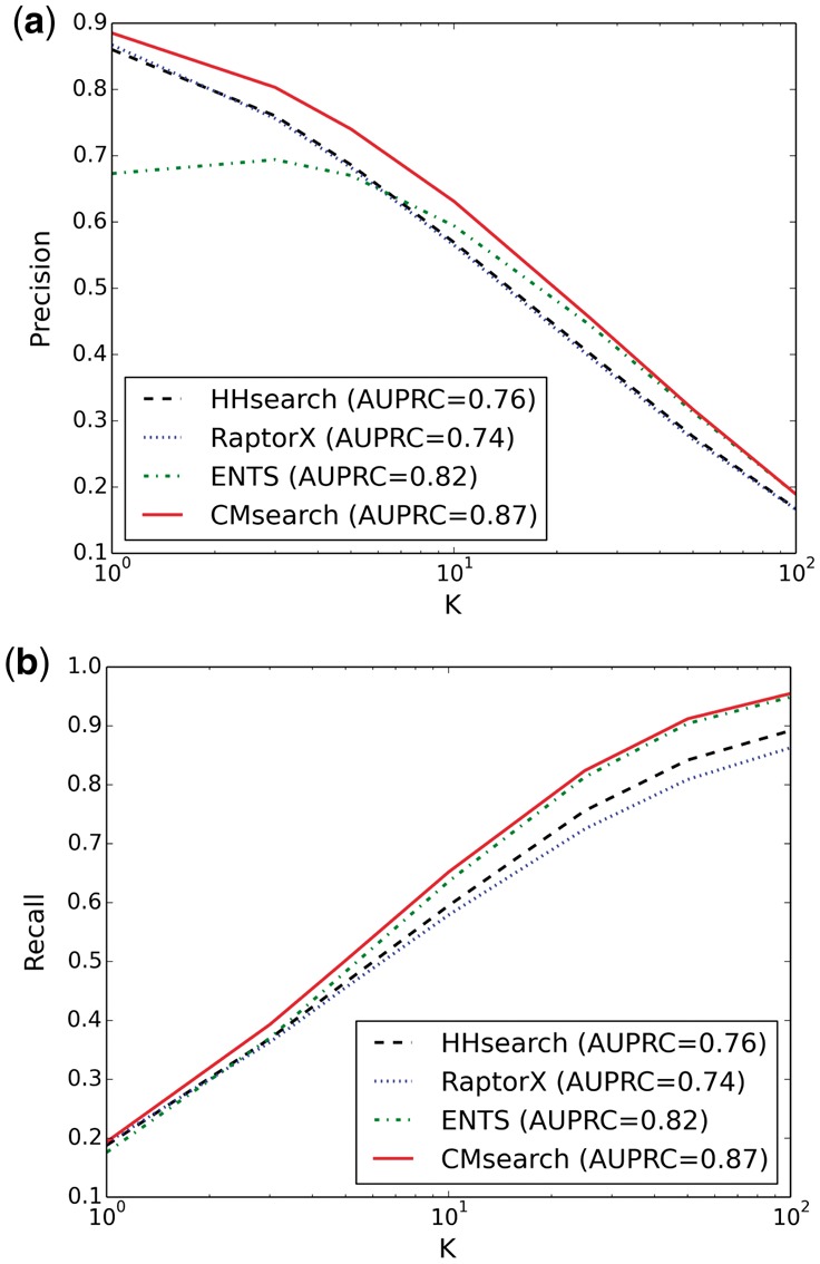
Precision and recall of homology detection when different numbers of top predictions are considered by HHsearch, RaptorX, ENTS and CMsearch (with HHsearch as the sequence similarity metric): for K = 10, the precision for the four methods is 0.57, 0.57, 0.59 and 0.63, respectively, and the recall for the four methods is 0.60, 0.58, 0.64 and 0.65, respectively
According to the Continuous Automated Model EvaluatiOn of predicted 3D protein structures (CAMEO-3D) (Haas et al., 2013), RaptorX (Ma et al., 2012; Källberg et al., 2012) is the most accurate protein structure prediction method based on the results of the second half of year 2015. Actually, finding protein homologs as structure templates is critical to the success of the template-based RaptorX method. Comparing RaptorX and CMsearch in Figure 3, CMsearch achieves significantly higher precision, recall and AUPRC than RaptorX regardless of K. For example, when K = 10, RaptorX achieves a solid performance with a precision of 0.57, a recall of 0.58 and an AUPRC of 0.74, whereas CMsearch obtains a precision of 0.63, a recall of 0.65 and an AUPRC of 0.87. This reflects a 11–18% improvement over RaptorX. Our results demonstrate that simultaneously combining sequence space information and structure space information can significantly boost the accuracy of protein homology detection, and thus potentially improve the accuracy of template-based protein structure prediction (more evidences shown in Section 3.2).
ENTS (Lhota et al., 2015) is also a network-based method that tries to perform learning on a single space that is defined by the mixture of both structure similarities and sequence similarities. However, the heterogeneity of the two types of similarities caused inconsistency in the network. This can be demonstrated as the promising performance of ENTS when K is big, but a surprisingly low precision when K is small. This suggests that performing cross-modal learning between the two separately defined networks is more reliable than learning in an arbitrarily combined network. Similar conclusions can be drawn when we repeated the homology detection experiments on PDB30 (Supplementary Fig. S1).
3.2. Performance on PDB-wide structure prediction
3.2.1. Experimental procedure
We then tested the performance of protein structure prediction based on the predicted homologs from the previous experiment over the entire PDB40 dataset, using the same 32-fold CV. Note that all 8332 proteins were used as queries exactly once. To our knowledge, this is by far the largest query set used to benchmark protein structure prediction methods.
For each pair of a query protein sequence and a predicted homolog by a method (with a known structure), multiple pairwise alignments were generated by calling existing alignment methods: HMMER (Finn et al., 2011), HHalign (Söding, 2005) MRFalign (Ma et al., 2014) and RaptorX (Ma et al., 2012). For each generated alignment, the protein homolog was used as a structure template, and a structure of the query protein was generated by calling Modeller (Eswar et al., 2006) which is the most widely used model generation method with proven success (Hildebrand et al., 2009; Källberg et al., 2012; Roy et al., 2010). For each query protein, the best predicted model among all predicted structure models was selected as the one with the highest TM-score to the native structure.
Given the best predicted model among the top 10 predictions by a method and the native structure of each query protein, we used several widely-used structure evaluation metrics to measure the quality of the predicted model, including TM-score (Zhang and Skolnick, 2004), GDT-HA score (Zemla, 2003), and root-mean-square deviation (RMSD). For each evaluation metric, an average score of all query proteins over all 32-fold CV was calculated as the final result of a method. Here we report the comparison between the best models among the first 10 returned models by HHsearch (Söding, 2005), RaptorX (Källberg et al., 2012), ENTS (Lhota et al., 2015) and CMsearch by using HHsearch as the sequence similarity metric.
3.2.2. Results and discussion
The qualities of the protein structures predicted by different methods are compared in Figure 4. The black points are the easy cases where both methods can produce high-quality models (TM-score above 0.6). The red and the blue points are interesting cases, such that one of the two methods fails to predict high-quality models, but the other method manages to ‘rescue’ the query proteins by predicting high-quality models. Among these interesting cases (also reported in Table 2), it can be seen that CMsearch has a remarkable advantage over all the other methods. For example, CMsearch is able to rescue 13, 2 and 11 times more query proteins than HHsearch, RaptorX and ENTS, respectively, while the average TM-score of CMsearch over the red and blue points improves that of the competing methods by 31%, 14% and 16%. Since all methods compared here call Modeller to build structure models, the only possible reason for the performance improvement is because of better homologs detected by CMsearch.
Fig. 4.

TM-scores of the predicted structure models by using the homologs (i.e. structure templates) found by HHsearch, RaptorX and ENTS versus using those found by CMsearch: the black points represent the cases where both methods can predict high-quality structures (with TM-scores above 0.6), which should be considered as the easy cases; the gray points represent the opposite cases where both methods cannot predict high-quality models; the red points represent the cases where the competing method cannot predict any high-quality models but CMsearch can; and the blue points represent the opposite cases where CMsearch cannot predict any high-quality models while the competing method can (statistics related to these figures are shown in Table 2)
Table 2.
Comparison of the predicted structure models by using the homologs (i.e. structure templates) found by HHsearch, RaptorX and ENTS versus using those found by CMsearch
| Methods | All regions | Red and blue regions | |||||||||
|---|---|---|---|---|---|---|---|---|---|---|---|
| TM-score | GDT-HA | RMSD(Å) | Count | TM-score | |||||||
| Mean | Std | Mean | Std | Mean | Std | Nred | Nblue | Mean | CMsearch | Imprv (%) | |
| HHsearch | 0.743 | 0.160 | 0.481 | 0.149 | 4.27 | 0.92 | 505 | 40 | 0.515 | 0.675 | 31.1 |
| RaptorX | 0.770 | 0.142 | 0.495 | 0.143 | 5.31 | 1.58 | 203 | 102 | 0.547 | 0.625 | 14.3 |
| ENTS | 0.744 | 0.160 | 0.480 | 0.147 | 4.17 | 0.94 | 401 | 37 | 0.549 | 0.639 | 16.4 |
| CMsearch | 0.774 | 0.139 | 0.500 | 0.142 | 4.14 | 0.98 | − | − | − | − | − |
Note: For all 8332 query proteins of the PDB40 dataset, the averages and the standard deviations of TM-score, GDT score and RMSD are reported; for the red and the blue points in Figure 4, CMsearch is able to increase the number of high-quality models by a factor of 12.6 (505 versus 40) and improve the average TM-score by 31.1% (0.675 versus 0.515) over HHsearch. The best performance under each performance measure is in bold.
The overall structure prediction accuracy is reported in Table 2. CMsearch always has the best performance no matter which evaluation criterion is used, while RaptorX is the second best one. Considering that protein structure prediction has been a well-studied yet challenging problem for more than seven decades, it is highly unlikely to significantly improve the easy cases that form the majority of the dataset. Consequently, significant improvement on hard cases might be averaged out when evaluating the average performance. Meanwhile, our benchmark dataset is much larger and comprehensive than any previous study, which makes improving the average performance even more challenging. Despite such difficulties, the Wilcoxon test on the paired TM-scores over the 8332 query proteins shows that the improvement of CMsearch over the three methods is significant. Specifically, the P-value for the paired TM-scores between RaptorX (0.770) and CMsearch (0.774) is 9.17E-87, whereas those between CMsearch and the other two methods are even much lower.
3.3. Case studies
Here we describe three representative examples of our results. The first one is PDB id 2ODA chain A (hereinafter called 2ODAA), a protein from the plant pathogen Pseudomonas syringae (Peisach et al., 2008). It is a representative member of a subfamily of the haloacid dehalogenase superfamily. All the top 10 ranked predicted models by CMsearch have TM-score of 0.6 or above, with TM-score of the top model being 0.686 (Fig. 5d). The template selected by CMsearch for this model is alnumycin B (PDB id 4EX6A), which is an enzyme of the same haloacid dehalogenase superfamily as 2ODAA. In contrast, for HHsearch, ENTS and RaptorX, all of their top 10 ranked predicted models have TM-score below 0.6. The first models predicted by the three methods are shown in Figure 5(a–c), with TM-score of 0.548, 0.132 and 0.519, respectively.
Fig. 5.

Superpositions of the best template model (cyan) to the native model (magenta): the best template model is found by HHsearch, RaptorX, ENTS or CMsearch for query protein: (a–d) 2ODAA, (e–g) 3VCXA or (h–i) 2Q73A (note that the same template model might be found by different methods); and the models are superimposed by TM-align and the superimposed models are visualized by PyMOL
The second example is 3VCXA, a putative glyoxalase/bleomycin resistance protein from Rhodopseudomonas palustris. Among the top 10 ranked models of HHsearch, ENTS, RaptorX and CMsearch, 4, 3, 5 and 8 of them have TM-score of 0.6 or above, respectively. The top model of CMsearch has TM-score of 0.761 (Fig. 5g), which is dramatically more accurate than that of the three other methods (with TM-score of the top model being 0.385, 0.380 and 0.380, respectively) (Fig. 5(e–f)). 3VCXA has known Gene Ontology annotations. It is involved in dioxygenase activity as molecular function (MF) and oxidation reduction process as biological process (BP). Both HHsearch and ENTS select 3R6AA as the top template, which has lactoylglutathione lyase activity and lyase activity as MF, and metabolic process as BP. RaptorX selects 3OXHA as the top template, which has unknown MF or BP annotation. CMsearch, on the other hand, selects 4HC5A as the top template, which has exactly the same function annotation as 3VCXA, and is also a glyoxalase/bleomycin resistance protein, but from Sphaerobacter thermophilus.
The third example is 2Q73A, which is a MazG nucleotide pyrophosphohydrolase domain (Robinson et al., 2007). Among the top 10 models of the four methods, HHsearch, ENTS and RaptorX each has one model of TM-score above 0.6, whereas CMsearch has two. Interestingly, although HHsearch, ENTS and RaptorX all select 4QGPA as the template for the top model (Fig. 5h), CMsearch selects 1VMGA as the top template (Fig. 5i), both of which are also MazG nucleotide pyrophosphohydrolase domains. However, 1VMGA tends to be a better template because the TM-score of the final model is 0.747, whereas that for 4QGPA is 0.536. It is worth noting that there are only two templates in the entire PDB40 that have TM-score of above 0.6 to the native structure of 2Q73A, and CMsearch returns them as the first and third ranked templates.
We further look into the reason why CMsearch is able to detect better homologs and rank them at the top for the three cases. It turns out that HHsearch, for instance, can detect strong query-sequence links in the sequence space (solid blue lines in the sequence space in Fig. 6), follow which it can identify the corresponding sequence–structure pairs (solid blue lines between the two spaces). Thus, each prediction of HHsearch is equivalent to finding a path from the query, through a sequence in the sequence space, to the corresponding structure in the structure space. However, in these cases, the top homologs selected by HHsearch are ‘inconsistent’. Taking 2ODAA, for example, the pairwise sequence links (in the sequence space) among the top three homologs by HHsearch are strong, weak and weak (relatively), whereas the corresponding pairwise structure links (in the structure space) are strong, strong and weak. Thus, the top three homologs by HHsearch do not well support each other because the true homologs of the query protein tend to be similar to each other (i.e. strong pairwise links in both the sequence and the structure spaces). In contrast, CMsearch simultaneously considers the weak query-sequence links (dashed red lines in the sequence space), the strong pairwise sequence links (solid red lines in the sequence space), the strong corresponding sequence–structure links (solid red lines between the two spaces) and the strong pairwise structure links (solid red lines in the structure space). This strong consistency compensates for the relatively weak query-sequence links, and hence CMsearch ranked these homologs at the top. Note that keeping consistency does not mean losing diversity of the selected homologs, but it penalizes cases such as strong sequence links with weak structure links, or violations of triangle inequality in the structure space.
Fig. 6.

Illustration of why CMsearch is able to detect better homologs and rank them at the top for the three cases in Figure 5: each triangle represents a sequence; each pentagon represents the corresponding structure; each solid line represents a strong link; each dashed line represents a (relatively) weak link; the top three homologs predicted by HHsearch (in blue) have strong query-sequence links; the top three homologs predicted by CMsearch (in red) have weak query-sequence links but strong links among the sequences and structures of them three; and this demonstrates that CMsearch is capable of compensating weak links to true homologs that are consistent (i.e. the true homologs tend to be similar to each other)
4 Conclusion
In this article, we proposed a cross-modal search method, CMsearch, for protein homology detection. CMsearch is capable of significantly improving the accuracy of state-of-the-art homology detection methods, including HMMER (Finn et al., 2011), HHsearch (Söding, 2005), MRFalign (Ma et al., 2014), RaptorX (Ma et al., 2012) and ENTS (Lhota et al., 2015). This demonstrates that combining sequence space information and structure space information can significantly boost the accuracy of protein homology detection and improve the accuracy of template-based protein structure prediction. The success of our method is mainly credited to the cross-modal propagation that simultaneously explores the protein sequence space and the protein structure space. The only cost of applying our method is approximately 10 min of computational time on an average computer.
Furthermore, our framework is generic and can be straightforward extended to multiple modals. It thus can be a highly valuable framework for many computational biology tasks. For example, we are currently extending our method to predict protein functions by simultaneously incorporating protein sequence space information, structure space information and gene ontology space information. It would also be interesting to investigate the possibility to use the network topologies in the sequence and the structure spaces to detect the number of homologs, or if there exists a homolog in the database or not. This information could be useful for protein structure prediction with multiple templates.
Supplementary Material
Acknowledgements
We thank Dr. Jinbo Xu for fruitful discussions and valuable comments.
Funding
The research reported in this publication was supported by the King Abdullah University of Science and Technology (KAUST) Office of Sponsored Research (OSR) under Award No. URF/1/1976-04, National Natural Science Foundation of China (61573363), the Fundamental Research Funds for the Central Universities and the Research Funds of Renmin University of China (15XNLQ01), and IBM Global SUR Award Program. This research made use of the resources of the computer clusters at KAUST.
Conflict of Interest: none declared.
References
- Altschul S.F. et al. (1997) Gapped BLAST and PSI-BLAST: a new generation of protein database search programs. Nucleic Acids Res., 25, 3389–3402. [DOI] [PMC free article] [PubMed] [Google Scholar]
- Arnold K. et al. (2006) The SWISS-MODEL workspace: a web-based environment for protein structure homology modelling. Bioinformatics, 22, 195–201. [DOI] [PubMed] [Google Scholar]
- Bartels R.H., Stewart G. (1972) Solution of the matrix equation AX+ XB= C [F4]. Commun. ACM, 15, 820–826. [Google Scholar]
- Ben-Hur A., Brutlag D. (2003) Remote homology detection: a motif based approach. Bioinformatics, 19 (Suppl 1), i26–i33. [DOI] [PubMed] [Google Scholar]
- Cheng J., Baldi P. (2006) A machine learning information retrieval approach to protein fold recognition. Bioinformatics, 22, 1456–1463. [DOI] [PubMed] [Google Scholar]
- Cheng J., Baldi P. (2007) Improved residue contact prediction using support vector machines and a large feature set. BMC Bioinform., 8, 113. [DOI] [PMC free article] [PubMed] [Google Scholar]
- Cui X. et al. (2013) Towards reliable automatic protein structure alignment. In: Proceedings of the 13th International Workshop, WABI 2013, pp. 18–32. Springer, Sophia Antipolis, France.
- Cui X. et al. (2015a). Compare local pocket and global protein structure models by small structure patterns. In: Proceedings of the 6th ACM Conference on Bioinformatics, Computational Biology and Health Informatics, BCB ’15, pp. 355–365. ACM, New York, NY, USA.
- Cui X. et al. (2015b) Finding optimal interaction interface alignments between biological complexes. Bioinformatics, 31, i133–i141. [DOI] [PMC free article] [PubMed] [Google Scholar]
- Daniels N.M. et al. (2012) SMURFLite: combining simplified Markov random fields with simulated evolution improves remote homology detection for beta-structural proteins into the twilight zone. Bioinformatics, 28, 1216–1222. [DOI] [PMC free article] [PubMed] [Google Scholar]
- Davis J, Goadrich M. (2006). The relationship between Precision-Recall and ROC curves. In: Proceedings of the 23rd International Conference on Machine Learning, University of Michigan, Mathematical Association of America. pp. 233–240. ACM.
- Doyle P.G., Snell J.L. (1984) Random walks and electric networks. AMC, 10, 12. [Google Scholar]
- Eswar N. et al. (2006) Comparative protein structure modeling using Modeller. Curr. Protoc. Bioinform., 39, W29–W37. [DOI] [PMC free article] [PubMed] [Google Scholar]
- Finn R.D. et al. (2011) HMMER web server: interactive sequence similarity searching. Nucleic Acids Res., gkr367.. [DOI] [PMC free article] [PubMed] [Google Scholar]
- Gao X. et al. (2009) Improving consensus contact prediction via server correlation reduction. BMC Struct. Biol., 9, 28. [DOI] [PMC free article] [PubMed] [Google Scholar]
- Haas J. et al. (2013) The Protein Model Portal - a comprehensive resource for protein structure and model information. Database, 2013, bat031. [DOI] [PMC free article] [PubMed] [Google Scholar]
- Hildebrand A. et al. (2009) Fast and accurate automatic structure prediction with HHpred. Proteins, 77, 128–132. [DOI] [PubMed] [Google Scholar]
- Jo T. et al. (2015) Improving protein fold recognition by deep learning networks. Sci. Rep., 5, 17573.. [DOI] [PMC free article] [PubMed] [Google Scholar]
- Jones D.T. (1999) Protein secondary structure prediction based on position-specific scoring matrices. J. Mol. Biol., 292, 195–202. [DOI] [PubMed] [Google Scholar]
- Källberg M. et al. (2012) Template-based protein structure modeling using the RaptorX web server. Nat. Protoc., 7, 1511–1522. [DOI] [PMC free article] [PubMed] [Google Scholar]
- Karplus K. et al. (1998) Hidden markov models for detecting remote protein homologies. Bioinformatics, 14, 846–856. [DOI] [PubMed] [Google Scholar]
- Lee B., Richards F.M. (1971) The interpretation of protein structures: estimation of static accessibility. J. Mol. Biol., 55, 379–400. [DOI] [PubMed] [Google Scholar]
- Lhota J. et al. (2015) A new method to improve network topological similarity search: applied to fold recognition. Bioinformatics, btv125.. [DOI] [PMC free article] [PubMed] [Google Scholar]
- Liu B. et al. (2014) Combining evolutionary information extracted from frequency profiles with sequence-based kernels for protein remote homology detection. Bioinformatics, 30, 472–479. [DOI] [PMC free article] [PubMed] [Google Scholar]
- Lu Z., Peng Y. (2013) Exhaustive and efficient constraint propagation: a graph-based learning approach and its applications. Int. J. Comput. Vision, 103, 306–325. [Google Scholar]
- Ma J. et al. (2012) A conditional neural fields model for protein threading. Bioinformatics, 28, i59–i66. [DOI] [PMC free article] [PubMed] [Google Scholar]
- Ma J. et al. (2014) MRFalign: protein homology detection through alignment of Markov random fields. PLoS Comput. Biol., 10, e1003500. [DOI] [PMC free article] [PubMed] [Google Scholar]
- Marks D.S. et al. (2012) Protein structure prediction from sequence variation. Nat. Biotechnol., 30, 1072–1080. [DOI] [PMC free article] [PubMed] [Google Scholar]
- Melvin I. et al. (2011) Detecting remote evolutionary relationships among proteins by large-scale semantic embedding. PLoS Comput. Biol., 7, e1001047–e1001047. [DOI] [PMC free article] [PubMed] [Google Scholar]
- Messih M.A. et al. (2012) Protein domain recurrence and order can enhance prediction of protein functions. Bioinformatics, 28, i444–i450. [DOI] [PMC free article] [PubMed] [Google Scholar]
- Nepomnyachiy S. et al. (2014) Global view of the protein universe. Proc. Natl. Acad. Sci. USA, 111, 11691–11696. [DOI] [PMC free article] [PubMed] [Google Scholar]
- Park J. et al. (1998) Sequence comparisons using multiple sequences detect three times as many remote homologues as pairwise methods. J. Mol. Biol., 284, 1201–1210. [DOI] [PubMed] [Google Scholar]
- Peisach E. et al. (2008) The X-ray crystallographic structure and activity analysis of a Pseudomonas-specific subfamily of the HAD enzyme superfamily evidences a novel biochemical function. Proteins, 70, 197–207. [DOI] [PubMed] [Google Scholar]
- Robinson A. et al. (2007) A putative house-cleaning enzyme encoded within an integron array: 1.8 Å crystal structure defines a new MazG subtype. Mol. Microbiol., 66, 610–621. [DOI] [PubMed] [Google Scholar]
- Roy A. et al. (2010) I-TASSER: a unified platform for automated protein structure and function prediction. Nat. Protoc., 5, 725–738. [DOI] [PMC free article] [PubMed] [Google Scholar]
- Söding J. (2005) Protein homology detection by HMM–HMM comparison. Bioinformatics, 21, 951–960. [DOI] [PubMed] [Google Scholar]
- Wang G., Dunbrack R.L. (2003) Pisces: a protein sequence culling server. Bioinformatics, 19, 1589–1591. [DOI] [PubMed] [Google Scholar]
- Wang J. et al. (2012a) ProDis-ContSHC: learning protein dissimilarity measures and hierarchical context coherently for protein-protein comparison in protein database retrieval. BMC Bioinform., 13 (Suppl 7), S2.. [DOI] [PMC free article] [PubMed] [Google Scholar]
- Wang J.J.Y. et al. (2012b) Multiple graph regularized protein domain ranking. BMC Bioinform., 13, 307.. [DOI] [PMC free article] [PubMed] [Google Scholar]
- Wu S., Zhang Y. (2008) MUSTER: improving protein sequence profile–profile alignments by using multiple sources of structure information. Proteins, 72, 547–556. [DOI] [PMC free article] [PubMed] [Google Scholar]
- Xu J., Zhang Y. (2010) How significant is a protein structure similarity with TM-score=0.5? Bioinformatics, 26, 889–895. [DOI] [PMC free article] [PubMed] [Google Scholar]
- Zemla A. (2003) LGA: a method for finding 3D similarities in protein structures. Nucleic Acids Res., 31, 3370–3374. [DOI] [PMC free article] [PubMed] [Google Scholar]
- Zhang Y., Skolnick J. (2004) Scoring function for automated assessment of protein structure template quality. Proteins, 57, 702–710. [DOI] [PubMed] [Google Scholar]
- Zhou D. et al. (2004) Learning with local and global consistency. Adv. Neural Inf. Process. Syst., 321–328. [Google Scholar]
Associated Data
This section collects any data citations, data availability statements, or supplementary materials included in this article.