Enhanced Spatial Resolution During Locomotion and Heightened Attention in Mouse Primary Visual Cortex

Abstract

We do not fully understand how behavioral state modulates the processing and transmission of sensory signals. Here, we studied the cortical representation of the retinal image in mice that spontaneously switched between a state of rest and a constricted pupil, and one of active locomotion and a dilated pupil, indicative of heightened attention. We measured the selectivity of neurons in primary visual cortex for orientation and spatial frequency, as well as their response gain, in these two behavioral states. Consistent with prior studies, we found that preferred orientation and spatial frequency remained invariant across states, whereas response gain increased during locomotion relative to rest. Surprisingly, relative gain, defined as the ratio between the gain during locomotion and the gain during rest, was not uniform across the population. Cells tuned to high spatial frequencies showed larger relative gain compared with those tuned to lower spatial frequencies. The preferential enhancement of high-spatial-frequency information was also reflected in our ability to decode the stimulus from population activity. Finally, we show that changes in gain originate from shifts in the operating point of neurons along a spiking nonlinearity as a function of behavioral state. Differences in the relative gain experienced by neurons with high and low spatial frequencies are due to corresponding differences in how these cells shift their operating points between behavioral states.

SIGNIFICANCE STATEMENT How behavioral state modulates the processing and transmission of sensory signals remains poorly understood. Here, we show that the mean firing rate and neuronal gain increase during locomotion as a result in a shift of the operating point of neurons. We define relative gain as the ratio between the gain of neurons during locomotion and rest. Interestingly, relative gain is higher in cells with preferences for higher spatial frequencies than those with low-spatial-frequency selectivity. This means that, during a state of locomotion and heightened attention, the population activity in primary visual cortex can support better spatial acuity, a phenomenon that parallels the improved spatial resolution observed in human subjects during the allocation of spatial attention.

Introduction

Efficient sensory representations must adapt continually to behavioral demands, allocating limited resources to the processing of relevant sensory stimuli (Lennie, 2003; Harris and Thiele, 2011; Lee and Dan, 2012). Even in the awake state, levels of attention and alertness fluctuate over time (Reimer et al., 2014). In mice, one can observe spontaneous transitions between states of rest, in which the mouse is still and the pupil is constricted, and one in which the mouse is actively moving and the pupil is dilated. In humans, fluctuations of pupil size correlate with changes in attention and cognitive load (Beatty, 1982). Moreover, changes in pupil size are correlated with activity in the locus ceruleus (Murphy et al., 2014), the sole source of norepinephrine to the cortex and one of key modulators of behavioral state (Sara, 2009). These links suggest that the mouse may provide a simple model to study how cortical processing is modulated by fluctuating levels of attention. Indeed, a number of recent studies have explored this possibility (Poulet and Petersen, 2008; Goard and Dan, 2009; Bereshpolova et al., 2011; Harris and Thiele, 2011; Bennett et al., 2013; Polack et al., 2013; Arroyo et al., 2014; Reimer et al., 2014; Zhuang et al., 2014).

Here, we continue this line of research by testing whether a salient phenomenon observed in human visual attention studies has a counterpart in the mouse visual system. A feature of spatial attention in humans is that it increases spatial resolution, as measured by the improvement of performance in acuity, texture segmentation, and visual search tasks at the attended location (Carrasco et al., 2002; Carrasco and Yeshurun, 2009). Spatial attention, triggered by cueing, is also known to improve acuity in nonhuman primates (Golla et al., 2004). It has been suggested, based on the outcomes of various psychophysical studies (Carrasco and Barbot, 2014), that the neural mechanism responsible for the improvement in spatial resolution is a preferential increase in the gain of neurons with high preferred spatial frequencies (Anton-Erxleben and Carrasco, 2013). Interestingly, in mice, prior work has shown that visually evoked responses increase during locomotion relative to rest, with tuning curves being modulated multiplicatively (Niell and Stryker, 2010). However, it is unknown whether changes in gain are uniform across the entire cortical population or if they depend on their tuning properties. Here, we set out to replicate the observation that gain increases during locomotion and to determine whether these changes depend on the preferred spatial frequency of the neurons in a way that would support enhanced spatial resolution during locomotion.

There is increasing evidence that, in addition to a simple modulation of neuronal gain, primary visual cortex (V1) participates in a more complex processing of multimodal signals. These include the combination of visual and running speeds within single cells (Saleem et al., 2013), increases in spatial summation of visual neurons during locomotion compared with rest (Ayaz et al., 2013), the detection of a mismatch between predicted and actual visual input as a function of locomotion (Keller et al., 2012), and the presence of reward timing signals (Shuler and Bear, 2006). Here, we focus on how the cortical representation of spatial frequency varies between rest and locomotion by adopting experimental methods that kept these other factors constant in our measurements. Our goal was to determine whether changes in behavioral state affect the low-level representation of the retinal image in V1.

Materials and Methods

Animals

All procedures were approved by University of California–Los Angeles's Office of Animal Research Oversight (the Institutional Animal Care and Use Committee) and were in accord with guidelines set by the National Institutes of Health. A total of 30 C57BL/6J mice (Jackson Laboratory), both male (10) and female (20) at postnatal day 35 (P35)–P56 of age were used in this study. Mice were housed in groups of two to three in a reversed light cycle. Animals were naive subjects with no prior history of participation in research studies. A total of 129 different fields were imaged and data were obtained data for 7018 cells, for a median of 47 cells per field (range: 6–162).

Surgery

Carprofen and buprenorphine analgesia were administered preoperatively. Mice were then anesthetized with isoflurane (4–5% induction; 1.5–2% surgery). Core body temperature was maintained at 37.5°C using a feedback heating system. Eyes were coated with a thin layer of ophthalmic ointment to prevent desiccation. Anesthetized mice were mounted in a stereotaxic apparatus. Blunt ear bars were placed in the external auditory meatus to immobilize the head. A portion of the scalp overlying the two hemispheres of the cortex (∼8 mm by 6 mm) was removed to expose the underlying skull. After the skull was exposed, it was dried and covered by a thin layer of Vetbond. After the Vetbond dried (∼15 min), it provided a stable and solid surface on which to affix an aluminum bracket with dental acrylic. The bracket was affixed to the skull and the margins sealed with Vetbond and dental acrylic to prevent infections.

Virus injection

A 3-mm-diameter region of skull overlying the occipital cortex was removed. Care was taken to leave the dura intact. GCaMP6-fast (UPenn Vector Core: AAV1.Syn.GCaMP6f.WPRE.SV40; #AV-1-PV2822) was expressed in cortical neurons using adeno-associated virus (AAV). AAV-GCaMP6-fast (titer: ∼4 × 10¹³ genomes/ml) was loaded into a glass micropipette and slowly inserted into the V1 using a micromanipulator. Two injection sites were made near the center of V1 separated ∼200 μm apart. For each site, AAV-GCaMP6-fast was pressure injected using a Picospritzer III (Parker) (4 puffs at 15–20 pounds per square inch with a duration of 10 ms, each puff separated by 4 s) starting at a depth of 350 μm below the pial surface and making injections every 10 μm moving up, with the last injection made at 100 μm below the pial surface. The total volume injected across all depths was ∼0.5 μl. The injections were made automatically by a computer program in control of the micromanipulator and the Picospritzer.

A sterile, 3-mm-diameter cover glass was then placed directly on the dura and sealed at its edges with VetBond. When dry, the edges of the cover glass were further sealed with dental acrylic. At the end of the surgery, all exposed skull and wound margins were sealed with VetBond and dental acrylic. Mice were then removed from the stereotaxic apparatus, given a subcutaneous bolus of warm sterile saline, and allowed to recover on the heating pad. When fully alert, they were placed back in their home cages.

Imaging

Once expression of GCaMP6f was observed in V1, typically between 11 and 15 d after the injection, imaging sessions took place. Imaging was performed using a resonant, two-photon microscope (Neurolabware) controlled by Scanbox acquisition software. The light source was a Coherent Chameleon Ultra II laser running at 920 nm. The objective was an ×16 water-immersion lens (Nikon, 0.8 numerical aperture, 3 mm working distance). The microscope frame rate was 15.6 Hz (512 lines with a resonant mirror at 8 kHz). Eye movements and pupil size were recorded via a Genie M1280 camera (Teledyne Dalsa) fitted with a 740 nm long-pass filter that looked at the eye indirectly through the reflection of an infrared-reflecting glass (see Fig. 1A). Eye velocity was computed as changes of the pupil center in the image per frame of the microscope. Images were captured at an average depth of 210 μm (90% of imaging fields within the range 80–320 μm). During imaging, a substantial amount of light exits the brain through the pupil. Therefore, no additional illumination was required to image the pupil. Mice were free to walk on a platform that was mounted on a rotary, optical encoder (US Digital) connected to an Arduino Mega 2560 board, which provided direct access to movement information. Both locomotion and eye movement data were synchronized to the microscope frames.

Figure 1.

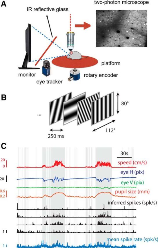
Experimental setup. A, Activity of cells in V1 was imaged while a mouse, on a freely rotating platform, observed a continuous visual stimulus. The head was horizontal. B, Sample of a visual stimulus sequence. The stimulus consisted of a pseudorandom sequence of gratings drawn from a Hartley basis set presented at a rate of 4 frames/s. C, Segment of a data record depicting platform speed, eye position, pupil size, the inferred spikes of four sample cells, and the mean spike rate of the population. Gray bars in this and subsequent figures indicate periods of locomotion defined by a threshold on the speed signal.

Visual stimulation

Hartley stimuli (Ringach et al., 1997; Malone and Ringach, 2008) were generated in real time by a processing sketch using OpenGL shaders (see http://processing.org). The stimulus was updated 4 times/s on a BenQ XL2720Z screen refreshed at 60 Hz. The screen measured 60 cm by 34 cm and was viewed at a 20 cm distance, thereby subtending 112 × 80 degrees of visual angle. The maximum spatial frequency was 0.15 cycles/°, which corresponds to 12 cycles along the vertical extent of the display. The Hartley set consisted of the following gratings:

where cas(x) ≡ cos(x) + sin(x) and the wavenumbers k_x and k_y represent the number of cycles along the horizontal and vertical axes, respectively, and these indices ran between −12 and 12, excluding the origin (k_x, k_y) = (0, 0). Therefore, the total number of different images in the Hartley set was ((2 × 12 + 1)² − 1) × 2 = 1248. The responses to the four spatial phases that are present at each combination of orientation and spatial frequency were averaged, leading to 312 locations in the orientation and spatial frequency domain. Each combination was presented, on average, 15.4 times during a 20-minute-long stimulus refreshed at 4 Hz. This stimulus update rate was selected in an attempt to collect data as fast as possible while still evoking reliable responses from cells.

A transistor-transistor logic pulse was generated by an Arduino board at each stimulus update transition. The pulse was sampled by the microscope and time stamped with the frame and line number being scanned at that time. The time stamps provided a way to align the visual stimulation and imaging data in time.

The screen was calibrated using a Photo-Research PR-650 spectro-radiometer and the result used to generate the appropriate gamma corrections for the red, green, and blue components via an nVidia Quadro K4000 graphics card. The contrast of the stimulus was 99%. The center of the monitor was positioned with the center of the receptive field population for the eye contralateral to the cortical hemisphere under consideration. The location of the receptive fields were estimated by an automated process in which localized, flickering checkerboard patches appeared at randomized locations within the screen. This experiment was run at the beginning of each imaging session to ensure the centering of receptive fields on the screen.

Data processing

Motion stabilization.

Calcium images were aligned to correct for motion artifacts in a two-step process. First, images were aligned rigidly in a recursive fashion to correct for slow drifts in the imaging plane. Pairs of neighboring images in time were aligned by finding the peak of their cross-correlation and then pairs of averages of such pairs were aligned and so on. In the second step, images were aligned nonrigidly to a reference mean image to correct for fast in-plane movements, which are frequently observed during grooming. The Lucas–Kanade algorithm was applied iteratively (Greenberg and Kerr, 2009) to match a reference mean image nonrigidly, refining the estimate of this reference mean image after each alignment iteration.

Segmentation.

After motion stabilization, a MATLAB (The MathWorks) graphical user interface tool developed in our laboratory was used to define regions of interest corresponding to putative cell bodies manually. Correlation and kurtosis images were used to identify cell candidates (Smith and Häusser, 2010). The correlation image, corresponding to the average correlation of a pixel and its eight neighbors across time, highlighted regions of space that covary in time. The kurtosis image highlights regions in space with signals composed of large, infrequent deviations: putative spikes. These images were computed after subtracting linear trends (Pnevmatikakis et al., 2014).

These images were used to identify approximately circular regions of space of an appropriate radius visually with high correlation and high kurtosis. Clicking a seed pixel at the center of such a candidate patch allowed the definition of a region of interest by flood filling an image corresponding to the correlation of the highlighted pixel and every other pixel in the image field (Ozden et al., 2008). The interface then allowed the user to grow or shrink the region of interest dynamically to a desired size.

Signal extraction and spike inference.

After segmentation, signals were extracted by computing the mean of the calcium fluorescence within each region of interest. Non-negative deconvolution (Vogelstein et al., 2010; Pnevmatikakis et al., 2014) was used to estimate spikes from calcium traces. The inverse, constrained form of the non-negative deconvolution problem was solved (Pnevmatikakis et al., 2014) using the CVX package (Boyd and Vandenberghe, 2004). To mitigate the effect of drifting background fluorescence, the offset was modeled as slowly moving in time with a 10-knot cubic spline. The noise of the measured calcium signals was estimated as the median absolute deviation of the first-order derivative divided by a factor of $.6745\sqrt{2}\approx .954$ (Johnstone and Silverman, 1997).

The constrained deconvolution method of Pnevmatikakis et al. (2014) requires the specification of the impulse response of the calcium indicator. An exponential impulse response function was assumed and its decay time estimated using reference data consisting of simultaneous loose-seal cell-attached recordings and calcium imaging of GCaMP6f in visual neurons (Chen et al., 2013). This dataset was resampled at a sampling rate of 15.5 Hz, non-negative deconvolution was run for a grid of values of decay times, the R² of the estimated calcium signal and the ground-truth cell spike trains across the 11 cells of the dataset were calculated, and the parameter set with the largest mean R² was selected. This yielded a decay time τ_1/2 = 135 ms, for a validated mean R² of 0.42 (cf. supplemental Table 3 in Chen et al., 2013). Our analyses and the resulting interpretation assume that there is an approximately linear relationship between the inferred spike rate and the actual spike rates from the neurons, as partly justified by existing data (see Fig. 3E in Chen et al., 2013).

Figure 3.

Relative gain depends on preferred spatial frequency and orientation. A, Relative gain increases with preferred spatial frequency. The population was split into three groups preferring low (0 < ω < 0.025 cycles/°), medium (0.025 < ω ≥ 0.075 cycles/°), and high (ω > 0.075 cycles/°) spatial frequencies. Mean relative gain (error bars are bootstrapped 95% confidence intervals) is shown for each group. There is an evident dependence of relative gain on the preferred spatial frequency of neurons. B, Relative gain is correlated with preferred spatial frequency. This is the same data as in A replotted without binning to convey the degree of variability. Red line is best linear fit. C, Dependence of relative gain with orientation. There is a moderate tendency for relative gain to be larger at oblique orientations. D, Distribution of eye velocity during the experiments (color code is in a log scale). Although most of the time the eyes are still, when they move, they tend to do so along the horizontal axis. The frequency of such movements is higher during locomotion (Fig. 1C).

Generic linear model

The response of a neuron to a stimulus was assumed to be given by the following linear model:

where ϵ(t) is independent, identically distributed Gaussian noise, s(ω_x, ω_y, t) is the stimulus presented at time t, w(ω_x, ω_y) is the Fourier kernel, v(τ) is the temporal kernel, b is the offset during rest, a is the change in offset during locomotion, y(t) is the measured response, and r(t) is an indicator variable taking the value 1 when the instantaneous velocity of the animal is at least 1 cm/s and zero otherwise. The parameter a in the equation allows for shifts in the baseline as a function of state.

This model was fit through alternating least-squares (Ahrens et al., 2008) and the norm of the temporal kernel was constrained to 1. A smoothness penalty was used for the spatial kernel (Wu et al., 2006) and its strength was determined by fivefold cross-validation.

The quality of fit of this generic linear model was compared with a baseline model as follows:

A fit was considered significant whenever the cross-validated sum-of-squared error SSE_L of the generic linear model was such that:

where SSE_B corresponds to the sum-of-squared error of the baseline model and r_L is analogous to a correlation (Pearson's r) value. A total of 3803/7018 (54.2%) neurons were significantly tuned according to this criterion.

Parametric linear model

To estimate the preferred spatial frequency and orientation, as well as their respective bandwidth, a parametric linear model was fit as follows:

where the Fourier kernel is a separable function in orientation and spatial frequency. The orientation tuning is a von Mises function and the spatial frequency tuning is a log-Gaussian function. The parameter r = $\sqrt{{\omega }_x^2+{\omega }_y^2}$ represents the optimal spatial frequency and θ = arctan(ω_y/ω_x) the optimal orientation. The parameter A_θ controls the sharpness of tuning in the orientation domain and σ_r controls the sharpness of tuning in spatial frequency. This model was fit through alternating nonlinear least-squares using the solution to the generic linear model as a seed for the temporal kernel and an initial grid search to find optimal values for r, θ, σ_r, A_θ. A total of 3476/7018 (49.5%) neurons were considered significant (r > 0.15).

Separable linear models

In some analyses, the gain of the linear model was quantified as a function of state by fitting the linear model as follows:

where cr(t) + d correspond to the state-dependent gain. The gain during locomotion is then given by c + d and the gain during rest is d. The relative gain change from rest to locomotion, from the model parameters, is given by 1 + c/d. The relative gain is analogous to the concept of an attentional field (Reynolds and Heeger, 2009). The model was fit through alternating least-squares and declared significant if it attained a cross-validated r-value of 0.15 attained by 3861/7018 (55.0%) of neurons.

Inseparable linear models

In one instance (see Fig. 2D,E), spatial and temporal kernels were allowed to depend on whether the animal was in locomotion or rest. Therefore, the generic and parametric linear models of the previous sections were fit contingent on whether the animal was undergoing locomotion (criterion: instantaneous velocity of 1 cm/s). The factor ar(t) was ignored in this case. Fits were declared significant if the model could achieve a cross-validated correlation value of at least 0.15 in both the rest and locomotion conditions in 2605/7018 (37.1%) neurons.

Figure 2.

Effect of behavioral state on the tuning of V1 neurons in the orientation and spatial-frequency (Fourier) plane. A, Tuning of four sample cells in the Fourier domain (origin is at the center) and their corresponding temporal kernels (bottom). These estimates were obtained by fitting a linear model to the data (Materials and Methods, Eq. 2). All temporal kernels are shown starting at t = 0. Spatial frequency along the horizontal meridian is represented by ω_x and the spatial frequency along the vertical meridian by ω_y. All Fourier kernels share the same pseudocolor scale. Positive values (red hues) represent stimuli with orientation and spatial frequency that led to increases in the response of the cell; negative values (blue hues) represent stimuli that suppressed the response of the cell; neutral stimuli are represented by a green hue. B, Distribution of peak kernel positions in the Fourier domain across the population. The distribution is symmetric because the Fourier kernel is symmetric. C, Top, Distribution of preferred orientations, θ. Bottom, Distribution of preferred spatial frequencies, ω = $\sqrt{{\omega }_x^2+{\omega }_y^2}$. The symmetry of preferred orientations is a consequence of the symmetry of the Fourier kernels as well. Only well fit neurons (cross-validated r > 0.15, n = 3476; see Materials and Methods for details) are considered in this analysis. D, Tuning of four sample cells in the Fourier domain during rest (top) and locomotion (bottom). Temporal responses are shown in the middle (blue: rest, red: locomotion). This was obtained by fitting a model that allowed changes in gain between locomotion and rest (Materials and Methods, Eq. 6). E, Preferred spatial frequency and orientation are largely preserved across states. F, Response gain increases substantially during locomotion. G, There is a small but significant increase in baseline firing rate of 0.12 ± 0.01 SDs of the response during locomotion (p < 0.001, bootstrap test).

Bayesian decoder

Poisson independent decoder.

To examine how locomotion influences the representation of stimuli, the framework of Jazayeri and Movshon (2006) was followed. A brief overview of the framework is provided here. The goal is to decode the stimulus by estimating the probability that a population response was generated by a given stimulus θ_j out of a finite range of possibilities, p(θ = θ_j). It was assumed that the i-th of N neurons has a tuning curve f_i(θ) and that, on a given trial, n_i spikes were observed from this neuron. Assuming that each neuron follows independent Poisson statistics and that each stimulus is equally likely, it follows from Bayes' theorem that:

Taking the log and removing the normalization constant, which is independent of θ, the following is found:

From this, the properly normalized distribution is recovered as follows:

The log-likelihood L(θ_j) can be computed straightforwardly as the sum of the log of tuning curves weighted by the number of spikes measured from each neuron, with an offset to compensate for biases in the population representation. It is possible to construct a two-layer neural network carrying equivalent information to L(θ_j) (Jazayeri and Movshon, 2006) and a point estimate corresponding to the maximum likelihood estimate of the stimulus can be obtained by a recurrent network (Deneve et al., 1999).

Homogeneous gain increase.

The effect that a homogenous gain increase has on population decoding will now be discussed. The SD of a Poisson neuron is proportional to the square root of its mean; signal-to-noise ratio thus increases when the rate of a neuron increases. Intuitively, therefore, if a population of Poisson-like neurons increases their gain by a common factor in response to a change of state, then decoding should be facilitated.

Under the Poisson-independent decoder, a homogeneous gain of α has the effect of multiplying the log-likelihood (Eq. 8) by a factor α. It follows from Equation 9 that, under an increase in gain, probabilities therefore become more extreme: p(θ = θ_j) values that were most likely before the gain increase become still more likely after gain increase and values that were less likely become still less likely. Therefore, an increase in gain across the board decreases the uncertainty of the decoder and, because the decoder is unbiased, this implies that decoding error decreases when gain increases.

Nuisance factor

Now suppose, more generally, that neurons are modulated by a nuisance factor φ not relevant to decoding the parameter of interest; for example, locomotion, contrast, etc. Then, tuning curves become a function of both the parameter of interest and the nuisance factor:

Assuming that the nuisance factor modulates tuning curves in an arbitrary fashion, then a different decoder must be used for every value of the nuisance parameter; equivalently, one decoder of the form in Equation 8, can be used, with synaptic weights modulated dynamically by the nuisance parameter. In either case, downstream decoding becomes more complicated. However, if modulation is multiplicative, that is, tuning curves are separable, then:

In this case L(θ_j) has a very simple form:

where k is independent of φ. Equation 12 shows that, when the nuisance parameter modulates tuning curves multiplicatively, the stimulus can be decoded in exactly the same way as before except that the offset b(θ₀, φ) now changes with φ.

Empirical decoder

Graf et al. (2011) showed that the theoretical decoder of the previous section can underperform when the population has correlated noise or does not follow Poisson statistics exactly. Equation 12 can be relaxed to compensate for these deviations from the theoretical model. Factors corresponding to log tuning curves are replaced with empirically derived weights as follows:

Absorbing the offset into a design matrix x, this linear model for the likelihood can be rewritten into the canonical form:

As highlighted previously, this non-normalized log-likelihood can be transformed to a normalized likelihood by the softmax transformation:

Finally, under this model, μ is the probability distribution of the categorical stimulus variable y and it follows that it has a multinomial distribution:

Therefore, this this empirical decoder can be interpreted as a special instance of multinomial regression, itself a special case of generalized linear models (McCullagh and Nelder, 1989).

Decoder variants, fitting, and validation

To measure how locomotion modulates decoding accuracy, both theoretical and empirical decoders were fit to the data.

In the case of the theoretical decoder, the number of spikes in a three-frame window centered on the mean temporal latency of all cells within an experiment were counted. The tuning curves smoothed by a Gaussian kernel were then computed to derive model weights. The size of the smoothing kernel was determined by minimizing the fivefold cross-validation decoding error. This decoding error was derived by selecting maximum likelihood (ML) estimates under the model and computing their root mean squared error (RMSE) relative to the actual stimuli in Fourier space.

For the empirical decoder, model weights were estimated by maximum a posteriori estimation through convex optimization in the framework of generalized linear models (McCullagh and Nelder, 1989). Rather than directly counting spikes, the model was allowed to have a continuous temporal window, which was learned from the data using alternating optimization. A smoothness penalty on the log-tuning curves with strength determined by fivefold cross-validation was used. As with the theoretical decoder, the RMSE was computed for the maximum likelihood estimates. In addition, the RMSE for a Bayesian point estimate, which uses the whole estimated probability distribution, and not simply its maximum, was computed to minimize the expected RMSE.

Decoding was more accurate during locomotion for theoretical, empirical ML, and empirical Bayesian decoders; in absolute terms, the empirical Bayesian decoder outperformed the empirical ML, which outperformed the theoretical decoder. In Figure 5, the results of the more familiar empirical ML decoder are shown.

Figure 5.

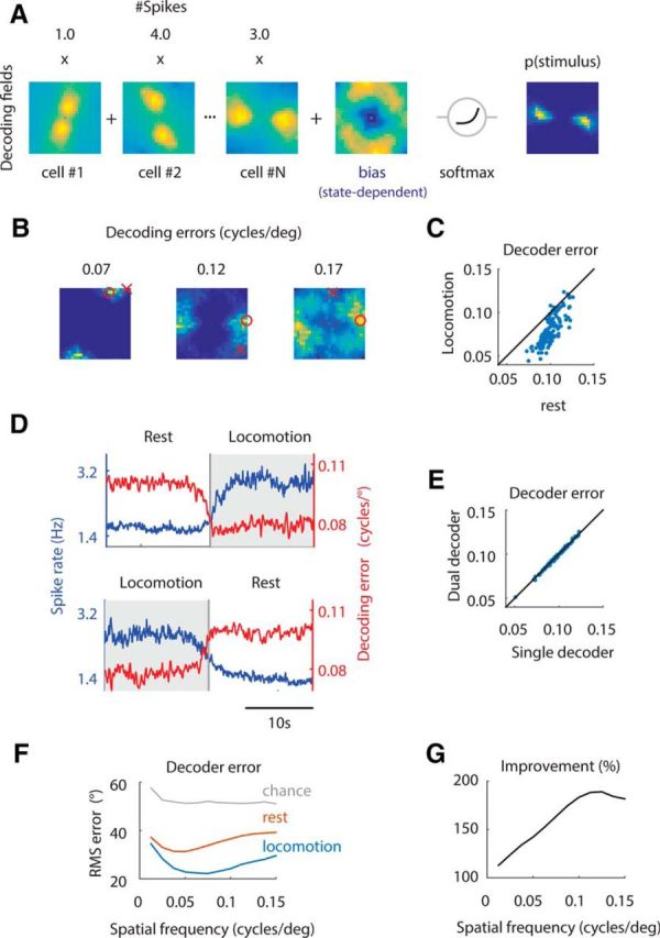
Locomotion enhances the population code and the cortical representation of high spatial frequencies. A, The decoder consisted of the linear weighting of decoding fields by spike rates over the Fourier domain plus a state-dependent bias term, followed by a soft-max nonlinearity (Materials and Methods). The result is an estimate of the probability of the stimulus given the population firing rate, p_(stimulus). B, Examples of p_(stimulus), along with the estimated (red circle) and presented (red cross) stimuli together with the decoding error measured as the Euclidean distance between these two points on the Fourier plane. C, Decoding error is smaller during locomotion compared with during rest. D, Average changes in population spike rate and decoding error during transitions from rest to locomotion (top) and from locomotion to rest (bottom). E, A single decoder that only modifies the bias in a state-dependent manner performs as well as two separate decoders for each state. In other words, there is no increase in performance if we allow the model to fit different Fourier kernels during locomotion and rest. F, Decoding of orientation as a function of behavioral state and spatial frequency. Gray line represents chance performance. The lowest decoding errors are achieved during locomotion. G, Relative improvement of decoder performance during locomotion versus rest. The relative improvement, in percentage, is defined as 100 * (RMS_loc − RMS_chance)/(RMS_rest − RMS_chance). The relative improvement in decoding accuracy is concentrated at high spatial frequencies, where gain increases are more pronounced.

To verify that the improved stimulus representation could be used advantageously by a simple decoder in which behavioral state only modifies the prior, separate decoders were also fit for the rest and locomotion states using the same criteria as previous analyses. At prediction time, the prediction of the decoder relevant to the current state was used. Figure 5 shows that the decoding accuracy was very similar between these more complex, dual decoders and the single “efference copy” decoder, as measured by the empirical ML error. Similar results were obtained for the theoretical and empirical Bayesian decoders (data not shown).

Decoding accuracy as a function of spatial frequency

The same empirical decoders described in the previous section were used to examine the dependence of the decoding accuracy on spatial frequency and state (see Fig. 5). The ability of the model to predict the probability of the orientation of the stimulus given the absolute spatial frequency and spike trains was assessed as follows:

However, the model actually defines:

The probability distribution (Eq. 17) was approximated by considering a small range of spatial frequencies around the target spatial frequency:

where α corresponds to the range of spatial frequencies around the one considered, which was set to 0.0125 cycles/°. Both ML and Bayesian variants of this model were considered; Bayesian variants performed better, but otherwise, the main quantitative effects (see Fig. 5) were similar in both variants. The Bayesian variant was used for the data shown in Figure 5.

Motion onset analysis

To measure the temporal relationship between motion onset, decoding accuracy, and firing rate, transitions between locomotion and rest were estimated as follows. An onset period was defined as one in which movement was slower than 0.7 cm/s in 75% of time periods in the preceding 5 s and faster than 1 cm/s in the 75% of time periods in the 5 s following. Onset times were defined as the centers of onset periods, discarding onset times separated by <15 s. Computed mean firing rate and RMSE around the time of locomotion onset were then computed. Offset times were defined similarly.

Derivation of the gain of an exponential nonlinearity with a normal input

Assume we have an exponential nonlinearity of the form r = A exp(λx), where the input is normally distributed x ∼ N(μ, σ) (see Fig. 4B). Then, the slope of the best linear fit between the input and output was computed as: g = (E{r x} − E{r}E{x})/σ². The terms in this equation can be calculated as follows:

After substituting in the expression for the gain, the following is obtained:

By using Equation 21, the expression can be seen to be equal to g = λr̄. In other words, the gain is proportional to the mean rate.

Figure 4.

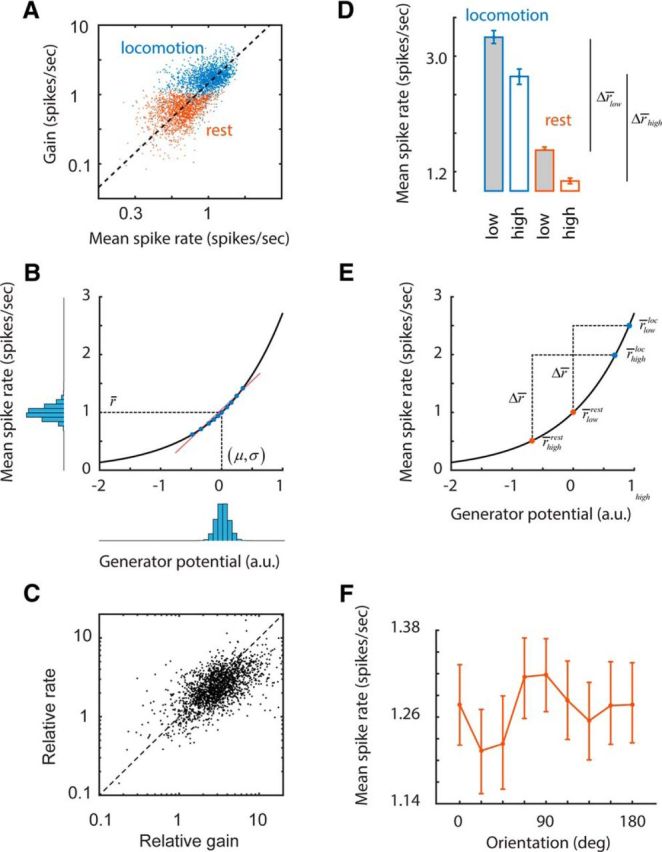
Changes in the operating point of neurons may explain differential gain changes. A, Scatter plot of the mean rate and gain of cells during periods of rest and locomotion. The dashed line represents the best linear fit. B, An exponential spiking nonlinearity with a Gaussian input has the property that the mean response is proportional to the gain, consistent with the data in A. Here, r̄ represents the mean spike rate and (μ, σ) represent the mean and SD of the generator potential. The blue filled dots represent a small subset of data of the joint distribution of the generator potential and the mean spike rate as related by the nonlinearity. The red line represents the best linear fit to these points. The slope of this line is the gain. C, As predicted by this simple rectification model, relative changes in gain are closely related to relative changes in mean spike rate. D, Cells with low- and high-spatial-frequency preferences have different operating points during rest and locomotion. The relative ordering of these rates, along with the approximate identity relationship shown in C, explain how differential gain increases may occur. E, Graphic summary of the relationship in D depicting the relative positioning of operating points of cells with low- and high-spatial-frequency preferences along the spiking nonlinearity. F, There is a trend of mean rate with orientation that complements the dependence of relative gain with orientation (Fig. 3B), consistent with the proposed explanation based on the shifts of the operating points.

Results

To determine whether the representation of the image in V1 changes between locomotion and rest, we placed mice on a freely rotating platform and measured changes in the fluorescence of V1 pyramidal neurons expressing GCaMP6f (Chen et al., 2013) using two-photon laser scanning excitation (Fig. 1A). Mice were presented with a 20-min-long sequence of high-contrast, sinusoidal gratings that had random orientations and spatial frequencies (Hartley basis functions) refreshed at a rate of 4 Hz (Ringach et al., 1997; Malone and Ringach, 2008; Fig. 1B). During these sessions, mice spontaneously switched between periods of rest and locomotion (Fig. 1C). Such transitions were marked by correlated changes in platform velocity, the rate of horizontal eye saccades, pupil size, and mean population firing rate (Fig. 1C; Niell and Stryker, 2010; Polack et al., 2013; Erisken et al., 2014).

A continuous visual stimulation with constant mean luminance and contrast was selected to prevent external visual events from inducing changes in cortical state (Tan et al., 2014) while allowing us to map the tuning of cells. The relatively fast rate and unpredictability of the stimulus sequence helped keep sensory mismatch between the visual and motor signals at a constant level, likely alleviating its influence on V1 activity (Keller et al., 2012). Moreover, the stimulus sequence consisted of flashed gratings and contained no net motion, thereby minimizing the contribution of visual speed to the activity of neurons (Saleem et al., 2013).

From the responses of neurons to the Hartley sequence, we estimated the tuning of each cell in the joint spatial-frequency and orientation domain and their temporal responses via linear regression (Fig. 2A; Materials and Methods, Eq. 2). Many neurons were responsive to the stimulus sequence (defined as a cross-validated r > 0.15 in 3803/7018 or 54.2% of the cells). To capture the preferences of neurons for orientation and spatial frequency, we fit a parametric model consisting of separable von Mises tuning for orientation and log-Gaussian spatial frequency tuning (Materials and Methods, Eq. 5). Although most neurons were tuned to low spatial frequencies, a large range of preferences was observed, as noted by the distribution of their preferred parameters in the Fourier plane (Fig. 2B,C). A few neurons preferred spatial frequencies close to or beyond the largest tested (0.15 cycles/°; Fig. 2C, bottom).

To examine the effect of behavioral state on the tuning properties of individual neurons, we estimated receptive fields for periods of locomotion (defined by a platform speed >1 cm/s) and rest (speed <1 cm/s) separately. Temporal kernels were constrained to have unit norm in both locomotion and resting states. Therefore, any changes in gain were represented by changes in the amplitude of the Fourier kernels.

Consistent with prior studies, we found that locomotion led to increases in gain (Fig. 2D; Niell and Stryker, 2010; Bennett et al., 2013; Polack et al., 2013). We define the ratio between the gain during locomotion and the gain during rest as the “relative gain.” Preferred orientation and spatial frequency were largely preserved between locomotion and resting states (Fig. 2E). To investigate the behavior of the relative gain in more detail, we fit a model with a single tuning curve, but allowed for variations in baseline firing rate and gain across locomotion and rest states (see Materials and Methods, Eq. 6). We found that the relative gain across the population was 2.7 ± 0.1 (Fig. 2F, geometric mean, p < 0.001, bootstrap test). There was a small but significant increase in baseline firing rate of 0.12 ± 0.01 SDs of the response (Fig. 2G, p < 0.001, bootstrap test).

Next, we investigated whether the relative gain was dependent on the preferred stimulus parameters of the neurons. Indeed, we found that relative gain was largest for cells preferring high spatial frequencies (Fig. 3A). The relative gain for neurons preferring high spatial frequencies (ω > 0.075 cycles/°, n = 784) was 3.1 ± 0.15 (mean ± 95% confidence interval), which was higher than for cells preferring medium (0.025 < ω ≤ 0.075 cycles/°, 2.7 ± 0.1, n = 654) and low spatial frequencies (0 < ω < 0.025 cycles/°, 2.45 ± 0.08, n = 388). In other words, neurons with high preferred spatial frequencies experienced relative gains ∼26% larger than cells tuned to the low spatial frequencies. A scatter plot of the same data captures the variability in the population (Fig. 3B). Even though this may appear to be a modest difference at first sight, we show below that this phenomenon has a marked effect on the ability of the entire population to encode high spatial-frequency information.

Although preferred spatial frequency was the major factor related to relative gain increase, we also observed a weaker modulation of relative gain with respect to preferred orientation (Fig. 3C). Curiously, the data hinted at larger relative gains at oblique orientations. To investigate whether there was a relationship between this trend and eye movements during the experiments, we computed the distribution of eye velocities, which showed a clear bias toward the horizontal (Fig. 3D), consistent with prior studies (Bennett et al., 2013). If an increase in horizontal retinal motion led to higher responses during locomotion, we would expect relative gain to be maximal in cells tuned to vertical orientations. However, there was no obvious peak at that location (Fig. 3C). Its absence suggests that eye movements and the resulting retinal slip are not a major contributor to increases in relative gain. In addition, we verified there are no major changes in eye torsion between rest and locomotion (Movies 1 and 2). An alternative explanation for this peculiar trend is offered below.

Movie 1.

Example of the measurement of pupil size and torsional eye movements during locomotion. The red bar represents normalized, instantaneous running speed. Torsion is measured as the angle formed by the line joining the center of the pupil and a selected two-dimensional feature of the iris and the horizontal axis in the image plane. While the pupil dilates during locomotion, torsion remains approximately constant.

Movie 2.

Another example of changes in pupil size and torsion during locomotion. The information is presented in the same format as in Movie 1.

An important observation, which led us to propose a possible mechanism for the observed changes in gain, was the existence of an approximately linear relationship between gain and mean firing rates of neurons (Fig. 4A). This relationship arises if one postulates an exponential, spiking nonlinearity r = Aexp(λx), linking the response of the cell r to a generator potential x (Fig. 4B; Granit, 1955; Nykamp and Ringach, 2002; Ringach and Malone, 2007). If we assume the generator potential is normally distributed with mean μ and SD σ, then the mean spike rate is given by:

Moreover, it can be shown that the gain, which corresponds to the linear regression coefficient between the response and the generator potential, is simply g = λr̄ (see derivation in Materials and Methods). In other words, the gain is proportional to the mean response, consistent with the experimental observation (Fig. 4A).

If changes in gain reflect changes in the operating point of the cells between locomotion and rest (Bennett et al., 2013; Polack et al., 2013), then this simple model predicts that the relative gain across two states must be equal to the relative change in mean response, g_loc/g_rest = r̄_loc/r̄_rest. Where g_{loc,rest} represents the gain during locomotion and rest, respectively, and we use a similar notation for the mean spike rates, r̄_{loc,rest}. Remarkably, this relationship holds reasonably well in our data (r = 0.62, p < 10⁻¹⁰; Fig. 4C).

In addition, if shifts in the operating points along a spiking nonlinearity explain changes in gain, it is possible that the difference in relative gain shown by neurons with high and low spatial frequency preferences is due to their operating points shifting in different ways. First, we find that cells with high spatial frequency preference have lower spiking rates than cells with low spatial frequency preference during both rest and locomotion (Fig. 4D). Second, increases in absolute firing rates between rest and locomotion experienced by these two groups are statistically indistinguishable, Δr̄_low ≈ Δr̄_high = Δr̄ (rank-sum test, p > 0.32; Fig. 4D).

A graphic summary of these relationships helps to explain how the differential changes in gain between rest and locomotion may arise from the different operating points of the neurons (Fig. 4E). In the figure, r̄_{low,high}^{rest,loc} represent the mean rates of the two cell groups during rest and locomotion, and Δr̄ is the increase in firing rate in the two groups between rest and locomotion. Then, according to the model:

and a similar relationship holds for the group of cells with high spatial frequency preference:

However, the data show that the operating points during rest differ, such that r̄_rest^low > r̄_rest^high, implying that:

In other words, the relative gain for cells with low spatial frequency preference is smaller than the group with high spatial frequency preference.

Armed with these observations, we return to the puzzling dependence of relative gain changes with orientation (Fig. 3B). If our proposed explanation is correct, then we should expect to see a matching dependence of the operating point with orientation preference as well. Indeed, we see a tendency for cells with preferred orientations around vertical and horizontal to show larger firing rates during rest than cells tuned to the oblique orientations (Fig. 4F). Such trends can cause cells tuned for vertical and horizontal to experience smaller increases in gain than cells tuned to the oblique orientations, which is what is observed in the data (Fig. 3B). Altogether, these analyses indicate that the change in gain experienced by a neuron is tightly linked to the shift in its operating point between behavioral states, which, in turn, depends on its preferred spatial frequency and orientation.

Is the change in gain during locomotion sufficient to have an effect on the representation of visual information in V1? As gain (and consequently the signal-to-noise ratio of individual cells) increases during locomotion, the ability of an ideal observer to predict the stimuli that triggered a population response is expected to improve as well (see Materials and Methods). Moreover, if changes in state only modify the gain of individual cells while leaving their tuning invariant, the stimulus can be decoded in a manner where the behavioral state (rest or locomotion) only modifies the prior probability of stimuli (see Materials and Methods).

To verify this prediction using the collected data, we trained a Bayesian decoder to estimate the visual input from population activity (Graf et al., 2011; Fig. 5A). The decoder computed a spike-weighted sum of decoding fields to yield an estimate of the probability that the population response was generated by a given stimulus. The resulting distribution led to an estimate of a stimulus in the Fourier domain, from which we assessed the decoding error (Fig. 5B).

Population activity represented stimuli much more accurately during locomotion than during rest. The decoding error was strongly reduced during periods of locomotion relative to rest (Fig. 5C). Decoding error decreased rapidly after the onset of locomotion and increased more gradually before a transition to rest, indicating that the modulation was strongly locked to changes in mean spike rate and behavioral state (Fig. 5D). Importantly, using two separate decoders during locomotion and rest did not improve prediction errors (Fig. 5E). This indicates that the population can be appropriately modeled by a fixed set of kernels that change solely in gain and that the change approximately behavioral state is adequately captured by changes in the prior distribution (see Materials and Methods).

Finally, we determined whether the preferential enhancement found for cells tuned to high spatial frequencies could support enhanced spatial resolution in the V1 population. We repeated the decoding analysis, focusing on orientation decoding as a function of behavioral state and spatial frequency. Across all spatial frequencies, orientation was decoded more accurately during locomotion (Fig. 5F). However, the improvement relative to rest, using chance performance as the baseline, was more pronounced at high spatial frequencies (Fig. 5G).

Discussion

Previous research has shown that evoked firing rates increase and the detectability of weak stimuli improve during locomotion compared with rest (Niell and Stryker, 2010; Bennett et al., 2013; Polack et al., 2013). Our analyses indicate that individual cells modulate their gain in a way consistent with a shift in their operating point along an exponential nonlinearity. This explains the approximately linear relationship between gain and mean response rate (Fig. 4). An exponential nonlinearity was chosen because it is amenable to mathematical treatment and facilitates the explanation of how shifts in operating point modulate gain. Other accelerating nonlinearities, such as half-squaring, can also generate an approximate linear relationship between gain and mean rate over an adequate range of inputs. To study these issues in more detail, it would be important to measure the dependence between the operating point and preferred stimulus parameters, as well as the shape of spiking nonlinearities, using intracellular recording techniques (Bennett et al., 2013; Polack et al., 2013; Tan et al., 2014).

The cortical circuit involved in modulating the operating point remains to be explored. Growing evidence indicates that, during periods of locomotion, VIP interneurons (cells expressing the vasoactive intestinal polypeptide) increase their firing rates and inhibit SOM interneurons (somatostatin-expressing inhibitory neurons; Fu et al., 2014). SOM-expressing cells have been implicated as the source of surround suppression in pyramidal neurons (PYR; Adesnik et al., 2012). The disinhibition resulting from the activation of the VIP → SOM→PYR circuit would explain the increase in spatial summation (Ayaz et al., 2013), the shift of operating points toward more depolarized states during locomotion compared with rest (Bennett et al., 2013; Polack et al., 2013), and the resulting increase in gain during locomotion.

Expanding on previous findings, we found that relative gain is not uniform across the population, but depends on the tuning preferences of the neurons (Fig. 3). The most salient effect is that neurons with a preference for high spatial frequencies have relative gains 25% larger than those tuned for small spatial frequencies. A decoding analysis showed that, during locomotion, there is an enhanced visual representation that supports better discriminability of high-contrast stimuli, in particular stimuli at high spatial frequencies (Fig. 5).

Although arbitrary state-dependent changes in tuning could make the neural code ambiguous and difficult to read, a simple downstream decoder can read out cortical signals efficiently when only gain is modulated and receptive field tuning curves are approximately invariant. In this way, increased resources (neuronal action potentials and their corresponding metabolic cost) can be deployed during moments of high behavioral demand such as locomotion, improving the representation of relevant stimuli (Lennie, 2003). Therefore, the neuronal code is shaped adaptively to increase spatial resolution in V1 without increasing the complexity or burden of decoding in downstream areas.

The preferential enhancement of high-spatial-frequency information lends additional support to the idea that changes in V1 during periods of increased alertness and locomotion in rodents resemble the changes that occur in nonhuman primates during the allocation of spatial attention (Harris and Thiele, 2011). Specifically, the allocation of spatial attention in human subjects leads to increased spatial resolution, an effect that has been hypothesized to be driven by a selective increase in response gain at high spatial frequencies (Anton-Erxleben and Carrasco, 2013). We found that such an effect is evident in mouse V1, where differential gain modulation enhances the representation of high spatial frequencies during increased levels of alertness and locomotion. The evolutionary advantage of such enhancement is unclear. During locomotion, one expects the retinal image to become blurred by motion (Barlow and Olshausen, 2004). This might be particularly problematic in species that are unable to stabilize the retinal image by ocular tracking of external targets, such as mice. Perhaps the preferential enhancement of high spatial frequencies evolved as a way to counteract such loss of information during self-motion relative to a stationary environment.

Our findings indicate that the dependence of relative gain on the preferred tuning parameters of neurons is linked to corresponding differences in how their operating points shift across states. During rest, cells with a preference for high spatial frequency have smaller mean responses and gains than cells with a preference for low spatial frequency (Fig. 4). How this relationship arises remains unknown and we can only speculate at this point. One possibility is that the spatial distribution of the geniculate inputs required to generate a band-pass filter with a high-spatial-frequency preference involves the pooling of ON and OFF center cells to generate the ON and OFF subregions of simple cells. In contrast, cells with low-pass-spatial frequency profiles may be dominated by a fewer number of inputs from geniculate cells with the same center sign. One could conjecture that cells with balanced ON/OFF inputs and high-spatial-frequency selectivity are in a higher conductance resting state (and lower gain) than their counterparts with low-spatial-frequency selectivity. Therefore, the difference in the operating points may be a consequence of the number of synaptic inputs required to make up the corresponding receptive fields.

References

- Adesnik H, Bruns W, Taniguchi H, Huang ZJ, Scanziani M. A neural circuit for spatial summation in visual cortex. Nature. 2012;490:226–231. doi: 10.1038/nature11526. [DOI] [PMC free article] [PubMed] [Google Scholar]
- Ahrens MB, Paninski L, Sahani M. Inferring input nonlinearities in neural encoding models. Network. 2008;19:35–67. doi: 10.1080/09548980701813936. [DOI] [PubMed] [Google Scholar]
- Anton-Erxleben K, Carrasco M. Attentional enhancement of spatial resolution: linking behavioural and neurophysiological evidence. Nat Rev Neurosci. 2013;14:188–200. doi: 10.1038/nrn3443. [DOI] [PMC free article] [PubMed] [Google Scholar]
- Arroyo S, Bennett C, Hestrin S. Nicotinic modulation of cortical circuits. Front Neural Circuits. 2014;8:30. doi: 10.3389/fncir.2014.00030. [DOI] [PMC free article] [PubMed] [Google Scholar]
- Ayaz A, Saleem AB, Schölvinck ML, Carandini M. Locomotion controls spatial integration in mouse visual cortex. Curr Biol. 2013;23:890–894. doi: 10.1016/j.cub.2013.04.012. [DOI] [PMC free article] [PubMed] [Google Scholar]
- Barlow HB, Olshausen BA. Convergent evidence for the visual analysis of optic flow through anisotropic attenuation of high spatial frequencies. J Vis. 2004;4:415–426. doi: 10.1167/4.8.415. [DOI] [PubMed] [Google Scholar]
- Beatty J. Task-evoked pupillary responses, processing load, and the structure of processing resources. Psychol Bull. 1982;91:276–292. doi: 10.1037/0033-2909.91.2.276. [DOI] [PubMed] [Google Scholar]
- Bennett C, Arroyo S, Hestrin S. Subthreshold mechanisms underlying state-dependent modulation of visual responses. Neuron. 2013;80:350–357. doi: 10.1016/j.neuron.2013.08.007. [DOI] [PMC free article] [PubMed] [Google Scholar]
- Bereshpolova Y, Stoelzel CR, Zhuang J, Amitai Y, Alonso JM, Swadlow HA. Getting drowsy? Alert/nonalert transitions and visual thalamocortical network dynamics. J Neurosci. 2011;31:17480–17487. doi: 10.1523/JNEUROSCI.2262-11.2011. [DOI] [PMC free article] [PubMed] [Google Scholar]
- Boyd S, Vandenberghe L. Convex optimization. Cambridge: Cambridge University; 2004. [Google Scholar]
- Carrasco M, Barbot A. How attention affects spatial resolution. Cold Spring Harb Symp Quant Biol. 2014;79:149–160. doi: 10.1101/sqb.2014.79.024687. [DOI] [PMC free article] [PubMed] [Google Scholar]
- Carrasco M, Yeshurun Y. Covert attention effects on spatial resolution. Prog Brain Res. 2009;176:65–86. doi: 10.1016/S0079-6123(09)17605-7. [DOI] [PubMed] [Google Scholar]
- Carrasco M, Williams PE, Yeshurun Y. Covert attention increases spatial resolution with or without masks: support for signal enhancement. J Vis. 2002;2:467–479. doi: 10.1167/2.6.4. [DOI] [PubMed] [Google Scholar]
- Chen TW, Wardill TJ, Sun Y, Pulver SR, Renninger SL, Baohan A, Schreiter ER, Kerr RA, Orger MB, Jayaraman V, Looger LL, Svoboda K, Kim DS. Ultrasensitive fluorescent proteins for imaging neuronal activity. Nature. 2013;499:295–300. doi: 10.1038/nature12354. [DOI] [PMC free article] [PubMed] [Google Scholar]
- Deneve S, Latham PE, Pouget A. Reading population codes: a neural implementation of ideal observers. Nat Neurosci. 1999;2:740–745. doi: 10.1038/11205. [DOI] [PubMed] [Google Scholar]
- Erisken S, Vaiceliunaite A, Jurjut O, Fiorini M, Katzner S, Busse L. Effects of locomotion extend throughout the mouse early visual system. Curr Biol. 2014;24:2899–2907. doi: 10.1016/j.cub.2014.10.045. [DOI] [PubMed] [Google Scholar]
- Fu Y, Tucciarone JM, Espinosa JS, Sheng N, Darcy DP, Nicoll RA, Huang ZJ, Stryker MP. A cortical circuit for gain control by behavioral state. Cell. 2014;156:1139–1152. doi: 10.1016/j.cell.2014.01.050. [DOI] [PMC free article] [PubMed] [Google Scholar]
- Goard M, Dan Y. Basal forebrain activation enhances cortical coding of natural scenes. Nat Neurosci. 2009;12:1444–1449. doi: 10.1038/nn.2402. [DOI] [PMC free article] [PubMed] [Google Scholar]
- Golla H, Ignashchenkova A, Haarmeier T, Thier P. Improvement of visual acuity by spatial cueing: a comparative study in human and non-human primates. Vision Res. 2004;44:1589–1600. doi: 10.1016/j.visres.2004.01.009. [DOI] [PubMed] [Google Scholar]
- Graf AB, Kohn A, Jazayeri M, Movshon JA. Decoding the activity of neuronal populations in macaque primary visual cortex. Nat Neurosci. 2011;14:239–245. doi: 10.1038/nn.2733. [DOI] [PMC free article] [PubMed] [Google Scholar]
- Granit R. Receptors and sensory perception: a discussion of aims, means, and results of electrophysiological research into the process of reception. New Haven, CT: Yale University; 1955. [Google Scholar]
- Greenberg DS, Kerr JN. Automated correction of fast motion artifacts for two-photon imaging of awake animals. J Neurosci Methods. 2009;176:1–15. doi: 10.1016/j.jneumeth.2008.08.020. [DOI] [PubMed] [Google Scholar]
- Harris KD, Thiele A. Cortical state and attention. Nat Rev Neurosci. 2011;12:509–523. doi: 10.1038/nrn3084. [DOI] [PMC free article] [PubMed] [Google Scholar]
- Jazayeri M, Movshon JA. Optimal representation of sensory information by neural populations. Nat Neurosci. 2006;9:690–696. doi: 10.1038/nn1691. [DOI] [PubMed] [Google Scholar]
- Johnstone IM, Silverman BW. Wavelet threshold estimators for data with correlated noise. J Royal Stat Soc B. 1997;59:319–351. doi: 10.1111/1467-9868.00071. [DOI] [Google Scholar]
- Keller GB, Bonhoeffer T, Hübener M. Sensorimotor mismatch signals in primary visual cortex of the behaving mouse. Neuron. 2012;74:809–815. doi: 10.1016/j.neuron.2012.03.040. [DOI] [PubMed] [Google Scholar]
- Lee SH, Dan Y. Neuromodulation of brain states. Neuron. 2012;76:209–222. doi: 10.1016/j.neuron.2012.09.012. [DOI] [PMC free article] [PubMed] [Google Scholar]
- Lennie P. The cost of cortical computation. Curr Biol. 2003;13:493–497. doi: 10.1016/S0960-9822(03)00135-0. [DOI] [PubMed] [Google Scholar]
- Malone BJ, Ringach DL. Dynamics of tuning in the Fourier domain. J Neurophysiol. 2008;100:239–248. doi: 10.1152/jn.90273.2008. [DOI] [PMC free article] [PubMed] [Google Scholar]
- McCullagh P, Nelder JA. Generalized linear models. Boca Raton, FL: CRC; 1989. [Google Scholar]
- Murphy PR, O'Connell RG, O'Sullivan M, Robertson IH, Balsters JH. Pupil diameter covaries with BOLD activity in human locus coeruleus. Hum Brain Mapp. 2014;35:4140–4154. doi: 10.1002/hbm.22466. [DOI] [PMC free article] [PubMed] [Google Scholar]
- Niell CM, Stryker MP. Modulation of visual responses by behavioral state in mouse visual cortex. Neuron. 2010;65:472–479. doi: 10.1016/j.neuron.2010.01.033. [DOI] [PMC free article] [PubMed] [Google Scholar]
- Nykamp DQ, Ringach DL. Full identification of a linear-nonlinear system via cross-correlation analysis. J Vis. 2002;2:1–11. doi: 10.1167/2.1.1. [DOI] [PubMed] [Google Scholar]
- Ozden I, Lee HM, Sullivan MR, Wang SS. Identification and clustering of event patterns from in vivo multiphoton optical recordings of neuronal ensembles. J Neurophysiol. 2008;100:495–503. doi: 10.1152/jn.01310.2007. [DOI] [PMC free article] [PubMed] [Google Scholar]
- Pnevmatikakis EA, Gao Y, Soudry D, Pfau D, Lacefield C, Poskanzer K, Bruno R, Yuste R, Paninski L. A structured matrix factorization framework for large scale calcium imaging data analysis. 2014 arXiv preprint arXiv:14092903. [Google Scholar]
- Polack PO, Friedman J, Golshani P. Cellular mechanisms of brain state-dependent gain modulation in visual cortex. Nat Neurosci. 2013;16:1331–1339. doi: 10.1038/nn.3464. [DOI] [PMC free article] [PubMed] [Google Scholar]
- Poulet JF, Petersen CC. Internal brain state regulates membrane potential synchrony in barrel cortex of behaving mice. Nature. 2008;454:881–885. doi: 10.1038/nature07150. [DOI] [PubMed] [Google Scholar]
- Reimer J, Froudarakis E, Cadwell CR, Yatsenko D, Denfield GH, Tolias AS. Pupil fluctuations track fast switching of cortical states during quiet wakefulness. Neuron. 2014;84:355–362. doi: 10.1016/j.neuron.2014.09.033. [DOI] [PMC free article] [PubMed] [Google Scholar]
- Reynolds JH, Heeger DJ. The normalization model of attention. Neuron. 2009;61:168–185. doi: 10.1016/j.neuron.2009.01.002. [DOI] [PMC free article] [PubMed] [Google Scholar]
- Ringach DL, Malone BJ. The operating point of the cortex: neurons as large deviation detectors. J Neurosci. 2007;27:7673–7683. doi: 10.1523/JNEUROSCI.1048-07.2007. [DOI] [PMC free article] [PubMed] [Google Scholar]
- Ringach DL, Sapiro G, Shapley R. A subspace reverse-correlation technique for the study of visual neurons. Vision Res. 1997;37:2455–2464. doi: 10.1016/S0042-6989(96)00247-7. [DOI] [PubMed] [Google Scholar]
- Saleem AB, Ayaz A, Jeffery KJ, Harris KD, Carandini M. Integration of visual motion and locomotion in mouse visual cortex. Nat Neurosci. 2013;16:1864–1869. doi: 10.1038/nn.3567. [DOI] [PMC free article] [PubMed] [Google Scholar]
- Sara SJ. The locus coeruleus and noradrenergic modulation of cognition. Nat Rev Neurosci. 2009;10:211–223. doi: 10.1038/nrn2573. [DOI] [PubMed] [Google Scholar]
- Shuler MG, Bear MF. Reward timing in the primary visual cortex. Science. 2006;311:1606–1609. doi: 10.1126/science.1123513. [DOI] [PubMed] [Google Scholar]
- Smith SL, Häusser M. Parallel processing of visual space by neighboring neurons in mouse visual cortex. Nat Neurosci. 2010;13:1144–1149. doi: 10.1038/nn.2620. [DOI] [PMC free article] [PubMed] [Google Scholar]
- Tan AY, Chen Y, Scholl B, Seidemann E, Priebe NJ. Sensory stimulation shifts visual cortex from synchronous to asynchronous states. Nature. 2014;509:226–229. doi: 10.1038/nature13159. [DOI] [PMC free article] [PubMed] [Google Scholar]
- Vogelstein JT, Packer AM, Machado TA, Sippy T, Babadi B, Yuste R, Paninski L. Fast nonnegative deconvolution for spike train inference from population calcium imaging. J Neurophysiol. 2010;104:3691–3704. doi: 10.1152/jn.01073.2009. [DOI] [PMC free article] [PubMed] [Google Scholar]
- Wu MC, David SV, Gallant JL. Complete functional characterization of sensory neurons by system identification. Annu Rev Neurosci. 2006;29:477–505. doi: 10.1146/annurev.neuro.29.051605.113024. [DOI] [PubMed] [Google Scholar]
- Zhuang J, Bereshpolova Y, Stoelzel CR, Huff JM, Hei X, Alonso JM, Swadlow HA. Brain state effects on layer 4 of the awake visual cortex. J Neurosci. 2014;34:3888–3900. doi: 10.1523/JNEUROSCI.4969-13.2014. [DOI] [PMC free article] [PubMed] [Google Scholar]
Associated Data
This section collects any data citations, data availability statements, or supplementary materials included in this article.
Supplementary Materials