Using Supervised Machine Learning to Classify Real Alerts and Artifact in Online Multi-signal Vital Sign Monitoring Data

Abstract

OBJECTIVE

Use machine-learning (ML) algorithms to classify alerts as real or artifacts in online noninvasive vital sign (VS) data streams to reduce alarm fatigue and missed true instability.

METHODS

Using a 24-bed trauma step-down unit’s non-invasive VS monitoring data (heart rate [HR], respiratory rate [RR], peripheral oximetry [SpO₂]) recorded at 1/20Hz, and noninvasive oscillometric blood pressure [BP] less frequently, we partitioned data into training/validation (294 admissions; 22,980 monitoring hours) and test sets (2,057 admissions; 156,177 monitoring hours). Alerts were VS deviations beyond stability thresholds. A four-member expert committee annotated a subset of alerts (576 in training/validation set, 397 in test set) as real or artifact selected by active learning, upon which we trained ML algorithms. The best model was evaluated on alerts in the test set to enact online alert classification as signals evolve over time.

MAIN RESULTS

The Random Forest model discriminated between real and artifact as the alerts evolved online in the test set with area under the curve (AUC) performance of 0.79 (95% CI 0.67-0.93) for SpO₂ at the instant the VS first crossed threshold and increased to 0.87 (95% CI 0.71-0.95) at 3 minutes into the alerting period. BP AUC started at 0.77 (95%CI 0.64-0.95) and increased to 0.87 (95% CI 0.71-0.98), while RR AUC started at 0.85 (95%CI 0.77-0.95) and increased to 0.97 (95% CI 0.94–1.00). HR alerts were too few for model development.

CONCLUSIONS

ML models can discern clinically relevant SpO₂, BP and RR alerts from artifacts in an online monitoring dataset (AUC>0.87).

INTRODUCTION

Continuous non-invasive monitoring of cardiorespiratory vital sign (VS) parameters on step-down unit (SDU) patients usually includes electrocardiography, automated sphygmomanometry and pulse oximetry to estimate heart rate (HR), respiratory rate (RR), blood pressure (BP) and pulse arterial O₂ saturation (SpO₂). Monitor alerts are raised when individual VS values exceed pre-determined thresholds, a technology that has changed little in 30 years (1). Many of these alerts are due to either physiologic or mechanical artifacts (2, 3). Most attempts to recognize artifact use screening (4) or adaptive filters (5-9). However, VS artifacts have a wide range of frequency content, rendering these methods only partially successful. This presents a significant problem in clinical care, as the majority of single VS threshold alerts are clinically irrelevant artifacts (10, 11). Repeated false alarms desensitize clinicians to the warnings, resulting in “alarm fatigue” (12). Alarm fatigue constitutes one of the top ten medical technology hazards (13) and contributes to failure to rescue as well as a negative work environment (14-16). New paradigms in artifact recognition are required to improve and refocus care.

Clinicians observe that artifacts often have different patterns in VS compared to true instability. Machine learning (ML) techniques learn models encapsulating differential patterns through training on a set of known data(17, 18), and the models then classify new, unseen examples (19). ML-based automated pattern recognition is used to successfully classify abnormal and normal patterns in ultrasound, echocardiographic and computerized tomography images (20-22), electroencephalogram signals (23), intracranial pressure waveforms (24), and word patterns in electronic health record text (25). We hypothesized that ML could learn and automatically classify VS patterns as they evolve in real time online to minimize false positives (artifacts counted as true instability) and false negatives (true instability not captured). Such an approach, if incorporated into an automated artifact-recognition system for bedside physiologic monitoring, could reduce false alarms and potentially alarm fatigue, and assist clinicians to differentiate clinical action for artifact and real alerts.

A model was first built to classify an alert as real or artifact from an annotated subset of alerts in training data using information from a window of up to 3 minutes after the VS first crossed threshold. This model was applied to online data as the alert evolved over time. We assessed accuracy of classification and amount of time needed to classify. In order to improve annotation accuracy, we used a formal alert adjudication protocol that agglomerated decisions from multiple expert clinicians.

MATERIALS AND METHODS

Patients and Setting

Following Institutional Review Board approval we collected continuous VS , including HR (3-lead ECG), RR (bioimpedance signaling), SpO₂ (pulse oximeter Model M1191B, Phillips, Boeblingen, Germany; clip-on reusable sensor on the finger), and BP from all patients over 21 months (11/06-9/08) in a 24-bed adult surgical-trauma SDU (Level-1 Trauma Center). We divided the data into the training/validation set containing 294 SDU admissions in 279 patients and the held-out test set with 2057 admissions in 1874 patients. Total monitoring time for both sets combined was 179,157 hours, or 20.45 patient-years of monitoring (Table 1).

Table 1.

Summary of the step-down unit (SDU) patient, monitoring, and annotation outcome of sampled alerts.

	Training and Validation Set N=279 patients; 294 admissions	External Test Set N=1874 patients; 2057 admissions	pa
Patients
N	279	1874
Male, n (%)	163 (58.2)	1108 (59.4)	0.745
Age (yr), mean ±SD	57.22 ± 19.4	59.54 ± 19.7	0.065
Race, n (%)			0.688
White	201 (71.8)	1361(72.6)
Black	38(14.0)	222 (11.8)
Other	41(14.2)	291 (15.5)
Charlson Deyo Index, median (IQR)	0(0-1)	1(0-2)	<0.001
SDU length of stay in days, median (IQR)	4(2-6)	3(1-5)	<0.001
Hospital length of stay in days, median (IQR)	6(3-11)	5(3-11)	0.144
Monitoring time
Total, hours	22,980	156,177
Per patient in hours, median (IQR)	62.0(29.5–107.8)	58.4(26.0-110.0)	0.587
Raw VS alerts (Alerts without a continuity or persistence requirement)
Total	271,288	2,061,140
Total by subtype, n(%)			<0.001
HR	11,952 (4)	85,335 (4)
RR	101,589 (38)	741,866(36)
SpO2	61,242 (23)	439,804(21)
BP	96,505 (35)	794,245(39)
Vital sign alert events (VSAE; at least 2 consecutive alerts 40s of each other constitute the same event)
Total	38,286	254,685
Total by subtype, n(%)			0.196
HR	2,308 (6)	15,198(6)
RR	24,477(63)	161,905(63)
SpO2	11,353(30)	76,458(30)
BPb	148(1)	1,124(1)
Vital sign alert event epochs (VSAE with additional persistence requirement, length >=180 s, duty cycle >=60%)
Total	1,582	11,453
Total by subtype, n(%)			<0.001
HR	149(9)	721(6)
RR	700 (44)	5,269(46)
SpO2	585 (37)	4,339(38)
BPb	148 (10)	1,124(10)
Sample of Vital sign alert events epochs annotated by experts
Total	576	397
Total by subtype, n(%)			<0.001
Real	418(73)	327(82)
Artifact	158(27)	70(18)
Real alerts by subtype, n(%)			<0.001
HR	60(14)	53(16)
RR	132(32)	126(39)
SpO2	181(43)	77(24)
BP	45(11)	71(21)
Artifact by subtype, n(%)			<0.001
HR	0(0)	5(7)
RR	25(16)	35(50)
SpO2	93(58)	12(17)
BP	40(26)	18(26)

IQR = interquartile range, HR = heart rate, RR = respiratory rate, SpO₂ = pulse oximetry, BP = blood pressure.

^ap values obtained by Wilcoxon rank-sum test for continuous variables (age, Charlson Deyo Index, length of stay) and the chi-square statistic for category variables (all other variables).

^bDue to BP’s low frequency measurement, the tolerance requirement for BP is set to 30 minutes.

Alert identification

Noninvasive VS monitoring data were recorded at 1/20Hz for HR, RR and SpO₂, and systolic (SBP) and diastolic (DBP) BP at least once every two hours. Raw VS alerts occurred whenever VS exceeded thresholds (HR<40 or >140, RR<8 or >36, SBP<80 or >200, DBP>110, SpO₂<85%). Exceedances occurred 1,424,752 times across the two time blocks. Vital sign alert events (VSAE) were defined as consecutive (2 or more) raw VS alerts with intervals of less than 40 sec between them (i.e. temporal tolerance). VSAE epochs further lasted at least 3 minutes and with a duty cycle of 2/3 (at least 6 of 9 consecutive values over threshold for 9 observations). This yielded 13,105 qualifying VSAE epochs (1,582 in the training/validation set; 11,523 in the test set). Table 1 summarizes the counts of raw VS alerts, VSAE and VSAE epochs. Although VSAE epochs accounted for only 4% of total VSAE counts, they accounted for 50% of VSAE total time duration (Figure 1). This set of VSAE epochs became the population from which we selected annotation examples.

Figure 1.

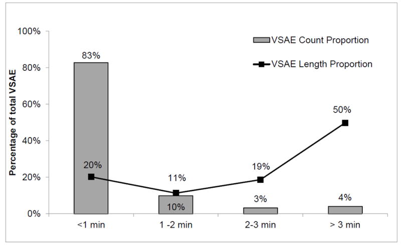
Proportion of vital sign alert events (VSAE) lasting >1 minute, 1 to 2 minutes, 2-3 minutes and >3 minutes, in terms of count and aggregated length, for both data sets combined for vitals other than BP, as described in the text.

Alert Annotation by Experts

Human annotation is time consuming and prone to bias. To increase annotation reliability and efficiency, we used an active ML based annotation framework. As shown in Panel A of Supplemental Digital Content 3, two reviewers first independently scored alerts presented as time series plots (Supplemental Digital Content 4) as real (+) or artifact (-) on a +3 to -3 scale, with +3 as certain real, 0 as unable to classify, and -3 as certain artifact. A combined score of ≥4 or ≤-4 from a reviewer pair were agreements (Panel B in Supplemental Digital Content 3). Pair scores between +3 and -3 required a third reviewer. If the cumulative three-reviewer score was ≥6 or ≤-6, it was included in the training set. Otherwise, that example was presented to the 4-member committee in a face-to-face meeting, reviewed, discussed, and re-adjudicated by majority vote. If committee consensus could not be reached for a given epoch, it was not used for training (26,27). The kappa coefficient for the paired review was positive when they were in agreement (0.28±0.05 and 0.29±0.03) and negative when they were not (-0.23±0.05 and -0.15±0.01) for BP and SpO₂ respectively. For epochs with disagreement after full committee re-adjudication, the kappa coefficient increased to 0.34±0.03 and 0.23±0.008 respectively, suggesting our adjudication process improved the agreement amongst expert reviewers. Although these may seem low levels of agreement, they underscore the lack of validity of single expert scoring systems of many such categorization processes presently being reported.

The selection for each batch was informed by an active learning algorithm called “Active Regression for Informative Projection Retrieval (Active RIPR)” (28). Initial batch selections were random samples. For subsequent batches, Active RIPR relearned the model from all previously annotated examples and determined the next most useful set of samples for annotation according to an information-gain criterion. This maximized the chance of developing an accurate model with minimum human effort. For the external test set, sample selection was based on a stratified sampling procedure so that samples were representative of the distribution of VS type in the population. The reviewer annotation process was implemented via a custom-developed web application (26,27,29). To annotate 973 alerts from training and test sets combined, we devoted about 100 hours of effort from each individual reviewer and about 15 hours in committee meetings.

Feature extraction

We extracted features from VSAE epochs with respect to signal sparsity, periodicity, or smoothness. Supplemental Digital Content 2 lists the complete set of features. We excluded features with missing values when used in algorithms that cannot handle missing data, while keeping the full set of features for algorithms that can handle missingness. We adopted a multivariate approach where features across all VS were used in models for each VS alert type. (i.e. HR, RR, SpO₂ and BP features were all used to model RR alerts etc.)

Offline model derivation and selection using 3-minute epochs

In the first experiment, we derived offline classification models for multiple ML algorithms using features from alert start until 3 minutes into the epoch (Figure 2A). ML algorithms used were: K nearest neighbors (KNN, at various K), Naïve Bayesian classifier (NB), Logistic Regression (LR), Support Vector Machine (SVM), and Random Forest (RF) (17-19). For each VS alert type, we identified best-performing models based on their 10-fold cross-validated Area under the Receiver (AUC) scores from the training/validation set. We also evaluated performance by applying models to the held-out test set. Too few HR artifacts were available to reliably learn a model for HR alerts.

Figure 2.

Timeframes of the first experiment (Panel A) for offline classification of alerts, and for the second experiment (Panel B) for online classification as the vital sign alert events (VSAE) evolve.

A. In Experiment 1, which classifies alerts as either real or artifact offline, only the initial period of VSAE is considered: from the time the vital sign first exceeds the threshold of abnormality, until 3 minutes into the event.

B. In the Experiment 2, which classifies alerts as either real or artifact online (as they evolve), a sequence of 3 minute windows is considered. The first of these windows ends at the start of VSAE, the last of them ends at 3 minute mark into VSAE, and the sequence is spaced at 20 second intervals.

Online artifact classification

In the second experiment, we evaluated the system’s online adjudication performance. For each alert we constructed a series of moving windows (Figure 2B) 3 minutes wide (180s), each ending at 0, 20, 40 seconds and so on up to the 180 second timestamp from the alert start. We applied the best performing classifier learned from the 3-minute VSAE epoch (detailed in the first experiment) to this set of consecutive windows to yield a series of prediction scores between 0 and 1 (the higher the score, the higher the likelihood of the alert to be real and vice versa). We summarized the trend of AUC scores and the predicted probability of real alerts over time.

RESULTS

Table 1 summarizes the baseline data for the training/validation and test sets. Offline results from the first experiment are detailed in the Supplemental Digital Content 1. In summary, the RF model showed consistently good performance across all three VS types, with 10-fold cross validation AUC scores in the training/validation set at 0.88 (95%CI 0.85-0.90) for BP, 1.0 (95% CI 1.0-1.0) for RR, and 0.89 (95%CI 0.88-0.910) for SpO₂. Performance on the external test set degraded slightly but remained robust (BP AUC 0.87 [95% CI 0.68-0.95], RR 0.97 [95% CI 0.93-1.0], SpO₂ 0.87 [95% CI 0.72-0.95]).

Online results from the second experiment are displayed in Figures 3 and 4. In Figure 3, the AUC score temporal trends for both the training/validation and external test sets demonstrate scores significantly better than random, even when the VS first crossed threshold. Discriminative power increased as time evolved. The performance on the test set shows that the BP AUC started at 0.77 and improved to 0.87 (0 to 180s window) while for RR, the first window’s AUC was 0.85, and for SpO₂ was 0.79.

Figure 3.

Area Under the Receiver Operating Charcteristic Curve (AUC) scores charted for each of the time windows for time elapsed since alert start (i.e. since a vital sign (VS)crossed its threshold). Results for the 3 minute window ending at the alert start correspond to the time of 0 seconds in the graphs. Results for the window ending 180 seconds into the alert corrrespond 180s time marks. Panel A shows the scores from 10-fold cross validation on the training/validation set; the shaded bands represent the 95%-ile bootstrap confidence intervals computed using 1,000 random splits of training/validation data. Panel B shows the results on the external test set given the model learned from the 3-minute epochs of training/validation data; the shaded bands represents the 95%-ile bootrstrap confidence intervals computed using 1,000 draws of the held-out test data. For all three VS, artifacts were well discriminated from real alerts event at the alert start, suggesting that artifact and real alerts are discernible even in advance of the the VS reaching the threshhold of instability. Respiratory rate (RR) shows a more progressive trend in which the discrimiative power increases further from about 1.5 minutes into the alert, as compared to milder trends dispayed for blood pressure (BP) and pulse oximetry (SpO₂).

A. Online performance observed using 10-fold cross validation on train/validation set

B. Online performance observed with the external test set

Figure 4.

Average prediction scores for groups of alerts annotated as real (solid line) and as artifacts (dotted line), charted along the time axis with respect to the alert time elapsed, obtained from the external test set using the model trained on training/validation set. The gray bands show 95%-ile confidence intervals. Discernability of true alerts vs. artifact increases as more vital sign information is collected over duration of vital sign alert event (VSAE) episodes.

Key: HR=heart rate, RR=respiratory rate, SpO₂=pulse oximetry, BP=blood pressure.

Figure 4 shows temporal trends of model’s average prediction scores by VS type for real alerts (solid line) or artifact (dotted line) from test set results. Across all VS types, the prediction scores for real alerts and artifact were well separated, with separation being most obvious for RR and least obvious but still clear for SpO₂. Among real alerts, the average prediction score showed a non-decreasing trend with various degrees of uncertainty, with RR relatively stable at high values, while BP and SpO₂ trends were somewhat milder and with larger variance. Among artifacts, the trend of the prediction score was downwards for all three VS types (RR showed the most prominent downward trend), suggesting that the two alert classes become more distinguishable as the alert progresses.

We next assessed the real and artifact discrimination in short duration alerts lasting less than 3 minutes. We selected 250 stratified samples from the external test set for each VS type (HR, RR and SpO₂) with time lengths falling into one of three bins (<1 min, 1-1.999 min, 2 to 2.999 min) which were annotated following the same procedure described. 72%, 16% and 5% of SpO₂, RR and HR alerts respectively were annotated as artifact. We applied the model learned from the 3-minute epochs to these short alerts for SpO₂ and RR only (no models were developed for HR due to its low artifact prevalence, while noninvasive BP cycling frequency did not conform to short alert periods). The overall AUC for offline discrimination was 0.82 (95% CI 0.69-0.91) for RR and 0.85 (95% CI 0.72-0.94) for SpO₂, while discrimination for online performance at timestamp 0, 20 and up to 120 seconds ranged from 0.83-0.97 for RR, and 0.88-0.95 for SpO₂.

If we threshold the output of the classifier so that the chance of misclassifying a real alert as artifact is 30%, we can correctly identify 92% and 88% of RR and SpO₂ artifact alarms respectively, combining both long and short duration alerts. This would translate to an overall alert reduction rate of about 30% after taking into account the artifacts prevalence in the data.

DISCUSSION

This study has five interesting findings, all of which have clinical implications for non-invasive monitoring strategies. First, using a defined workflow for consensus-driven annotation by a group of experts, as well as using algorithm-guided sample selection, resulted in better annotation agreement and improved efficiency. Our approach may have application in other ML studies wherein ground truth is ambiguous and subjective.

Second, as persistence requirements of alert duration increased, the total number of alerts markedly decreased. Duration of <1 minute constituted 83% of VSAE counts but only 20% of aggregate alert time, while duration of >3 minutes accounted for 4% of VSAE counts but 50% of aggregate alert time. Some literature suggests that one option to decrease alarm fatigue may be to increase persistence requirements to screen out short duration alerts (13,15,30). However, a large proportion of our single-parameter VS alerts <3 minutes represented true instability. Therefore, applying persistence screens alone may suppress real alerts of instability in its early stages of evolution, and miss important cues to future persistent instability and opportunity to intervene. In some SDU patients, cardiorespiratory reserve may be conserved and a longer persistence tolerated, while in less resilient patients even a short persistence may represent important physiologic compromise. As we show here and have others, the features between alerts due to real instability and artifact are inherently different (31, 32). It therefore becomes more attractive to develop smarter discriminative alarms by recognizing these feature differences, rather than simply dismissing short alerts. The methods we propose may provide a practical implementation of this technology (33).

Third, when ML algorithms developed in the training/validation set were evaluated on unseen test-set data, they remained robust. Although the two data sets were from the same clinical unit, they were temporally separate from each other, with different patients and clinicians cycling though over the study timeframe. Thus, the ML algorithms identified fundamental patterns inherent in the fundamental aspects of instability and not in the act of monitoring itself.

Fourth, our approach showed good discrimination between real instability or artifact even when the VS alert threshold is just crossed. When run in real time, BP slightly improved its performance, while RR and SpO₂ were both consistent in identifying real alerts early, but identified artifact with markedly better precision as the alerts evolved. Figure 4 shows that the average true alert prediction scores show non-decreasing tendency over the alert duration, while the same scores predicted for the artifacts consistently decreased with the largest drop noted for RR artifacts. The difference in the prediction uncertainty between the true alert and artifact test cases suggests that real alerts are generally more homogeneous when compared to the diverse reasons causing artifact.

Finally, the proportion of real to artifact alerts were slightly different when extending the alert window from very short (<3 min) to longer (≥3 min) event durations, with RR alerts being more likely artifact with immediate alerts and SpO₂ with prolonged events. Still, the algorithms identified each with a comparable degree of fidelity.

Limitations

Supervised ML needs reliable annotations to create robust predictive models. Our “ground truth” definition of alerts as real or artifact was defined by an expert committee, who may have applied an incorrect label. Nevertheless, the process of annotation by committee, supported by active learning selection of the most informative cases, appears to be more robust than annotation by only one or two experts. Furthermore, if alerts were ambiguous, they were censored so as to not contaminate the training data set. Second, for some VS, the prevalence of artifacts was rare compared to real alerts, as in the case for HR alerts. Our requirements for tolerance and persistence of the annotated VSAE epochs may have screened out artifacts, losing key discriminatory information and blunting the models. However, model performance was still robust when applied to short duration alerts, suggesting that both short and longer alerts can be discriminated using similar features. Finally, some minor disparity between the training/validation and test sets alert prevalence and VS type may have contributed to novel features in the test set, although this would bias results to be weaker than they could have been otherwise. Although there is no a priori reason to believe our approach would not generalize to data acquired in other centers via different monitoring platforms, the possibility exists that the algorithm performance could deteriorate if implemented “as is” on such systems.

CONCLUSIONS

Bedside instability recognition is impaired by lack of discrimination between real alerts and artifact (34, 35). Using multivariate VS features, ML algorithms can discriminate between real alerts and artifact as alerts evolve in real time. When further refined, they have potential to enable differential alarm recognition and clinical action. While “alarm hazards” remain at or near the top ten technology safety concerns (36,37), it is vital that mechanisms to improve monitoring safety are undertaken. Approaches such as the one we developed are certainly within reach of existing monitoring platforms and would take the form of software upgrades or extensions.

References

- 1.Otero A, Félix P, Barro S, Palacios F. Addressing the flaws of current critical alarms: a fuzzy constraint satisfaction approach. Artif Intell Med. 2009;47:219–238. doi: 10.1016/j.artmed.2009.08.002. [DOI] [PubMed] [Google Scholar]
- 2.Takla G, Petre JH, Doyle DJ, Horibe M, Gopakumaran B. The problem of artifacts in patient monitor data during surgery: a clinical and methodological review. Anest Analg. 2006;103:1196–1204. doi: 10.1213/01.ane.0000247964.47706.5d. [DOI] [PubMed] [Google Scholar]
- 3.Smith M. Rx for ECG monitoring artifact. Crit Care Nurse. 1984;4:64. [PubMed] [Google Scholar]
- 4.Boumbarov O, Velchev Y, Sokolov S. ECG personal identification in subspaces using radial basis neural networks. Intelligent Data Acquisition and Advanced Computing Systems: Technology and Applications. 2009 IDAACS 2009 IEEE International Workshop on IEEE; 2009. pp. 446–451. [Google Scholar]
- 5.Paul JS, Reddy MR, Kumar VJ. A transform domain SVD filter for suppression of muscle noise artifacts in exercise ECG’s. IEEE Trans Biomed Eng. 2000;47:654–663. doi: 10.1109/10.841337. [DOI] [PubMed] [Google Scholar]
- 6.Marque C, Bisch C, Dantas R, Elayoubi S, Brosse V, Perot C. Adaptive filtering for ECG rejection from surface EMG recordings. J Electromyog Kinesiol. 2005;15:310–315. doi: 10.1016/j.jelekin.2004.10.001. [DOI] [PubMed] [Google Scholar]
- 7.Lu G, Brittain J-S, Holland P, et al. Removing ECG noise from surface EMG signals using adaptive filtering. Neurosci Lett. 2009;462:14–19. doi: 10.1016/j.neulet.2009.06.063. [DOI] [PubMed] [Google Scholar]
- 8.Browne M, Cutmore T. Adaptive wavelet filtering for analysis of event-related potentials from the electro-encephalogram. Med Biol Eng Comput. 2000;38:645–652. doi: 10.1007/BF02344870. [DOI] [PubMed] [Google Scholar]
- 9.Thakral A, Wallace J, Tomlin D, Seth N, Thakor NV. Medical Image Computing and Computer-Assisted Intervention–MICCAI 2001. Springer; 2001. Surgical motion adaptive robotic technology (SMART): Taking the motion out of physiological motion; pp. 317–325. [Google Scholar]
- 10.Siebig S, Kuhls S, Imhoff M, Gather U, Schölmerich J, Wrede CE. Intensive care unit alarms--How many do we need? Crit Care Med. 2010;38:451–456. doi: 10.1097/CCM.0b013e3181cb0888. [DOI] [PubMed] [Google Scholar]
- 11.Couceiro R, Carvalho P, Paiva R, Henriques J, Muehlsteff J. Detection of motion artifacts in photoplethysmographic signals based on time and period domain analysis. Conf Proc IEEE Eng Med Biol Soc 2012; 2012. pp. 2603–2606. [DOI] [PubMed] [Google Scholar]
- 12.Sendelbach S, Funk M. Alarm fatigue: a patient safety concern. AACN Adv Crit Care. 2013;24:378–386. doi: 10.1097/NCI.0b013e3182a903f9. [DOI] [PubMed] [Google Scholar]
- 13.Cvach M. Monitor alarm fatigue: an integrative review. Biomed Instrum Technol. 2012;46:268–277. doi: 10.2345/0899-8205-46.4.268. [DOI] [PubMed] [Google Scholar]
- 14.Blake N. The Effect of Alarm Fatigue on the Work Environment. AACN Adv Crit Care. 2014;25:18–19. doi: 10.1097/NCI.0000000000000009. [DOI] [PubMed] [Google Scholar]
- 15.Graham KC, Cvach M. Monitor alarm fatigue: standardizing use of physiological monitors and decreasing nuisance alarms. Am J Crit Care. 2010;19:28–34. doi: 10.4037/ajcc2010651. [DOI] [PubMed] [Google Scholar]
- 16.Gazarian PK. Nurses’ response to frequency and types of electrocardiography alarms in a non-critical care setting: A descriptive study. Int J Nurs Stud. 2014;51:190–197. doi: 10.1016/j.ijnurstu.2013.05.014. [DOI] [PubMed] [Google Scholar]
- 17.Kruppa J, Liu Y, Biau G, et al. Probability estimation with machine learning methods for dichotomous and multicategory outcome. Theory Biom J. 2014;56:534–563. doi: 10.1002/bimj.201300068. [DOI] [PubMed] [Google Scholar]
- 18.Mohri M, Rostamizadeh A, Talwalkar A. Foundations of machine learning. MIT press; 2012. [Google Scholar]
- 19.Bishop CM. Pattern recognition and machine learning. Springer; New York: 2006. [Google Scholar]
- 20.Acharya UR, Sree SV, Ribeiro R, et al. Data mining framework for fatty liver disease classification in ultrasound: A hybrid feature extraction paradigm. Med Phys. 2012;39:4255–2264. doi: 10.1118/1.4725759. [DOI] [PubMed] [Google Scholar]
- 21.Acharya UR, Sree SV, Muthu Rama Krishnan M, et al. Automated classification of patients with coronary artery disease using grayscale features from left ventricle echocardiographic images. Comput Methods Programs Biomed. 2013;112:624–632. doi: 10.1016/j.cmpb.2013.07.012. [DOI] [PubMed] [Google Scholar]
- 22.Suzuki K. Machine Learning in Computer-Aided Diagnosis of the Thorax and Colon in CT: A Survey. IEICE Trans Inf Syst. 2013;E96-D(4):772–783. doi: 10.1587/transinf.e96.d.772. [DOI] [PMC free article] [PubMed] [Google Scholar]
- 23.Halford JJ, Schalkoff RJ, Zhou J, et al. Standardized database development for EEG epileptiform transient detection: EEGnet scoring system and machine learning analysis. J Neurosci Methods. 2013;212:308–316. doi: 10.1016/j.jneumeth.2012.11.005. [DOI] [PubMed] [Google Scholar]
- 24.Kim S, Hamilton R, Pineles S, Bergsneider M, Hu X. Noninvasive Intracranial Hypertension Detection Utilizing Semisupervised Learning. Biomedical Engineering. IEEE Trans Biomed Eng. 2013;60:1126–1133. doi: 10.1109/TBME.2012.2227477. [DOI] [PMC free article] [PubMed] [Google Scholar]
- 25.Zweigenbaum P, Lavergne T, Grabar N, Hamon T, Rosset S, Grouin C. Combining an expert-Based Medical entity Recognizer to a Machine-Learning system: Methods and a case study. Biomed Inform Insights. 2013;6(Suppl 1):51–62. doi: 10.4137/BII.S11770. [DOI] [PMC free article] [PubMed] [Google Scholar]
- 26.Wang D, Chen L, Fiterau M, Dubrawski A, Hravnak M, Bose E, Wallace D, Kaynar M, Clermont G, Pinsky MR. Multi-tier ground truth elicitation framework with application to artifact classification for predicting patient instability. J Intensive Care Med. 2014;40(1 Suppl):S289. [Google Scholar]
- 27.Wang D, Fiterau M, Dubrawski A, Hravnak M, Clermont G, Pinsky MR. Interpretable active learning in support of clinical data annotation. Crit Care Med. 2014;42(12 Suppl):797. [Google Scholar]
- 28.Fiterau M, Dubrawski A. Active learning for Informative Projection Recovery. Conference of the Association for the Advancement of Artificial Intelligence; 2015. AAAI 2015. [Google Scholar]
- 29.Hravnak M, Chen L, Fiterau M, Dubrawski A, Clermont G, Guillame-Bert M, Bose E, Pinsky MR. Active machine learning to increase annotation efficiency in classifying vital sign events as artifact or real alerts in continuous noninvasive monitoring. Am J Resp and Crit Care Med. 2014 doi: 10.1164/ajrccm-conference.2014.189.1A3627. A3627. [DOI] [Google Scholar]
- 30.Dandoy CE, Davies SM, Flesch L, Hayward M, Doons C, Coleman K, Jacobs J, McKenna LA, Olomajeye A, Olson C, Powers J, Shoemaker K, Jodale S, Allassandrini E, Weiss B. A team-based approach to reducing cardiac monitor alarms. Pediatrics. 2014;134:e1686–e1694. doi: 10.1542/peds.2014-1162. [DOI] [PubMed] [Google Scholar]
- 31.Hravnak M, Chen L, Bose E, Fiterau M, Guillame-Bert M, Dubrawski A, Clermont G, Pinsky MR. Real alerts and artifact in continuous non-invasive vital sign monitoring: Mono-vs. Multi-process. Crit Care Med. 2013;41(Suppl 12):A66. [Google Scholar]
- 32.Fiterau M, Dubrawski A, Hravnak M, Chen L, Pinsky MR, Clermont G, Bose E. Archetyping artifacts in monitored noninvasive vital signs data. Crit Care Med. 2014;42(12 Suppl):51. [Google Scholar]
- 33.Funk M, Clark JT, Bauld TJ, Ott JC, Coss P. Attitudes and practices related to clinical alarms. Am J Crit Care. 2014;23:e9–e18. doi: 10.4037/ajcc2014315. [DOI] [PubMed] [Google Scholar]
- 34.Rayo MF, Moffatt-Bruce SD. Alarm system management: evidence-based guidance encouraging direct measurement of informativeness to improve alarm response. BMJ Qual Saf. 2015;24:282–286. doi: 10.1136/bmjqs-2014-003373. [DOI] [PubMed] [Google Scholar]
- 35.Hravnak M, DeVita MA, Clontz A, Edwards L, Valenta C, Pinsky MR. Cardiorespiratory instability before and after implementing an integrated monitoring system. Crit Care Med. 2011;39(1):65–72. doi: 10.1097/CCM.0b013e3181fb7b1c. [DOI] [PMC free article] [PubMed] [Google Scholar]
- 36.Drew BJ, Harris P, Zegre-Hensey JK, Mammone T, Schindler D, Salas-Boni R, Bai Y, Tinoco A, King Q, Hu X. Insights into the problem of alarm fatigue with physiologic monitoring devices: a comprehensive observational study of consecutive intensive care unit patients. PloS One. 2014 Oct 22;9(10):e110274. doi: 10.1371/journal.pone.0110274. eCollection 2014. [DOI] [PMC free article] [PubMed] [Google Scholar]
- 37.Keller JP., Jr Clinical alarm hazards: a “top ten” health technology safety concern. J Electrocardiol. 2012;45:588–91. doi: 10.1016/j.jelectrocard.2012.08.050. [DOI] [PubMed] [Google Scholar]
Associated Data
This section collects any data citations, data availability statements, or supplementary materials included in this article.