STGP: Spatio-Temporal Gaussian Process Models for Longitudinal Neuroimaging Data

Abstract

Longitudinal neuroimaging data plays an important role in mapping the neural developmental profile of major neuropsychiatric and neurodegenerative disorders and normal brain. The development of such developmental maps is critical for the prevention, diagnosis, and treatment of many brain-related diseases. The aim of this paper is to develop a spatio-temporal Gaussian process (STGP) framework to accurately delineate the developmental trajectories of brain structure and function, while achieving better prediction by explicitly incorporating the spatial and temporal features of longitudinal neuroimaging data. Our STGP integrates a functional principal component model (FPCA) and a partition parametric space-time covariance model to capture the medium-to-large and small-to-medium spatio-temporal dependence structures, respectively. We develop a three-stage efficient estimation procedure as well as a predictive method based on a kriging technique. Two key novelties of STGP are that it can efficiently use a small number of parameters to capture complex non-stationary and non-separable spatio-temporal dependence structures and that it can accurately predict spatio-temporal changes. We illustrate STGP using simulated data sets and two real data analyses including longitudinal positron emission tomography data from the Alzheimers Disease Neuroimaging Initiative (ADNI) and longitudinal lateral ventricle surface data from a longitudinal study of early brain development.

1 Introduction

Large-scale longitudinal neuroimaging studies have collected a rich set of ultra-high dimensional imaging data, behavioral data, and clinical data in order to better understand the progress of neuropsychiatric disorders, neurological disorders and stroke, and normal brain development, among many others [Evans and Group., 2006, Almli et al., 2007, Skup et al., 2011, Meltzer et al., 2009, Kim et al., 2010, Weiner et al., 2013]. Three primary goals of longitudinal neuroimaging studies are

• (i) to characterize individual change in brain structure and function over time;

• (ii) to characterize the effect of some covariates of interest, such as diagnostic status and gender, on the individual change; and

• (iii) to study the predictive value of early brain developmental trajectories for later brain and cognitive development and disease progression.

Moreover, the objective 2 of the recent National Institute of Mental Health (NIMH) Strategic Plan is to chart mental illness trajectories to determine when, where, and how to intervene by using novel techniques (e.g., imaging). To achieve these goals (i)-(iii), it requires the development of advanced image processing and statistical tools.

A distinctive feature of longitudinal neuroimaging data is that it contains both spatial and temporal dimensions. Specifically, imaging measurements of the same individual usually exhibit positive correlation and the strength of the correlation decreases with the time separation. Moreover, due to the inherent biological structure and function of brain, neuroimaging data are spatially correlated in nature and contain spatially contiguous regions. However, since longitudinal neuroimaging data usually has strong heterogeneity in longitudinal trajectories across space, their spatial and temporal dimensions are typically non-separable. Such non-separability has posed unprecedented challenges to most existing statistical methods for achieving goals (i)-(iii). As shown in Derado et al. [2010], appropriately accounting for correlation structure in statistical modeling and estimation can lead to substantial gains in statistical power. Furthermore, accurately modeling the spatial and temporal dependencies is even more critical for prediction [Cressie and Wikle, 2011, Derado et al., 2013, Demel and Du, 2015].

There are two major groups of spatio-temporal models for longitudinal neuroimaging data. The first one is to use temporal evolution models for non-linear image registration to estimate longitudinal spatial transformations that capture time-varying images [Ashburner and Ridgway, 2012, Singh et al., 2015, Hong et al., 2012]. Such temporal evolution models are usually characterized by some regularizing term and identified either by fitting parametric progression models on geometric features of the transformation or by choosing an opportune metric in the space of transformations to characterize specific evolution models in the image space. These models usually cannot capture complex spatial-temporal correlation of longitudinal neuroimaging data. The second one, usually identified as voxel-based analysis, is to fit some parametric or semi-parametric regression models (e.g., linear mixed effects and estimating equations) at each voxel of registered images [Bernal-Rusiel et al., 2013, Li et al., 2013, Yuan et al., 2013, Guillaume et al., 2014, Skup et al., 2012]. These models usually ignore the moderate-to-long range spatial correlation of imaging data, even though local spatial correlation is usually introduced by the use of Gaussian smoothing with some apriori kernel size.

Recently, there is a growing interest in modeling complex spatial-temporal correlation of longitudinal neuroimaging data [Marco et al., 2015, Lorenzi et al., 2015, Derado et al., 2013, Guo et al., 2008, Woolrich et al., 2004, Gössl et al., 2001, Brezger et al., 2007, Penny et al., 2005]. Such models are important for using longitudinal neuroimaging to guide treatment selection for individual patients and predict the progression of disease. For instance, in Guo et al. [2008], a predictive statistical model for PET and fMRI data was proposed to forecast a patient's brain activity following a specified treatment regimen. In Derado et al. [2013], a Bayesian spatial hierarchical model was proposed for predicting follow-up neural activity based on an individual's baseline functional neuroimaging data. In Marco et al. [2015] and Lorenzi et al. [2015], two novel spatio-temporal generative models were proposed by using either the Kronecker product of spatial and temporal covariance matrices or the kernel convolutions of a white noise Gaussian process. In general, borrowing strength from the spatial correlations as well as capturing temporal correlations between brain activity can significantly improve predictive performance.

The aim of this paper is to develop a spatio-temporal Gaussian process (STGP) framework to efficiently and flexibly model the spatial and temporal correlation structure of longitudinal neuroimaging data. Compared with the existing literature [Marco et al., 2015, Lorenzi et al., 2015, Derado et al., 2013, Guo et al., 2008, Woolrich et al., 2004, Gössl et al., 2001, Brezger et al., 2007, Penny et al., 2005], we make several novel contributions. (i) Our STGP uses a functional principal component model (FPCA) to capture a large portion of spatio-temporal dependence structure, while it uses a partition space-time covariance model to capture some local spatio-temporal correlations. In particular, the basis functions for FPCA are directly learnt from data and can capture some key features of longitudinal neuroimaging data, which may not be easily modeled by using specific parametric models (e.g., Markov random field). In contrast, most existing models either assume some specific parametric models (e.g., autoregressive and Markov random field) or use the kernel convolutions of a white noise Gaussian process for a fixed kernel function. (ii) We develop a three-stage efficient estimation procedure to estimate all parameters associated with the spatio-temporal dependence structure. (iii) We propose a prediction method that borrows strength from the spatial and temporal correlations to achieve much better prediction of spatio-temporal changes. (iv) We use two real data sets to illustrate that STGP is a powerful tool for quantifying and/or predicting the spatio-temporal changes of brain structure and function. A more general software package is under development and will be made publicly available at the URL http://www.bios.unc.edu/research/bias/software.html.

2 Methods

2.1 Model formulation

Consider a longitudinal neuroimaging study with n subjects. We observe neuroimaging measures (e.g., cortical thickness), denoted by {y_i(d, t_ij)}, at voxel d of a three-dimensional (3D) volume (or 2D surface), denoted by 𝒟, and a p×1 vector of covariates (e.g., age, gender, and diagnostic status), denoted by x_i(t_ij) = (x_i,1 (t_ij), …, x_i,p (t_ij))^T, for the i–th subject at time t_ij ∈ 𝒯 for i = 1, …, n and j = 1, …, m_i, where m_i denotes the total number of time points for the i-th subject. Without loss of generality, 𝒟 and 𝒯 are assumed to be compact sets in ℝ³ and ℝ, respectively, and N_D denotes the number of voxels in 𝒟.

The measurement model of our spatio-temporal Gaussian process (STGP) is given by

$$y_i(d,t)=\mu (d,{\mathbf{x}}_i(t))+{\eta }_i(d,t)+{\epsilon }_i(d,t)\text{for}i=1,\dots ,n,$$ (1)

where μ(d, x_i(t)) is the mean structure for characterizing the effects of covariates x_i(t) = (x_i,1(t), …, x_i,p(t))^T on longitudinal neuroimaging data across (d,t). The η_i(d,t) are random functions that characterize both individual image variations from μ(d, x_i(t)) and the medium-to-long-range dependence of longitudinal imaging data. Moreover, ε_i(d, t) are measurement errors that capture the local spatio-temporal dependence structure of longitudinal imaging data. It is assumed that η_i(d,t) and ε_i(d,t) are mutually independent and η_i(d,t) and ε_i(d,t) are, respectively, independent and identical copies of GP(0, Σ_η) and GP(0, Σ_ε), where GP(μ, Σ) denotes a Gaussian process with mean function μ(d, t) and covariance function Σ((d, t), (d′, t′)).

We consider a functional principal component analysis (FPCA) model for the process η_i(d, t) or a spectral decomposition of Σ_η((d, t), (d′, t′)). Let λ₁ ≥ λ₂ ≥ … ≥ 0 be the ordered eigenvalues of the linear operator determined by Σ_η with ${\sum }_{l=1}^{\infty }{\lambda }_l<\infty$ and the ψ_l(d,t)'s be the corresponding orthonormal eigenfunctions [Yao and Lee, 2006, Hall et al., 2006, Chiou et al., 2004]. Then the spectral decomposition of Σ_η((d, t), (d′, t′)) is given by

$${\sum }_{\eta }((d,t),(d^{\prime },t^{\prime }))=\sum _{l=1}^{\infty }{\lambda }_l{\psi }_l(d,t){\psi }_l(d^{\prime },t^{\prime }).$$ (2)

Then η_i(d,t) admits the Karhunen-Loeve expansion as follows:

$${\eta }_i(d,t)=\sum _{l=1}^{\infty }{\xi }_{i,l}{\psi }_l(d,t),$$ (3)

where ξ_i,l = ∫_𝒯 ∫_d∈𝒟 η_i(d,t)ψ_l(d,t)d𝒱(d)dt is referred to as the l-th functional principal component score of the i-th subject, in which d𝒱(s) denotes the Lebesgue measure. The ξ_i,l's are uncorrelated random variables with E(ξ_i,l) = 0 and $\mathrm{E}({\xi }_{i,l}^2)={\lambda }_l$. If λ_l ≈ 0 for l ≥ L₀ + 1, then (3) can be approximated by

$${\eta }_i(d,t)\approx \sum _{l=1}^{L_0}{\xi }_{i,l}{\psi }_l(d,t).$$ (4)

Compared with Lorenzi et al. [2015], a key advantage of using FPCA is that ψ_l(d,t) are directly estimated from the data.

To accurately characterize Σ_ε, we consider a partition covariance model for the local spatio-temporal dependence structure of imaging data. Specifically, we partition 𝒟 into K mutually exclusive brain regions of interest, denoted as {C_k : k = 1, …, K}, and then fit a parametric spatio-temporal model for each C_k. Moreover, ε_i(d,t) are assumed to be independent across partitioned brain regions, while the spatial-temporal correlation is preserved within each subregion. If we set K to be 1, then it reduces to the use of a single parametric model to fit residuals across all voxels in 𝒟. When K is relatively large, the partition covariance model can dramatically increase flexibility and robustness in capturing local correlations.

There are at least two approaches for determining exclusive brain regions of interest. The first one is to use some existing anatomical parcellations of brain regions [Derado et al., 2013]. A major drawback is that residuals ε_i(d,t) within each of these pre-defined regions may not be spatially correlated. Instead, we use the second approach based on a Gaussian mixture model to cluster 𝒟 into K homogeneous regions. We will describe such mixture model in Section 2.2.

We add a subscript k(d) to denote the functional cluster to which voxel d belongs. Finally, for the k–th region of interest, we obtain an approximation of model (1) given by

$$y_{i,k(d)}(d,t)\approx \mu (d,{\mathbf{x}}_i(t))+\sum _{l=1}^{L_0}{\xi }_{i,l}{\psi }_l(d,t)+{\epsilon }_{i,k(d)}(d,t),$$ (5)

where ε_i,k(d)(d,t) satisfies

$$\text{Cov}({\epsilon }_{i,k(d)}(d,t),{\epsilon }_{i,k(d^{\prime })}(d^{\prime },t^{\prime }))=\{\begin{array}{cc}{\sum }_{\epsilon }((d,t),(d^{\prime },t^{\prime });{\mathit{\theta }}_k)& \text{if}k(d)=k(d^{\prime }),\\ 0& \text{otherwise},\end{array}$$ (6)

in which θ_k is a vector of unknown parameters in Σ_ε((d, t), (d′, t′);θ_k). If the observation indices are rearranged such that the observations within a cluster are grouped together, the covariance matrix Σ_ε = (Σ_ε((d, t), (d′, t′))) is block-diagonal.

2.2 Estimation procedure

We develop a three-stage estimation procedure as follows.

• Stage (I): Estimate the parametric (or nonparametric) regression function μ(·, ·).

• Stage (II): Estimate the covariance function Σ_η((d, t), (d′, t′)) and its associated eigenvalues and eigenfunctions.

• Stage (III): Estimate the unknown parameters in the partition covariance model by using a restricted maximum likelihood estimation.

Stage (I) is to estimate the mean function μ(d, x_i(t)) at voxel d by pooling the data from all subjects. There is a large literature on the estimation of μ(d, x_i(t)). We need to distinguish two scenarios. The first one is the dense sampling design, in that the number of observations per subject is relatively larger, that is, min_i m_i → ∞. It often assumes that μ(d, x_i(t)) is a nonparametric function of x_i(t). In this case, we need to resort to some nonparametric methods (e.g., penalized spline or local polynomial) to approximate μ(d, x_i(t))[Yao and Lee, 2006, Ruppert et al., 2003, Fan and Gijbels, 1996]. The second one is the sparse sampling design, in that the number of observations per subject is relatively small, that is, max_i m_i < ∞. In this case, we may consider a parametric function of μ(d, x_i(t)) based on either linear (or nonlinear) mixed effects models or generalized estimating equations μ(d, x_i(t)) [Bernal-Rusiel et al., 2013, Li et al., 2013, Guillaume et al., 2014, Skup et al., 2012]. Moreover, even under this scenario, if time points t_ij are randomly drawn, we may fit a nonparametric function of μ(d, x_i(t)).

Stage (II) is to estimate Σ_η(·, ·) and its eigenvalues and eigenfunctions. Stage (II) consists of three steps as follows.

• Step (II.1) is to calculate all individual functions η_i(d,t) using nonparametric regression techniques. For the dense sampling design, we apply a local linear regression method to smooth r_i(d,t) = y_i(d,t) − μ̂(d, x_i(t)) over (d,t). Let $K_h(d_m-d)=h^{-3}{\prod }_{j=1}^{3}K((d_{m,j}-d_j)/h)$ be the rescaled kernel function with a bandwidth h, where K(·) is a univariate kernel function. For each i, we estimate η_i(d,t) by minimizing

  $$\sum _{m=1}^{N_D}\sum _{j=1}^{m_i}{\{r_i(d_m,t_{ij})-{\beta }_0-{\mathit{\beta }}_1^T{({(d_m-d)}^T,t_{ij}-t)}^T\}}^2{K}_h(d_m-d)K_{h_1}(t_{ij}-t)$$ (7)

  with respect to β₀ and β_l, where K_h1 (t_ij − t) = K((t_ij − t)/h₁)/h₁. The local linear estimator of η_i(d,t), denoted as η̂_i(d,t), is given by β̂₀. We pool the data from all n subjects, and the optimal bandwidth (h, h₁) is selected by minimizing the generalized cross-validation (GCV) score.

  However, for the sparse sampling design, we use the local linear regression method to smooth r_i(d,t) = y_i(d,t) − μ̂(d, x_i(t)) over d ∈ 𝒟 at each time point t_ij, which leads to a local linear estimator of η_i(d,t_ij), denoted as η̃_i(d,t_ij). Then, at each voxel, we pool out all observations {η̃_i(d,t_ij) : i = 1, …, n; j = 1, …, m_i} to estimate η_i(d,t) by using a random effects model given by

  $${\stackrel{\sim }{\eta }}_i(d,t)={\mathbf{z}}_i{(t)}^T{\mathit{\gamma }}_i(d)+{\delta }_i(d,t),$$ (8)

  where z_i(t) is a p_z × 1 vector of components that depends on time and/or some covariates, γ_i(d) is a p_z × 1 vector of random effects, and δ_i(d,t) are measurement errors. It is also assumed that γ_i(d) and δ_i(d,t) are independent and follow N(0, Σ_γ(d)) and $N(0,{\sigma }_{\delta }^2(d))$, respectively. For instance, we may set z_i(t) as (1, t, t²)^T or a vector of spline basis functions. We can estimate Σ_γ(d) and ${\sigma }_{\delta }^2(d)$ by using restricted maximum likelihood estimation and then calculate a prediction of γ_i(d), denoted as ${\widehat{\gamma }}_i(d)={\widehat{\sum }}_{\gamma }(d){\mathbf{z}}_i^T{\widehat{\sum }}_{{\eta }_i}{(d)}^{-1}{\stackrel{\sim }{\mathit{\eta }}}_i(d)$, where z_i = (z_i(t_i1), …, z_i(t_imi))^T, ${\widehat{\sum }}_{{\eta }_i}(d)={\mathbf{z}}_i{\widehat{\sum }}_{\gamma }(d){\mathbf{z}}_i^T+{\widehat{\sigma }}_{\delta }^2(d)I_{m_i}$, and η̃_i(d) = (η̃_i(d,t_i1), …, η̃_i(d,t_imi))^T. Finally, we set η̂_i(d, t) = z_i(t)^T γ̂_i(d) across (d, t).

• Step (II.2) is to estimate Σ_η((d, t), (d′, t′)) by using the empirical covariance matrix of η̂_i(d,t) as follows:

  $${\widehat{\sum }}_{\eta }((d,t),(d^{\prime },t^{\prime }))=n^{-1}\sum _{i=1}^n{\widehat{\eta }}_i(d,t){\widehat{\eta }}_i(d^{\prime },t^{\prime }).$$ (9)

  Then, we can use the singular value decomposition of (9) to estimate the eigenvalue-eigenfunction pairs of Σ_η((d,t), (d′, t′)) in (2). Let (t₁, …, t_NT)^T be an N_T × 1 vector of evenly spaced (or distributed) grid points in an interval [min_i,j(t_ij), max_i,j(t_ij)] such that t₁ = min_i,j(t_ij) < t₂ < … < t_NT = max_i,j(t_ij). Let η̂_i(t) = (η̂_i(d₁, t),…, η̂_i(d_ND, t))^T and η̂_i = (η̂_i(t₁)^T, …, η̂_i(t_NT)^T)^T be an N_D × 1 vector and an N_DN_T × 1 vector, respectively. Then, we have an N_DN_T × n matrix V = [η̂₁, …, η̂_n]. Since n is much smaller than N_DN_T, it is easier to calculate the eigenvalue-eigenvector pairs of the n × n matrix V^TV, denoted by {(λ̂_i, ψ̂_i) : i = 1, …, n}. It can be shown that {(λ̂_i, Vψ̂_i) : i = 1, …, n} are the eigenvalue-eigenvector pairs of the N_DN_T × N_DN_T matrix VV^T. It is common to choose a value L₀ in (4) based on the proportion of explained variance [Greven et al., 2010]. We chose the number of principal components so that the proportion of the cumulative eigenvalue is above a prefixed threshold.

• Step (II.3) is to compute the functional principal component scores ξ_i,l. it follows from (3) that estimating ξ̂_i,l is equivalent to solving a linear model given by

  $${\widehat{\eta }}_i(d,t)\approx \sum _{l=1}^{L_0}{\xi }_{i,l}{\widehat{\psi }}_l(d,t).$$

  Let ψ̂_l(t) = (ψ̂_l(d₁, t), …, ψ̂_l(d_ND, t))^T and ψ̂_il = (ψ̂_l(t_i1)^T, …, ψ̂_l(t_imi)^T)^T, respectively, be an N_D × 1 vector and an m_iN_D × 1 vector of the estimated l-th eigenfunction. Then, we have an m_iN_D × L₀ matrix Ψ̂_i = [ψ̂_i1, …, ψ̂_iL0]. We consider an estimate of the functional principal component score for the i-th subject as follows:

  $${\widehat{\mathit{\xi }}}_i={({\widehat{\xi }}_{i,1},\dots ,{\widehat{\xi }}_{i,L_0})}^T={({\widehat{\mathbf{\Psi }}}_i^T{\widehat{\mathbf{\Psi }}}_i)}^{-1}{\widehat{\mathbf{\Psi }}}_i^T{({\widehat{\mathit{\eta }}}_i{(t_{i1})}^T,\dots ,{\widehat{\mathit{\eta }}}_i{(t_{i{m}_i})}^T)}^T.$$ (10)

Stage (III) is to estimate all parameters in the partition covariance model as follows. We can estimate ε_i(d,t_ij) by using ${\widehat{\epsilon }}_i(d,t_{ij})=y_i(d,t_{ij})-\widehat{\mu }(d,{\mathbf{x}}_i(t_{ij}))-{\sum }_{l=1}^{L_0}{\widehat{\xi }}_{i,l}{\widehat{\psi }}_l(d,t_{ij})$ and concatenate them into a vector ε̂(d) = (ε̂_i(d, t_ij) : i = 1, …, n; j = 1, …, m_i)^T for each voxel. Specifically, we use a penalized likelihood approach with an L₁ penalty function for a Gaussian mixture model to cluster all residual vectors {ε̂(d) : d ∈ 𝒟} into K homogeneous regions [Pan and Shen, 2007, Huang et al., 2015].

Let ε̂_i,k(t) = (ε̂_i,k(d)(d,t) : d ∈ C_k) be a |C_k| × 1 vector for k = 1, …, K. Then we can write an m_i|C_k| × 1 vector ε̂_i,k = (ε̂_i,k(t_i1)^T, …, ε̂_i,k(t_imi)^T)^T and an m_iN_D × 1 vector ε̂_i = (ε̂_i,k : k = 1, …, K). We also define $\widehat{\mathit{\epsilon }}={({\widehat{\mathit{\epsilon }}}_1^T,\dots ,{\widehat{\mathit{\epsilon }}}_n^T)}^T$ and $\mathit{\theta }={({\mathit{\theta }}_1^T,\dots ,{\mathit{\theta }}_K^T)}^T$. Second, we calculate a restricted maximum likelihood (REML) estimate of θ by maximizing the REML log-likelihood given by

$$L(\mathit{\theta }|\widehat{\mathit{\epsilon }})=-\frac{1}{2}\sum _{i=1}^n\sum _{k=1}^{K}log|{\sum }_{i,\epsilon }({\mathit{\theta }}_k)|-\frac{1}{2}\sum _{k=1}^{K}log(\sum _{i=1}^n{\mathbf{1}}_{m_i|C_k|}^T{\sum }_{i,\epsilon }{({\mathit{\theta }}_k)}^{-1}{\mathbf{1}}_{m_i|C_k|})-\frac{1}{2}\sum _{i=1}^n\sum _{k=1}^K{({\widehat{\mathit{\epsilon }}}_{i,k}-{\mathbf{1}}_{m_i|C_k|}\widehat{\mathit{\mu }}({\mathit{\theta }}_k))}^T{\sum }_{i,\epsilon }{({\mathit{\theta }}_k)}^{-1}({\widehat{\mathit{\epsilon }}}_{i,k}-{\mathbf{1}}_{m_i|C_k|}\widehat{\mathit{\mu }}({\mathit{\theta }}_k)),$$ (11)

where Σ_i,ε(θ_k) is an m_i|C_k| × m_i|C_k| covariance matrix of ε_i,k = (ε_i,k(t_i1)^T, …, ε_i,k(t_imi)^T)^T, where ε_i,k(t) = (ε_i,k(d)(d,t) : d ∈ C_k), and 1_mi|Ck| is an m_i|C_k| × 1 vector having all the entries 1. Furthermore, μ̂(θ_k) is given by

$$\widehat{\mathit{\mu }}({\mathit{\theta }}_k)={(\sum _{i=1}^n{\mathbf{1}}_{m_i|C_k|}^T{\sum }_{i,\epsilon }{({\mathit{\theta }}_k)}^{-1}{\mathbf{1}}_{m_i|C_k|})}^{-1}\sum _{i=1}^n{\mathbf{1}}_{m_i|C_k|}^T{\sum }_{i,\epsilon }{({\mathit{\theta }}_k)}^{-1}{\widehat{\mathit{\epsilon }}}_{i,k}.$$

2.3 Prediction procedure

We present a prediction procedure based on a kriging technique. We start with splitting the data set into a training set and a test set. We fit the proposed model to the training set to estimate the fixed main effect, denoted as μ̂, eigenvalue-eigenfunction pairs, denoted as {(λ̂_l, ψ̂_l(d,t)) : l = 1, …, L₀}, and the parameters in the partition covariance model, denoted as θ̂. Then we use the prediction procedure given below to predict the image at time t₀ for the i₀-th subject in the test set, based on the images at time t_i0j ≠ t₀ and the fitted model.

Given μ̂ estimated from the training set, it is straightforward to calculate μ̂(d, x_i0(t)). Then we obtain r_i0(d, t_i0j) = y_i0(d,t_i0j)−μ̂(d, x_i0(t_i0j)). Given {(λ̂_l, ψ̂_l(d,t)) : l = 1, …, L₀}, we can follow Stage (II) in Section 2.2 to calculate {ξ̂_i0,_l : l = 1, …, L₀} for the i₀-th subject in the test set. Thus we can calculate

$${\widehat{\epsilon }}_{i_0,k(d)}(d,t_{i_{0}j})=y_{i_0,k(d)}(d,t_{i_{0}j})-\widehat{\mu }(d,{\mathbf{x}}_{i_0}(t_{i_{0}j}))-\sum _{l=1}^{L_0}{\widehat{\xi }}_{i_0,l}{\widehat{\psi }}_l(d,t_{i_{0}j})$$

across all voxels d at time t_i0j ≠ t₀. Then, we can use the spatio-temporal kriging to calculate ε̂_i0,k(d)(d, t₀) for all voxels d as follows. Let Σ_ε,k = Var(ε_i,k) and c_0,k = Cov(ε_i,k(t₀), ε_i,k). The kriging predictor is given by ε̂_i0,k(t₀) = c_0,k(Σ_ε,k)⁻¹ε̂_i0,k for k = 1, …, K. In practice, c_0,k and Σ_ε,k are estimated by plugging in the REML estimates, θ̂_k. Finally, we predict y_i0,k(d)(d,t₀) according to

$${\widehat{y}}_{i_0,k(d)}(d,t_0)=\widehat{\mu }(d,{\mathbf{x}}_{i_0}(t_0))+\sum _{l=1}^{L_0}{\widehat{\xi }}_{i_0,l}{\widehat{\psi }}_l(d,t_0)+{\widehat{\epsilon }}_{i_0,k(d)}(d,t_0)\text{for}d\epsilon \mathcal{D}.$$ (12)

2.4 Model validation

For each subject in the test set, we apply the prediction procedure described in Section 2.3 to predict the measurements across all voxels at time t_ij. We evaluate the prediction accuracy of STGP by quantifying the prediction error at each voxel d and time t_ij. Specifically, the square root of the mean squared prediction error (rtMSPE) for each voxel d is given by

$$\text{rtMSPE}(d)=\sqrt{\frac{1}{|{\mathcal{S}}_{\mathit{\text{TE}}}|}\sum _{i\in {\mathcal{S}}_{\mathit{\text{TE}}}}{({\widehat{y}}_{i,k(d)}(d,t_{ij})-y_{i,k(d)}(d,t_{ij}))}^2},$$ (13)

where 𝒮_TE denotes the index set of all the subjects in the test set and |𝒮_TE| is the cardinality of S_TE. The overall rtMSPE is calculated as follows:

$$\text{rtMSPE}=\sqrt{\frac{1}{|{\mathcal{S}}_{\mathit{\text{TE}}}|N_D}\sum _{i\in {\mathcal{S}}_{\mathit{\text{TE}}}}\sum _{d\in \mathcal{D}}{({\widehat{y}}_{i,k(d)}(d,t_{ij})-y_{i,k(d)}(d,t_{ij}))}^2}.$$ (14)

3 Simulation studies

In this section, we use simulations to evaluate the predictive performance of STGP. For the REML function optimization, we used the Matlab function fmincon, which implements a Quasi-Newton method (Broyden-Fletcher-Goldfarb-Shanno method). The computation was done on Intel Corei3-2120, CPU 3.30 GHz and 8 GB RAM.

3.1 Study I: local linear regression approach

We simulated imaging data at all 1,000 voxels of a 10 × 10 × 10 phantom for n = 80 subjects at three time points. At a given voxel d = (d₁, d₂, d₃)^T, the data were generated from a spatio-temporal Gaussian process model according to

$$y_{i,k(d)}(d,t_{ij})=\mu (d,{\mathbf{x}}_i(t_{ij}))+{\eta }_i(d,t_{ij})+{\epsilon }_{i,k(d)}(d,t_{ij}),i=1,\dots ,80;j=1,\dots ,3.$$ (15)

The covariate vector x_i(t) = (x_i,1(t), x_i,2(t), x_i,3(t), x_i,4(t))^T was fixed at their values obtained from our clinical data in Section 4.1, and its components represent gender, diagnostic status (NC, MCI, AD), and age, respectively. The fixed main effect function μ(d, x_i(t)) was specified using the estimates calculated from our real imaging data in Section 4.1. We set ${\eta }_i(d,t)={\sum }_{l=1}^3{\xi }_{i,l}{\psi }_l(d,t)$, where ξ_i,1 ∼ N (0, 6²), ξ_i,2 ∼ N (0, 2.5²), and ξ_i,3 ∼ N(0, 1.5²).

The eigenfunctions were chosen as follows:

$${\psi }_1(d,t)=\frac{1}{5\sqrt{30}}sin(\pi d_1/5)cos(\pi t/18),{\psi }_2(d,t)=\frac{1}{5\sqrt{30}}cos(\pi d_2/5)cos(\pi t/18),{\psi }_3(d,t)=\frac{1}{2\sqrt{255}}(0.9-d_3/5)cos(\pi t).$$

Figure 2 (a)-(c) show the three eigenfunctions at baseline on the d₂ × d₁, d₂ × d₁, and d₃ × d₂ planes, respectively. We also used the real data in Section 4.1 to cluster all voxels into five mutually exclusive regions. Then, for the k-th subregion, we simulated realizations of the zero-mean Gaussian process ε_i,k(d)(d, t) according to model (6). For the choice of the covariance function, we used a nonseparable space-time covariance function proposed by Gneiting [2002].

Figure 2.

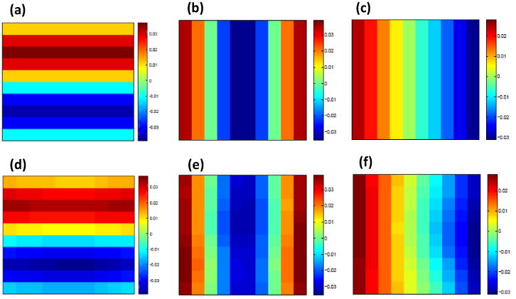
Simulation results from Study I: a selected slice of (a) true ψ₁(d, t); (b) true ψ₂(d, t); (c) true ψ₃(d, t); (d) ψ̂₁(d, t); (e) ψ̂₂(d, t); and (f) ψ̂₃(d, t).

We applied the three-stage estimation procedure described in Section 2.2 to the simulated data. First, we estimated the fixed main effect function μ(d, x_i(t)) using penalized smoothing spline implemented in the R package vows [Reiss et al., 2014]. Then we used a local linear regression to estimate η_i(d, t) based on the residuals y_i(d, t)−μ̂(d,x_i(t)). Following the method described in Section 2.2, we estimated the eigenvalues and eigenfunctions associated with the covariance function Σ_η((d, t), (d′, t′)). Figure 1 (a) shows the relative eigenvalues, where the relative eigenvalues are defined as the ratios of the eigenvalues over their sum. It is shown that the first three eigenvalues account for more than 90% of the total variation and the others quickly vanish to zero. We present some selected slices of the estimated eigenfunctions corresponding to the largest three eigenvalues along with the true eigenfunctions in Figure 2. It shows that the estimates are close to the true eigenfunctions, and η̂_i(d,t) can capture major variation in the true eigenfunctions. The parameters of the covariance model in Gneiting [2002] were estimated by following Stage (III) in Section 2.2.

Figure 1.

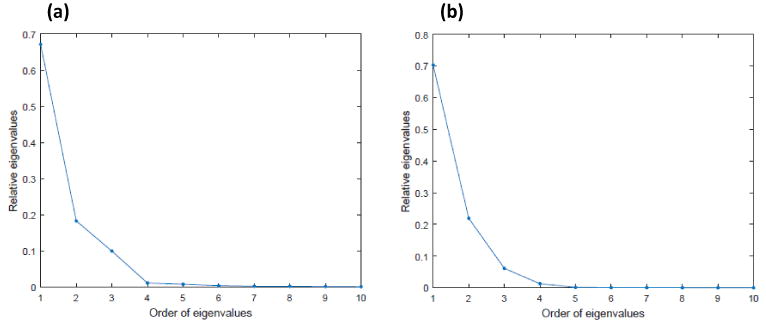
Simulation results: the first 10 relative eigenvalues of Σ̂_η((d, t), (d′, t′)) for (a) Study I and (b) Study II.

To evaluate the prediction accuracy of STGP, we split the simulated data set into a training set of 50 subjects and a test set of 30 subjects. Then we followed the prediction procedure in Section 2.3 to predict the image at the last time point for each of the 30 subjects in the test set, based on the first two images and the fitted model from the training set. We compared the predictive performance of STGP with those of the semiparametric model, which assumed the mean structure and uncorrelated errors, and the semiparametric model+FPCA. Table 1 shows the overall rtMSPE (14) for each model. As can be seen in Table 1, STGP outperforms the other two methods.

Table 1.

Simulation results. The overall rtMSPE was obtained for the simulated data in Study I.

Model	rtMSPE
Semiparametric model	0.0871
Semiparametric model+FPCA	0.0428
STGP	0.0395

3.2 Study II: random effects model approach

By mimicking the real imaging data in Section 4.2, we simulated data at all 900 pixels of a 30 × 30 phantom image for n = 24 subjects at different measurement times per subject. At a given pixel d = (d₁, d₂)^T, the data were generated from a spatio-temporal Gaussian process model according to

$$y_{i,k(d)}(d,t_{ij})=\mu (d,{\mathbf{x}}_i(t_{ij}))+{\eta }_i(d,t_{ij})+{\epsilon }_{i,k(d)}(d,t_{ij}),i=1,\dots ,24;j=1,\dots ,m_i.$$ (16)

We used the real data in Section 4.2 to specify x_i(t) = (x_i,1(t), x_i,2(t))^T and the fixed main effect function μ(d, x_i(t)), where the components of x_i(t) represent gender and age, respectively. We set ${\eta }_i(d,t)={\sum }_{l=1}^3{\xi }_{i,l}{\psi }_l(d,t)$, where ξ_i,l were independently generated according to ξ_i,1 ∼ N(0, 12²), ξ_i,2 ∼ N(0, 7²), and ξ_i,3 ∼ N(0, 4²). The eigenfunctions were chosen as follows:

$${\psi }_1(d,t)=\frac{\sqrt{2}}{45}sin(\pi (d_1+d_2)/15)cos(\pi t/18),{\psi }_2(d,t)=\frac{\sqrt{2}}{45}cos(\pi (d_1+d_2)/15)cos(\pi t/18),{\psi }_3(d,t)=\frac{1}{30\sqrt{3}}cos(\pi t/12).$$

Figure 3 (a)-(c) show the three eigenfunctions at baseline. We arbitrarily clustered all voxels into five mutually exclusive regions and simulated realizations of the zero-mean Gaussian process ε_i,k(d)(d,t) according to model (6). For the choice of the covariance function, we used a spatio-temporal autoregressive model [Derado et al., 2010], which extends the simultaneous autoregressive model in Hyun et al. [2014] to the spatio-temporal process context.

Figure 3.

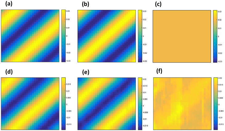
Simulation results from Study II: a selected slice of (a) true ψ₁(d, t); (b) true ψ₂(d, t); (c) true ψ₃(d, t); (d) ψ̂₁(d, t); (e) ψ̂₂(d, t); and (f) ψ̂₃(d, t).

Similarly to the simulation in Section 3.1, we applied almost the same estimation procedure in Section 2.2 to the simulated data except a minor difference. Specifically, since the simulated data are sparse with unequal number of repeated measurements and different measurement times per subject, we used the random effects model approach in Stage (II) of Section 2.2 to estimate η_i(d, t). Then, η̂_i(d, t) was used to obtain the estimates of eigenvalue-eigenfunction pairs associated with the covariance function Σ_η((d, t), (d′, t′)). The relative eigenvalues are shown in Figure 1 (b). Figure 3 shows the estimated eigenfunctions corresponding to the largest three eigenvalues along with the true eigenfunctions. Inspecting Figure 3 reveals that η̂_i(d, t) can faithfully recover the true eigenfunctions.

To examine the predictive performance of STGP, we randomly split the simulated data set into a training set of 16 subjects and a test set of 8 subjects. Then, we predicted the image at the last time point for each of the 8 subjects in the test set. The prediction results are summarized in Table 2, which shows that STGP performs well even when the longitudinal data are sparse with unequal number of repeated measurements and different measurement times per subject.

Table 2.

Simulation results. The overall rtMSPE was obtained for the simulated data in Study II.

Model	rtMSPE
Semiparametric model	0.4885
Semiparametric model+FPCA	0.4278
STGP	0.4256

4 Real data analysis

4.1 ADNI PET data

We applied our proposed method to PET scans obtained at baseline, 6 months, and 12 months obtained from 159 subjects in the Alzheimer's Disease Neuroimaging Initiative (ADNI) study. Among them, there are 50 Normal Controls (NC), 58 Mild Cognitive Impairments (MCI) and 51 Alzheimer's Disease (AD) subjects. There are 97 males, whose mean baseline age is 77 years with standard deviation 6 years, and 62 females, whose mean baseline age is 75.5 years with standard deviation 6.7 years. FDG-PET images acquired 30-60 minutes post-injection were processed by using a standard image processing pipeline. A detailed description of PET protocols and acquisition can be found at www.adni-info.org. Such pipeline consists of average, spatial alignment, interpolation to a standard voxel size, intensity normalization, and smoothing to a common resolution of 8-mm full width at half maximum. The dimension of the processed PET images is 79×95×69.

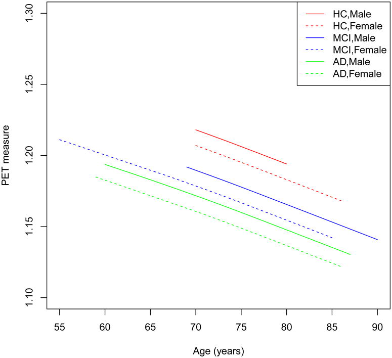
We applied the prediction procedure in Section 2.3 to the PET scans. We randomly selected 80 subjects for a training set and used their data to train the prediction model. We included gender, diagnostic status (HC, MCI, AD), and age as covariates of interest. We first fitted the spatio-temporal Gaussian process model to the training data to estimate the fixed main effect μ(d, x_i(t)), eigenvalue-eigenfunction pairs, and the model parameters in (6). Figure 4 presents the estimated μ̂(d, x_i(t)) as a function of age corresponding to six combinations of diagnostic status and gender in a randomly selected voxel. For subjects in each of the six combinations, PET measure linearly decreases as age increases. Moreover, we observe that PET measures have two interesting patterns with HC>MCI>AD and Male>Female.

Figure 4.

Results from the ADNI PET data in a randomly selected voxel: the fitted mean curves for (a) male NC subjects; (b) male MCI subjects; (c) male AD subjects; (d) female NC subjects; (e) female MCI subjects; and (f) female AD subjects.

The voxels were partitioned into 128 mutually exclusive brain regions by our clustering method. For smoothing of the mean function, we used penalized smoothing spline with smoothing parameters estimated by REML. In Figure 5 (a), we present the relative eigenvalues associated with the covariance function Σ_η((d, t), (d′, t′)), which decrease slowly to zero. We also show some selected slices of the estimated eigenfunctions corresponding to the largest four eigenvalues in Figure 6. We specified (6) using the nonseparable Gneiting's covariance model as in the simulated example and estimated the model parameters by optimizing (11).

Figure 5.

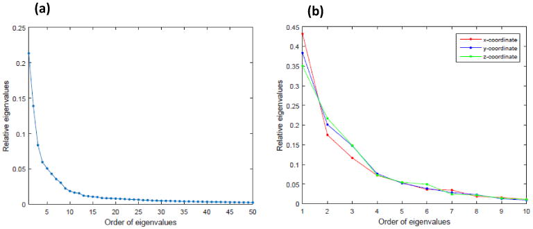
(a) The first 50 relative eigenvalues of Σ̂_η((d, t), (d′, t′)) for the ADNI data; and (b) The first 10 relative eigenvalues for the surface data.

Figure 6.

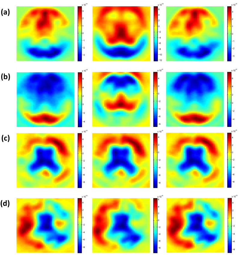
Results from the ADNI data: (a) ψ̂₁(d, t); (b) ψ̂₂(d, t); (c) ψ̂₃(d, t); and (d) ψ̂₄(d, t). Selected slices are shown.

The fitted model was then used to predict the PET scans at 12 months for each of the 79 subjects in the test set, based on the images at baseline and 6 months. Figure 7 shows the individual PET images predicted at 12 months (bottom panel) along with the corresponding observed images (upper panel) for three selected subjects consisting of an NC, an MCI, and an AD subject. We find that there is a strong agreement between the observed and predicted images.

Figure 7.

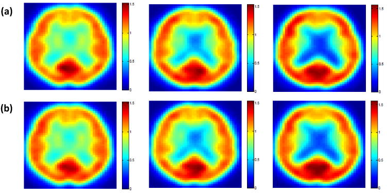
Results from the ADNI data: (a) observed and (b) predicted PET images at 12 months for an NC, an MCI, and an AD subject (from left to right). One selected slice is shown.

We evaluated the prediction accuracy of our proposed model by calculating the rtMSPE(d) (13) and compared the results for the proposed model with those for the semiparametric model and the semiparametric model+FPCA. Figure 8 shows the rtMSPE(d) maps for the three models. Inspecting Figure 8 reveals that STGP provided substantially better prediction performance than the other models. We also calculated the overall rtMSPE for each model and compared the results in Table 3. The overall rtMSPE was reduced by 49% using the proposed model compared with the semiparametric model, while it was reduced by 36% compared with the semiparametric model+FPCA. We find that STGP can substantially increase the prediction accuracy compared with the other two models.

Figure 8.

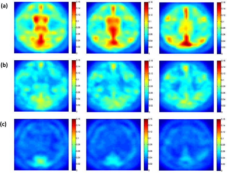
Results from the ADNI data: rtMSPE maps for predicting the PET scans at 12 months for 79 subjects in the test set. Selected slices are shown for (a) the semiparametric model; (b) the semiparametric model+FPCA; and (c) STGP.

Table 3.

Results from the ADNI data. The overall rtMSPE was obtained for predicting the PET scans at 12 months.

Model	rtMSPE
Semiparametric model	0.0692
Semiparametric model+FPCA	0.0550
STGP	0.0354

4.2 Lateral ventricle surface data

We considered a longitudinal lateral ventricle surface data set obtained from a study of early brain development [Bompard et al., 2014]. See Bompard et al. [2014] for detailed information on imaging acquisition and analysis. The surface data set includes measurements for 24 healthy full-term infants (12 males and 12 females) at months 0 (2 weeks), 3, 6, 9, 12 approximately, with different infants having different visiting times and some infants missing a visit. Informed consent was obtained from the parents of all participants, and the experimental protocols were approved by the Institutional Review Board, University of North Carolina at Chapel Hill.

All subjects were scanned on a 3T MR scanner (Siemens Medical System, Erlangen, Germany) housed in the Biomedical Research Imaging Center. The T2-weighted images used in this study were acquired using a turbo spin-echo (TSE) sequence: TR = 7380 ms, TE = 119 ms, Flip Angle = 150u, and resolution = 1.256 × 1.256 × 1.95mm³. A total of 70 slices were acquired to cover the entire brain. None of the subjects were sedated for MRI; all scans were performed with subjects during sleep. Subjects were fed before scanning, then swaddled, allowed to fall asleep, fitted with ear protection and their heads secured.

We applied a pre-processing pipeline to all T2-weighted images in order to segment lateral ventricles (LVs). Such pipeline includes removal of non-brain tissues such as the skull and dura using Brain Surface Extractor (BSE)[Shattuck and Leahy, 2001], bias correction using the non-parametric non-uniform intensity normalization (N3) method [Sled et al., 1998], and resampling to a resolution of 1 × 1 × 1mm³. Subsequently, we applied a longitudinal neonatal brain image segmentation algorithm [Shi et al., 2010] and then outlined the LV structures based on the segmented CSF maps. Finally, two observers performed manual correction of the lateral ventricle segmentation using the ITK-SNAP software [Yushkevich et al., 2006].

We applied the SPHARM-PDM [Styner et al., 2004] shape representation to establish surface correspondence and aligned the surface location vectors across all subjects. The sampled SPHARM-PDM is a smooth, accurate, fine-scale shape representation. The left lateral ventricle surface of each infant is represented by 1002 location vectors with each location vector consisting of the spatial x, y, and z coordinates of the corresponding vertex on the SPHARM-PDM surface.

We applied the prediction procedure in Section 2.3 to the spatial x, y, and z coordinates on the SPHARM-PDMs of the left lateral ventricle. Our analysis included the SPHARM-PDM representation of left lateral ventricle surfaces as responses and gender and age (in months) as covariates. We randomly selected 16 infants for a training set and fitted STGP to the training set. We estimated μ(d, x_i(t)) by using penalized smoothing spline. Figure 9 presents observed individual trajectories of the surface location vectors and their corresponding estimated curves μ̂(d, x_i(t)) as functions of age across gender on a randomly selected vertex. Overall, most of these estimated curves μ̂(d, x_i(t)) increase initially and slow down around 10 months.

Figure 9.

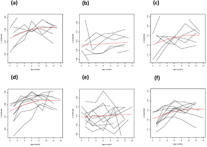
Results from the surface data on a randomly selected vertex: Observed individual trajectories of the surface location vectors and the smooth estimates of the mean function for (a) x-coordinate for male infants; (b) y-coordinate for male infants; (c) z-coordinate for male infants; (d) x-coordinate for female infants; (e) y-coordinate for female infants; and (f) z-coordinate for female infants.

Since different subjects have different measurement times and unequal number of repeated measurements, we estimated eigenvalue-eigenfunction pairs by using the random effects model approach described in Section 2.2. The relative eigenvalues are shown in Figure 5 (b). To characterize the local correlation, we partitioned the voxels on the SPHARM-PDM surface into 5 mutually exclusive regions by using our clustering method based on a Gaussian mixture model and specified the covariance function (6) using a spatio-temporal autoregressive model as illustrated in Section 3.2. The unknown parameters in (6) were estimated by REML.

We used the fitted model to predict the x, y, and z coordinates at the last time point for each of the 8 infants in the test set, based on their spatial coordinates at earlier time points. We compare the individual predicted spatial coordinates with the observed coordinates for three randomly selected subjects in Figure 10. To evaluate the predictive performance, we calculated the rtMSPE(d) for the x, y, and z coordinates, respectively. The results are shown in Figure 11 for the proposed model along with those for the semiparametric model and the semiparametric model+FPCA. Figure 11 shows that STGP improves upon the other two models. We also calculated the overall rtMSPE for each model and present the results in Table 4. The overall rtMSPE was reduced by 19 to 32% using STGP compared with the semiparametric model, while it was also reduced by 9 to 11% compared with the semiparametric model+FPCA. With the limited number of subjects, the improvements decrease compared with the results in Section 4.1, but nevertheless STGP outperformed the other two models.

Figure 10.

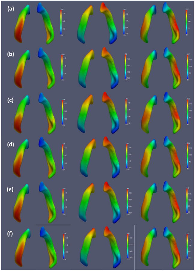
Results from the surface data: (a) observed and (b) predicted coordinates for Subject 4; (c) observed and (d) predicted coordinates for Subject 5; (e) observed and (f) predicted coordinates for Subject 6. The x, y, and z coordinates are shown from left to right.

Figure 11.

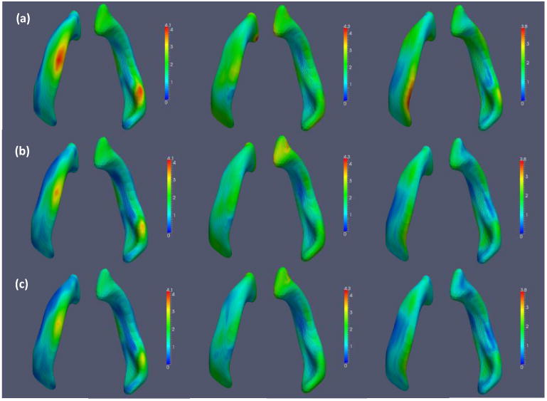
Results from the surface data: rtMSPE maps for predicting the spatial coordinates at the last time points for 8 subjects in the test set. The x, y, and z coordinates are shown from left to right for (a) semiparametric model; (b) semiparametric model+FPCA; and (c) STGP.

Table 4.

Results from the surface data. The overall rtMSPE was obtained for predicting the spatial coordinates at the last time points.

Model	rtMSPE
	x-coordinate	y-coordinate	z-coordinate
Semiparametric model	1.6111	1.8847	1.5674
Semiparametric model+FPCA	1.3175	1.6999	1.1959
STGP	1.2022	1.5199	1.0730

5 Discussion

We have proposed a spatio-temporal Gaussian process framework for modeling neuroimaging data from longitudinal studies. We have developed a three-stage estimation procedure and a predictive method based on STGP. We have applied the proposed model to two real data analyses including longitudinal positron emission tomography data and longitudinal lateral ventricle surface data to show that our approach can substantially improve predictive performance compared with some existing methods.

Our approach provides a computationally efficient framework for approximating the unstructured variance-covariance matrix of ultra-high dimensional data by explicitly modeling the long-to-medium-to-short-range spatio-temporal dependence. The computational cost for the estimation of the mean function and the FPCA model is relatively low while the optimization of the REML function takes most of the computing time. For the ADNI PET data in Section 4.1, it took about 4 hours to optimize the REML function for the largest brain region. The computing time for the optimization over the entire domain is significantly reduced when it is implemented in a parallel manner.

An important issue with our partition covariance model is that one needs to choose the number of partitioned brain regions. In our examples, the partition was created in a way that the number of voxels in each subregion is not too large in order to reduce the computational cost. More research on the selection of this tuning parameter is needed. It is also interesting to extend our FPCA model to incorporate covariates. Our proposed model incorporates the effect of the covariates through the mean function, but the influence of the predictor can also be incorporated through the random components of a functional principal components expansion [Chiou et al., 2004]. It would be interesting to investigate the predictive abilities of various models with a covariate effect either on the mean function or on the residual process.

Another important issue is to check the key assumptions of the proposed spatio-temporal Gaussian process. Specifically, we may develop various diagnostic measures (e.g., residuals, local influence measure, residual process and test statistics) to systematically test the mean structure in (1) and examine potential outliers and influential points. Subsequently, we will examine the assumption of FPCA by examining whether FPCA is an efficient method for capturing major variation in longitudinal functional data. Finally, we can use local spectral frequency plots to investigate the short-range correlation structure of neuroimaging data.

References

- Almli CR, Rivkin MJ, McKinstry RC Group., B. D. C. The nih mri study of normal brain development (objective-2): newborns, infants, toddlers, and preschoolers. IEEE Transactions on Medical Imaging. 2007;35:308–325. doi: 10.1016/j.neuroimage.2006.08.058. [DOI] [PubMed] [Google Scholar]
- Ashburner J, Ridgway GR. Symmetric diffeomorphic modeling of longitudinal structural mri. Frontiers in neuroscience. 2012;6 doi: 10.3389/fnins.2012.00197. [DOI] [PMC free article] [PubMed] [Google Scholar]
- Bernal-Rusiel J, Greve D, Reuter M, Fischl B, Sabuncu MR. Statistical analysis of longitudinal neuroimage data with linear mixed effects models. NeuroImage. 2013;66:249–260. doi: 10.1016/j.neuroimage.2012.10.065. [DOI] [PMC free article] [PubMed] [Google Scholar]
- Bompard L, Xu S, Styner M, Paniagua B, Ahn M, Yuan Y, Jewells V, Gao W, Shen D, Zhu H, et al. Multivariate longitudinal shape analysis of human lateral ventricles during the first twenty-four months of life. 2014 doi: 10.1371/journal.pone.0108306. [DOI] [PMC free article] [PubMed] [Google Scholar]
- Brezger A, Fahrmeir L, Hennerfeind A. Adaptive gaussian markov random fields with applications in human brain mapping. Journal of the Royal Statistical Society: Series C (Applied Statistics) 2007;56(3):327–345. [Google Scholar]
- Chiou JM, Müller HG, Wang JL, et al. Functional response models. Statistica Sinica. 2004;14:675–694. [Google Scholar]
- Cressie N, Wikle CK. Statistics for Spatio-temporal Data. John Wiley & Sons; 2011. [Google Scholar]
- Demel SS, Du J. Spatio-temporal models for some data sets in continuous space and discrete time. Statistica Sinica. 2015;25:81–98. [Google Scholar]
- Derado G, Bowman FD, Kilts CD. Modeling the spatial and temporal dependence in fmri data. Biometrics. 2010;66(3):949–957. doi: 10.1111/j.1541-0420.2009.01355.x. [DOI] [PMC free article] [PubMed] [Google Scholar]
- Derado G, Bowman FD, Zhang L. Predicting brain activity using a bayesian spatial model. Statistical methods in medical research. 2013;22(4):382–397. doi: 10.1177/0962280212448972. [DOI] [PMC free article] [PubMed] [Google Scholar]
- Evans AC Group., B. D. C. The nih mri study of normal brain development. NeuroImage. 2006;30:184–202. doi: 10.1016/j.neuroimage.2005.09.068. [DOI] [PubMed] [Google Scholar]
- Fan J, Gijbels I. Local Polynomial Modelling and Its Applications. Chapman and Hall; London: 1996. [Google Scholar]
- Gneiting T. Nonseparable, stationary covariance functions for space–time data. Journal of the American Statistical Association. 2002;97(458):590–600. [Google Scholar]
- Gössl C, Auer DP, Fahrmeir L. Bayesian spatiotemporal inference in functional magnetic resonance imaging. Biometrics. 2001;57(2):554–562. doi: 10.1111/j.0006-341x.2001.00554.x. [DOI] [PubMed] [Google Scholar]
- Greven S, Crainiceanu C, Caffo B, Reich B. Longitudinal functional principal components analysis. Electronic Journal of Statistics. 2010;4:1022–1054. doi: 10.1214/10-EJS575. [DOI] [PMC free article] [PubMed] [Google Scholar]
- Guillaume B, Hua X, Thompson PM, Waldorp L, Nichols TE. Fast and accurate modelling of longitudinal and repeated measures neuroimaging data. NeuroImage. 2014;94:287–302. doi: 10.1016/j.neuroimage.2014.03.029. [DOI] [PMC free article] [PubMed] [Google Scholar]
- Guo Y, DuBois Bowman F, Kilts C. Predicting the brain response to treatment using a bayesian hierarchical model with application to a study of schizophrenia. Human brain mapping. 2008;29(9):1092–1109. doi: 10.1002/hbm.20450. [DOI] [PMC free article] [PubMed] [Google Scholar]
- Hall P, Müller HG, Wang JL. Properties of principal component methods for functional and longitudinal data analysis. The Annals of Statistics. 2006;34:1493–1517. [Google Scholar]
- Hong Y, Joshi S, Sanchez M, Styner M, Niethammer M. Medical Image Computing and Computer-Assisted Intervention–MICCAI 2012. Springer; 2012. Metamorphic geodesic regression; pp. 197–205. [DOI] [PMC free article] [PubMed] [Google Scholar]
- Huang C, Styner M, Zhu H. Clustering high-dimensional landmark-based two-dimensional shape data. Journal of the American Statistical Association. 2015;110(511):946–961. doi: 10.1080/01621459.2015.1034802. [DOI] [PMC free article] [PubMed] [Google Scholar]
- Hyun JW, Li Y, Gilmore JH, Lu Z, Styner M, Zhu H. Sgpp: spatial gaussian predictive process models for neuroimaging data. NeuroImage. 2014;89:70–80. doi: 10.1016/j.neuroimage.2013.11.018. [DOI] [PMC free article] [PubMed] [Google Scholar]
- Kim P, Leckman JF, Mayes L, Feldman R, Wang X, Swain JE. The plasticity of human maternal brain: longitudinal changes in brain anatomy during the early postpartum period. Behavioral Neuroscience. 2010;124:695–700. doi: 10.1037/a0020884. [DOI] [PMC free article] [PubMed] [Google Scholar]
- Li Y, Gilmore JH, Shen D, Styner M, Lin W, Zhu HT. Multiscale adaptive generalized estimating equations for longitudinal neuroimaging data. NeuroImage. 2013;72:91–105. doi: 10.1016/j.neuroimage.2013.01.034. [DOI] [PMC free article] [PubMed] [Google Scholar]
- Lorenzi M, Ziegler G, Alexander DC, Ourselin S. Efficient gaussian process-based modelling and prediction of image time series. IPMI 2015. 2015 doi: 10.1007/978-3-319-19992-4_49. [DOI] [PMC free article] [PubMed] [Google Scholar]
- Marco L, Gabriel Ziegler G, Alexander DC, Ourselin S. Modelling non-stationary and non-separable spatio-temporal changes in neurodegeneration via gaussian process convolution. 1st ICML Workshop on Machine Learning Meets Medical Imaging 2015 [Google Scholar]
- Meltzer JA, Postman-Caucheteux W, McArdle JJ, Braun A. Strategies for longitudinal neuroimaging studies of overt language production. Neuroimage. 2009;47:745–755. doi: 10.1016/j.neuroimage.2009.04.089. [DOI] [PMC free article] [PubMed] [Google Scholar]
- Pan W, Shen X. Penalized model-based clustering with application to variable selection. J Mach Learn Res. 2007;8:1145–1164. [Google Scholar]
- Penny WD, Trujillo-Barreto NJ, Friston KJ. Bayesian fmri time series analysis with spatial priors. NeuroImage. 2005;24(2):350–362. doi: 10.1016/j.neuroimage.2004.08.034. [DOI] [PubMed] [Google Scholar]
- Reiss PT, Huang L, Chen YH, Huo L, Tarpey T, Mennes M. Massively parallel nonparametric regression, with an application to developmental brain mapping. Journal of Computational and Graphical Statistics. 2014;23(1):232–248. doi: 10.1080/10618600.2012.733549. [DOI] [PMC free article] [PubMed] [Google Scholar]
- Ruppert D, Wand MP, Carroll RJ. Semiparametric regression. Number 12. Cambridge university press; 2003. [Google Scholar]
- Shattuck DW, Leahy RM. Automated graph-based analysis and correction of cortical volume topology. Medical Imaging, IEEE Transactions on. 2001;20(11):1167–1177. doi: 10.1109/42.963819. [DOI] [PubMed] [Google Scholar]
- Shi F, Fan Y, Tang S, Gilmore JH, Lin W, Shen D. Neonatal brain image segmentation in longitudinal mri studies. Neuroimage. 2010;49(1):391–400. doi: 10.1016/j.neuroimage.2009.07.066. [DOI] [PMC free article] [PubMed] [Google Scholar]
- Singh N, Hinkle J, Joshi S, Fletcher PT. Hierarchical geodesic models in diffeomorphisms. International Journal of Computer Vision. 2015:1–23. [Google Scholar]
- Skup M, Zhu H, Zhang H. Multiscale adaptive marginal analysis of longitudinal neuroimaging data with time-varying covariates. Biometrics. 2012;68:1083–1092. doi: 10.1111/j.1541-0420.2012.01767.x. [DOI] [PMC free article] [PubMed] [Google Scholar]
- Skup M, Zhu HT, Wang Y, Giovanello KS, Lin JA, Shen DG, Shi F, Gao W, Lin W, Fan Y, Zhang HP ADNI. Sex differences in grey matter atrophy patterns among ad and amci patients: Results from adni. NeuroImage. 2011;56:890–906. doi: 10.1016/j.neuroimage.2011.02.060. [DOI] [PMC free article] [PubMed] [Google Scholar]
- Sled JG, Zijdenbos AP, Evans AC. A nonparametric method for automatic correction of intensity nonuniformity in mri data. Medical Imaging, IEEE Transactions on. 1998;17(1):87–97. doi: 10.1109/42.668698. [DOI] [PubMed] [Google Scholar]
- Styner M, Lieberman JA, Pantazis D, Gerig G. Boundary and medial shape analysis of the hippocampus in schizophrenia. Medical Image Analysis. 2004;8:197–203. doi: 10.1016/j.media.2004.06.004. [DOI] [PubMed] [Google Scholar]
- Weiner MW, Veitch DP, Aisen PS, Beckett LA, Cairns NJ, Green RC, Harvey D, Jack CR, Jagust W, Liu E, et al. The alzheimer's disease neuroimaging initiative: a review of papers published since its inception. Alzheimer's & Dementia. 2013;9(5):e111–e194. doi: 10.1016/j.jalz.2013.05.1769. [DOI] [PMC free article] [PubMed] [Google Scholar]
- Woolrich MW, Jenkinson M, Brady JM, Smith SM. Fully bayesian spatio-temporal modeling of fmri data. Medical Imaging, IEEE Transactions on. 2004;23(2):213–231. doi: 10.1109/TMI.2003.823065. [DOI] [PubMed] [Google Scholar]
- Yao F, Lee T. Penalized spline models for functional principal component analysis. Journal of the Royal Statistical Society: Series B (Statistical Methodology) 2006;68:3–25. [Google Scholar]
- Yuan Y, Gilmore JH, Geng X, Styner M, Chen K, Wang JL, Zhu H. A longitudinal functional analysis framework for analysis of white matter tract statistics. In: Wells WM, Joshi SS, Pohl KM, editors. LNCS7917. Springer; Berlin/Heidelberg: 2013. pp. 220–231. Information Processing in Medical Imaging. [DOI] [PMC free article] [PubMed] [Google Scholar]
- Yushkevich PA, Piven J, Hazlett HC, Smith RG, Ho S, Gee JC, Gerig G. User-guided 3d active contour segmentation of anatomical structures: significantly improved efficiency and reliability. Neuroimage. 2006;31(3):1116–1128. doi: 10.1016/j.neuroimage.2006.01.015. [DOI] [PubMed] [Google Scholar]