De novo deciphering three-dimensional chromatin interaction and topological domains by wavelet transformation of epigenetic profiles

Abstract

Defining chromatin interaction frequencies and topological domains is a great challenge for the annotations of genome structures. Although the chromosome conformation capture (3C) and its derivative methods have been developed for exploring the global interactome, they are limited by high experimental complexity and costs. Here we describe a novel computational method, called CITD, for de novo prediction of the chromatin interaction map by integrating histone modification data. We used the public epigenomic data from human fibroblast IMR90 cell and embryonic stem cell (H1) to develop and test CITD, which can not only successfully reconstruct the chromatin interaction frequencies discovered by the Hi-C technology, but also provide additional novel details of chromosomal organizations. We predicted the chromatin interaction frequencies, topological domains and their states (e.g. active or repressive) for 98 additional cell types from Roadmap Epigenomics and ENCODE projects. A total of 131 protein-coding genes located near 78 preserved boundaries among 100 cell types are found to be significantly enriched in functional categories of the nucleosome organization and chromatin assembly. CITD and its predicted results can be used for complementing the topological domains derived from limited Hi-C data and facilitating the understanding of spatial principles underlying the chromosomal organization.

INTRODUCTION

The genome is hierarchically organized in three-dimensional (3D) space inside the cell nucleus and exhibits multiple layers of functional complexity, including chromosomal territories, megabase-long topological domains and DNA loops among cis-regulatory elements (e.g. enhancers and promoters). To comprehensively understand the relationship of genome structures and functions is an important but extremely difficult technical challenge (1–3). Newly developed biochemical approaches (such as 3C, 4C, 5C, Hi-C and ChIA-PET) have been applied to explore physical interaction frequency that was defined as the probability of a pair of chromosomal loci interacting with each other among a large cell population (4–7). However, these methods largely rely on chemical cross-linking, DNA–DNA proximity ligation and enzyme digestion (or sonication), which lead to link uncertainty (noise), less of quantitative control and high experimental complexity (4,7–9). Additionally, current technologies are limited to measure high-order chromosome organizations while simultaneously achieving higher resolutions. A detailed and comprehensible description of the 3D genome organization and function will require the development of computational technologies that can reveal such complex hierarchical organization at different physical scales.

Epigenetic modifications, such as DNA methylation and the chemical modifications on nucleosomal histones H2A, H2B, H3 and H4, play key roles in epigenetic regulation of chromatin structure and gene expression (5,10). Histone modifications (e.g. acetylation, methylation, phosphorylation and ubiquitylation) can result in different functional outcomes depending on the different modified sites, the modification degrees and in what combinations (11–14). Large-scale mapping of histone modifications has emerged as a powerful means for characterizing the chromatin structures/states, since chromatin regulators and histone modifications work in conjunction with other co-factors to silence or to activate broad genomic regions (15,16). For example, large-scale repressions of megabase domains are correlated with H3K9me2 and H3K9me3 (17–19). Different combinations and patterns of various histone modifications have been widely observed to be associated with specific genomic regions (13,20). Integrative analysis of these epigenetic modifications had been successfully used to annotate chromatin states (21–23), genomic A/B compartments (24) and topological domain boundaries (25). Recent research of Hi-C experiments from multi species reported that two neighboring loci within a topologically associating domain (TAD), as opposed to a pair of arbitrary loci, usually have similar chromatin modifications patterns and strong interaction frequencies (26), indicating potential relationship between chromatin interaction and epigenetic modifications. Computationally, for each chromosomal locus, we can calculate an average enrichment for each of the modifications and create a vector representing the enrichment of all modifications. High similarity of epigenetic modification patterns at two loci can be quantitatively translated to a high correlation value between their vectors. However, the correlation of chromatin modification patterns does not always imply interaction frequency. Two distant chromosomal loci (e.g. two promoter regions) may display similar epigenetic modifications and hence a high correlation, but may not necessarily imply the presence of their interaction. Considering that chromatin interaction frequencies decline as the distance increases (following a power law) (7), we can accordingly transform the correlations of histone modifications among chromosomal loci so that they will closely follow the same power law. Thus the transformed correlation of histone modifications can be considered as surrogates for chromatin interaction frequencies, and consequently can be used for segmenting topological domains.

Motivated by the aforementioned observations, we developed a computational method to estimate chromatin interaction frequency from one-dimensional (1D) histone modifications. For the purposes of benchmarking, we compared our predictions with interactions and TADs obtained from Hi-C experiments of IMR90 and H1 cell lines. The cross-chromosome and cross-cell-type testing as well as case studies show that CITD can be used to estimate the landscape of interactions as Hi-C data. We further applied CITD to 98 additional cell types of Roadmap Epigenomics (27) and ENCODE project (28) to generate systematic predictions of chromatin interaction frequencies, topological domains and their states (active or repressive). These comprehensive results may enable us to uncover preserved domain boundaries and to delineate underlying mechanisms of chromosomal reorganization during human embryonic stem cell differentiation.

MATERIALS AND METHODS

Datasets

Hi-C dataset

The Hi-C interaction matrices of IMR90 and H1 cell lines were downloaded from GEO under accession number GSE35156. The TAD were downloaded from Hi-C project database (http://yuelab.org/hi-c/). For both cells, the chromosomal positions of Hi-C results were based on reference human version of GRCh36/hg18.

Histone modifications

The dataset of histone modifications were downloaded from Roadmap Epigenomics project (27) and ENCODE project (28). A total of 84 cell types were downloaded from Roadmap Epigenomics project at NCBI database (www.ncbi.nlm.nih.gov/geo.roadmap/epigenomics) and 16 cell types were downloaded from ENCODE project under accession number GSE29611 (see Supplementary Table S1 in Supplementary Data File 1 for a complete list of cell types). For each cell type, the wig files of histone modifications were used to calculate the signal depth of modifications. The IMR90 cell has the most abundant modification set of 28 markers. The H1 cell has 27 different modifications and other cells have at least 10 histone modifications. All the modifications of IMR90 and H1 were mapped to reference human genome version GRCh36/hg18 and GRCh37/hg19. The other cell types were only mapped to reference human genome GRCh37/hg19. The results based on GRCh36/hg18 are only used for training and comparison with previous Hi-C data since they were only available for this version.

Transcriptional factors binding signals

The binding signals (wig format) of 10 transcriptional factors (IMR90) were downloaded from ENCODE project under accession numbers GSE31477 and GSE32465, including CTCF (GSM935404), POL2 (GSM935513), CHD1 (GSM1003623), MAFK (GSM935403), MXI1 (GSM1003614), RFX5 (GSM1003615), CEDPB (GSM935519), RAD21 (GSM935624), COREST (GSM1003612) and MAZ (GSM1003613). The signals of chromatin accessibility were downloaded from GEO with accession numbers GSM530665 and GSM530666. The signals of DNA methylation were downloaded from GEO with accession numbers GSM432687-432692. All histone modifications and binding signals were processed by subtracting the corresponding input control.

Transcriptome data

The transcriptome of IMR90 was downloaded from GEO database under accession number GSM438363. Reads were mapped to GRCh36/hg18 (NCBI GTF annotation) by using Bowtie software 1.0.1 release (29) and the gene FPKMs were called by using Cufflinks software 2.2.1 release (30) with default parameters.

CITD method

To provide scalable and effective predictions of chromatin interaction frequencies, CITD employed the following five steps to transform the multiple histone modifications into chromosome-based interaction matrices (Figure 1A).

Figure 1.

The CITD overview. (A) Constructing chromatin interaction frequency by wavelet transformation of histone modifications. ‘A’ means the approximation coefficients matrix. ‘H’, ‘V’ and ‘D’ mean horizontal, vertical and diagonal details coefficients matrices, respectively. First, the training data (Hi-C interaction matrices) and correlation matrix were decomposed by level one wavelet decomposition. The four coefficient matrices obtained from correlation matrix were optimized to be as similar as those from Hi-C matrix by following non-linear transformation (power law). The optimized coefficient matrices were then used to construct the interaction matrix by wavelet reconstruction. A hidden Markov model (HMM) method was followed to predict the topological domains. A classification method was used to predict the state of domain as active or repressive. (B) CITD was applied on total 100 cell types with scalable resolutions. The vertical and horizontal comparisons were performed among these cell types at different resolutions.

1. Data processing: for a given bin size, chromosomes are divided into bins. For each bin, the average ChIP-seq intensity value of all histone modifications are calculated and ordered as a numerical vector.

2. Calculation of Pearson correlation: for two vectors corresponding to any bin pair i and j, calculate the absolute value of the Pearson correlation. All pairs resulted in a correlation matrix.

3. Wavelet decomposition: for a chromosome region, the Hi-C matrix and correlation matrix are both decomposed into coefficient matrices that are corresponding to different frequency bands (31). The symmetric and biorthogonal wavelet filters (bio3.7) was used in the decomposition as it is widely used for 2D signal processing (32). The decompositions were performed on different levels from 1 to log₂L, which is the theoretical upper bound of wavelet decomposition for a matrix of size L. At each decomposition level n (n is an integer and ), there will be 3n + 1 coefficient matrices (31).

4. Non-linear transformation: for each coefficient matrix pair, namely Hi-C matrix and correlation matrix at level n and , non-linear transformation was used to transform into 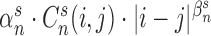. Here the scale parameter and the power parameter are optimized by minimizing the difference (least-square fit) as .

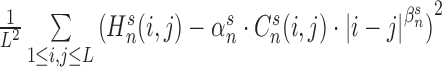5. Wavelet reconstruction: at each level n, the predicted matrix of chromatin interaction matrix was obtained by using wavelet reconstruction based on optimized coefficient matrix .

Training and optimizing parameters

To optimize the parameters, we used Hi-C matrices of IMR90 and H1 for training and testing by using a repeated random subsampling approach (Monte Carlo Cross-testing) (33). This approach randomly and equally split the 22 chromosomes into training and testing chromosomes. For each split, a chromosomal region with the size of 20 Mb was randomly selected from training chromosomes to optimize parameters, and a chromosomal region with the same size was randomly selected from the testing chromosomes for testing the performance. To minimize biases and over-fitting, the random splits were repeated 1000 times. We first applied this training-testing approach, referred as cross-chromosome testing, to both IMR90 and H1 cell types individually. We then trained parameters from IMR90 cell and tested them on seven cell types, and call this cross-cell-type testing.

Cross-chromosome testing

First, a chromosomal region of 20 Mb was randomly selected and 20 Mb is almost equal to the size of the smallest human chromosome. The Hi-C matrix and a correlation matrix of this region were used to optimize the best decomposition level and parameters for non-linear transformation.

1. Determining the best decomposition level. For a selected region of training chromosomes (IMR90 or H1), the difference between transformed matrix and Hi-C matrix H was calculated as for all possible decomposition levels . The standardized difference was then calculated as 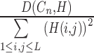, which is used to measure the relative difference of and H. We calculated the standardized differences at each decomposition level n. We repeated this process for 1000 times on both IMR90 and H1 individually. The optimized decomposition level was selected as the level n that obtains the minimal . Results show, for both IMR90 and H1 cells, level one decomposition (n = 1) obtained the smallest standardized differences (Supplementary Figure S1A in Supplementary Data File 2).

2. Parameter training for non-linear transformation. With the level one decomposition being the best, we then optimize the parameters for non-linear transformation. For a selected chromosome region of IMR90 or H1, its Hi-C matrix and correlation matrix were processed with wavelet decomposition of level one and each matrix resulted into four coefficient matrices that are corresponding to different signal frequencies. For each coefficient matrix pair of and , parameters and are optimized by minimizing the difference . The final eight parameters were calculated as the average of the parameters of total 1000 training processes.

3. Testing. These eight parameters were then tested on a randomly selected region of 20 Mb from testing chromosomes. For the selected testing region, the interaction matrix was calculated with trained eight parameters and the standardized difference was calculated by comparing it with the Hi-C matrix of this chromosomal region.

Cross-cell-type testing

To test if the trained parameters from one cell type can be applied to different cells, we did the cross-cell-type testing on seven cell types (H1, GM12878, NHEK, K562, HUVEC, HeLa and KBM7). For one of the seven cell types, we randomly selected 1000 regions from 22 chromosomes. For a selected region, the interaction matrix was calculated using these trained 8 parameters from IMR90. The standardized difference was calculated by comparing it with the Hi-C matrix of this region.

Testing different modification combinations

Currently, different cells had different number of histone modification types available. To test if our method can be used on different number of histone modification types, we randomly selected subsets from 28 modification types of IMR90 and repeated our predictions. For each random subset, the standardized difference was calculated and compared with the standardized difference obtained by using all 28 modifications. Since it is impossible to calculate all combinations, we sampled and calculated the combinations for . For each combination of n histone modifications we randomly repeated 1000 times with randomly selected regions of size 20 Mb. In real applications, we performed CITD on 100 cell types that have at least 10 modification types using the optimized parameter from IMR90 cell.

Predicting topological domains

Based on the predicted chromatin interaction matrix, we calculated the topological domains using Dixon's Method (based on HMM model) with the same parameters used for the Hi-C data of IMR90 and H1 (4). The topological domains with different resolutions of 40, 30, 20 and 10 kb are performed on each of the 100 cell types. For IMR90 and H1 cells, the predictions were calculated by using both reference human genome version GRCh36/hg18 and GRCh37/hg19. The predicted results based on GRCh37/hg18 were only used for comparison with previous results that were directly calculated from Hi-C data. All other cells were predicted by using the GRCh37/hg19 version. To compare the interaction strengths of domains, we calculated the average interaction of a domain as the average interaction frequency of its corresponding interaction matrix M (Hi-C interaction matrix or CITD predicted interaction matrix) that was defined as , where is the matrix size.

Predicting domain states

We built a classification-based method to better understand the active or repressive states of topological domains by analyzing the histone modifications. The utility of this step is 2-fold: first, by investigating the state of domains using histone modifications, we can provide additional benefits of our CITD method that started from same histone modification datasets. The second powerful aspect of the classification step is that it allows us to assess the state switches at TAD domain-level. The method was built as follows. (1) For a given domain, a score of each modification was constructed by averaging the raw values of the 40 kb bins included within this domain. For multiple modifications, a score vector then can be constructed. (2) Using those domain score vectors, K-means clustering algorithm implemented in Matlab was used to classify all domains into two classes. (3) The active and repressive states were indicated by the values of active modifications (H3K4me3, H3K36me3, H3K27ac, H3K79me1) and repressive modifications (H3K27me3, H3K9me3), respectively. For a domain, if the averaged value of active modifications is bigger than averaged value of repressive modifications, it is identified as an active domain. Otherwise, it is identified as a repressive domain. The active or repressive states were predicted for all the CITD predicted TAD domains of 100 cell types. We then defined two criteria as repressive ratio and alternating ratio to characterize the spatial distribution of domain states along chromosomes. The repressive ratio is defined as the fraction of repressed domains among total domains. The alternating ratio is defined as the fraction of neighboring domain pair with different domain state among total neighboring domain pairs. Using these two criteria, we can not only qualitatively measure the switches of domain states, but also quantitatively analyze their alternation patterns along spatial locations, and then facilitate the comparative analysis among cell types.

Comparative, statistical and functional analysis

Statistical analysis

The predicted topological domains of IMR90 and H1 were compared with the results obtained from their respective Hi-C data. K-S test was used to test the similarity of the number and length distributions between our predicted domains and Hi-C predicted ones on 22 chromosomes. CITD predictions were compared to the TAD domains for further performance analysis. In detail, we aligned CITD predicted domains to the TADs to identify the best match and calculated the overlap ratio, which is defined as the proportion of overlapped region over the TAD domain size. If one CITD prediction covers several TAD domains, only the longest TAD was kept and the overlap ratios of others were discarded. A TAD boundary is considered a match if a predicted boundary is located within 20% of the domain size. For each bin, we counted the frequency that this bin was predicted as a boundary among 100 cells, and achieved the boundary distribution of all bins along 22 chromosomes. The super preserved boundaries were defined as those that were predicted as boundaries in more than 90 cell types (as critical as 1% percentile of the boundary distribution). For a domain, the values of all its bins were calculated for each of 28 modifications to obtain the modification distributions of this domain. The K-S test was then used to test how similar are the distributions of each 28 modifications on neighboring domains.

Comparing with the results of PreSTIGE (34)

We downloaded 20190 enhancer–promoter interactions of H1 cell type predicted by PreSTIGE (version 1.0.0; http://mendel.gene.cwru.edu:8080). We analyzed the interaction scores of these enhancer–promoter interactions in our predictions. For a pair of enhancer and promoter, we first extracted a CITD predicted interaction score by using the two bins where they are located. For these 20190 enhancer–promoter interactions, we consider if they are enriched in top-ranked proportion of all CITD prediction scores. For a threshold of proportion θ (ranged from 1 to 100), we define recall as the fraction of the enhancer–promoter interactions with higher scores (ranked in θ% of CITD prediction scores) among all 20190 interactions.

Cell interaction entropy analysis

For an interaction matrix M of a chromosome, the values of its elements were discrete into 256 score levels from 0 to 255. Its entropy is defined as , where and x_i is the number of matrix elements with values falling in between i-1 to i score levels. Here the higher means lower consistence. The interaction entropy of a cell type is defined as the sum of the matrix entropy of all 22 chromosomes.

Functional analysis

The functional enrichment analysis and annotation of gene set were performed by DAVID database (35) and BINGO with release version 2.44 (36). The information were then manually verified and modified by using GeneCards database (37). For the 78 super boundaries, the protein–coding genes that located in ±40 kb regions were extracted by using the position file Refseq GTF (NCBI database, May 2014). The long non-coding RNA (lncRNA) were downloaded from LNCipedia database (version LNCipedia_3.0, released 28 August 2014), including 80216 high confident records (38). The non-coding RNA genes were downloaded from NONCODEv4 database (version 4.0, released 18 August 2014), including 145331 records (39). Non-coding genes (lncRNA, miRNA and others) that located in ±40 kb regions of 78 super boundaries were then extracted.

Delineating housekeeping gene

Housekeeping genes were identified by using the expression data of 84 tissues (or cells) from database BioGPS (September 2014) (40). The definition and calculation were the same as early studies (4). Given a gene x with expression in a given tissue i, the entropy gene expression is calculated as , where is the probability of in tissue i and N is the total number of tissues. High entropy scores have relatively uniform expression patterns and considered to be housekeeping genes. Here a threshold was taken as 6.5 that indicates the gene x has uniform expressions in at least 70 tissues as used in early study (4).

RESULTS

The CITD method

To predict chromatin interaction frequencies and topological domains, we explored two biological observations. (i) The histone modifications at a pair of interacting loci are correlated; (ii) the chromatin interaction frequencies decline with chromosomal distance following a power law. We implemented the observations to develop a computational method, CITD, to infer cell-type specific chromatin interaction matrices (Figure 1A). CITD first divided the chromosomes into bins (e.g. of 40 kb size) according to the resolution of a given Hi-C data (4). For any bin pairs, the Pearson correlation of their modification values was calculated and a correlation matrix was then constructed for a chromosome. To better model the underlying biological inhomogeneity of hierarchical structures, the correlation matrices and Hi-C matrices were decomposed into different coefficient matrices at different scales (corresponding to different frequencies) by using the wavelet transformation framework that can provide multiresolution analysis for different signal frequencies (41). We trained the parameters for power law functions by minimizing the difference between the coefficient matrices calculated from correlation matrices and Hi-C matrices. Predicted interaction matrices can then be calculated by wavelet reconstruction from the transformed coefficient matrices. Based on predicted interaction matrices, we further performed the Dixon's method with default parameters that were used in early studies (4) to predict TAD domains. For the predicted domains, we further designed a classification-based method to predict the domain states as active or repressive. CITD has the advantage of easily obtaining multiple resolutions compared with Hi-C experiments. With smaller bin size used, we can achieve higher resolutions for both interactions and topological domains. We applied CITD on a total of 100 cell types that have multiple histone modification data available. Then, the comparisons of chromatin interaction frequencies and topological domains at different scales were performed (Figure 1B).

We optimized nine parameters in the model, including one for the best decomposition level of wavelet transformation and eight parameters for the non-linear transformations. For a predicted matrix and the corresponding Hi-C matrix in a chromosomal region, we calculated the standardized difference that is defined as the proportion of the difference of these two matrices to measure how similar they are. It is firstly confirmed the level one decomposition can obtain the minimal standardized difference between our constructed matrix and Hi-C matrix for both IMR90 and H1 cell types (Supplementary Figure S1A and B in Supplementary Data File 2). We then optimized the other eight parameters for the non-linear transformations of the four paired coefficient matrices. A scale parameter and a power parameter of the non-linear transformation (power law function) were trained to minimize the difference between the corresponding coefficient matrix pair (Figure 1A). For each of the correlation matrix and corresponding Hi-C matrix, four coefficient matrices were obtained by using the level one wavelet decomposition. The above random selection and calculation was repeated 1000 times and the final optimized parameters were chosen as the averages of 1000 repeats for both IMR90 and H1 cell types (Supplementary Figure S1C and D in Supplementary Data File 2).

Testing and comparisons

For benchmarking the performance of CITD with these fitted parameters, we performed both cross-chromosome and cross-cell-type testing. Firstly, we compared our predictions against the Hi-C interaction of randomly selected chromosomal regions (20 Mb) for both IMR90 and H1 cell individually as the cross-chromosome testing, where 20 Mb is almost the smallest size of human chromosomes. For each selected chromosomal region, we constructed a matrix by using previously trained parameters and measured its standardized differences by comparing it with the corresponding Hi-C interaction matrix. Results of 1000 repeats show that mean of standardized differences is as small as 0.0033 with variance of 2.29e-6 on IMR90 cell. On H1 cell, the mean is 0.0045 with variance of 3.32e-6. Secondly, the cross-cell-type testing was performed on seven cell types (H1, GM12878, NHEK, K562, HUVEC, HeLa and KBM7). It is very important to evaluate the performance of CITD when it is applied to other type of cells lacking Hi-C data. We used the optimized parameters from the IMR90 cell to predict interactions of the seven cells individually. The average standardized differences are 0.0046 for GM12878, 0.0045 for NHEK, 0.0038 for K562, 0.0042 for HUVEC, 0.0035 for HeLa and 0.0037 for KBM7. The small differences from both cross-chromosome and cross-cell-type testing showed that CITD can achieve robust results not only among chromosomes of a cell type but also among different cell types.

Currently, since the available histone modification data are different for different cell types, it is of great importance to understand how the CITD prediction may vary when using different set of histone modification data. We compared the difference of the correlation matrices that calculated from entire 28 modifications and subsets of them (ranged from 5 to 27 types of modifications). The medians of standardized differences of predicted interaction matrices from these subset modifications are only ranged in 1 ± 1% of the results that were calculated from all 28 modifications (bottom figure, Supplementary Figure S2 in Supplementary Data File 2). Furthermore, we randomly permuted the correlation matrices of selected subsets before running CITD for background benchmarking. The medians of standardized differences were at least 4-fold bigger than the corresponding non-permuted cases for combinatorial levels of 5–27 (upper figure, Supplementary Figure S2 in Supplementary Data File 2), suggesting CITD can effectively utilize the information of modification correlations to predict chromatin interaction frequencies. We also noticed that the distributions of five modification combinations are overlapped with the results of its corresponding permuted cases, indicating that the five combinations are the minimum set for CITD predictions. In practice, we applied CITD on 100 cell types that have at least 10 modifications available to achieve fair results.

Although CITD is the first method to genome-widely predict chromatin interactions, there are several computational methods available for predicting the enhancer–promoter interaction that is the most important and well studied chromatin interaction (34,42,43). Here we compared our predictions with 20190 enhancer–promoter interaction of H1 cell that were predicted by PreSTIGE (34). First, we noticed the mean CITD scores of PreSTIGE was 0.2891, which is 4.18-fold of the mean score 0.0691 of all interactions. We then calculated the recall as the fraction of the enhancer–promoter interactions with higher scores (within top-ranked proportion of CITD prediction scores) among all 20190 interactions. Results show that >50% of enhancer-promoter interactions are within the top 10% of CITD prediction scores, achieving a 5-fold enrichment. When top 50% of CITD prediction scores are considered, the recall is increased to > 95% (Supplementary Figure S3 in Supplementary Data File 2), suggesting that enhancer-promoter interactions are enriched in top-ranked proportion of CITD prediction scores.

De novo predicting chromatin interaction frequencies and topological domains for IMR90 and H1 cells

For further benchmarking the performance of CITD, we predicted the topological domains and compared them with the TAD domains of IMR90 and H1 that were previously predicted directly from the Hi-C matrices (noted as IMR90-TAD and H1-TAD) (4). To this end, we constructed matrices for chromatin interaction frequencies for the IMR90 and H1 cells. We predicted the topological domains through these constructed matrices by using the Dixon Method with default parameters (4) and achieved 2317 topological domains for IMR90 cell. We first confirmed that different domain calling methods, including Arrowhead (44), Armatus (45) and GBR (46), can obtain consistent results of domains from CITD predicted interaction matrices (Supplementary Table S2 in Supplementary Data File 1). We observed that the number and length distributions of CITD predicted domains were tested to be not significantly different with that of IMR90-TAD domains (P-values of K-S tests are 0.9913 and 0.9822, respectively. See Supplementary Figure S4A and B in Supplementary Data File 2). We then aligned the CITD predicted domains with the TAD domains to find the best matched one, and for each TAD domain we calculated the overlap ratio defined as the proportion of the size of the overlapped region over the length of the TAD domain. The average overlap ratio of 2263 IMR90-TAD domains is 78.69%. We further examined the consistence of the prediction of domain boundaries. Considering that TAD boundaries are usually not sharply defined and may shift within a certain distance (47,48), we treat a TAD boundary as matched with a CITD prediction if the two are located within 20% of the TAD domain size. We achieved the overall boundary matching ratio as 79.97%, which is significantly higher than 16% as would be expected if random boundaries are located uniformly on chromosomes (see Supplementary Table S3 in Supplementary Data File 1 for more details).

We repeated these aforementioned predictions and statistical tests on the H1 cell. Specifically, 2104 topological domains were predicted by CITD. The number and length of these topological domains were also observed to be similarly distributed on 22 chromosomes as the H1-TAD domains (P-value 0.9218 and 0.9033, K-S test. Supplementary Figure S5A and B in Supplementary Data File 2). The averaged overlap ratio of 2993 H1-TAD domains is 0.7622 (standard deviation = 0.24).

Although the topological domains predicted from our method and those from the Hi-C data are similar, there are some notable differences. We analyzed, in details, a 5 Mb region (35000000–40000000) located in IMR90 chr1 for a case study. In general, CITD predicted interactions showed similar patterns as the interactions derived from Hi-C method. This similarity can be clearly observed not only for the big blocks, but also for the small and compact blocks (zoom-in region, Figure 2A and B). Secondly, the domains predicted by our method have clearer boundaries that are consistent with multiple biological signals. In this region, there are a total of 6 topological domains predicted by CITD, and 5 IMR90-TAD domains. One boundary (36720000) is the same and two boundaries are only one bin shifted (40 kb, 39800000 versus 39760000; 36320000 versus 36360000). A big difference is the domain (37720000–38320000) predicted by CITD but not obtained in IMR90-TAD domains. We checked all 28 histone modifications in this region and found that all of them are clearly different from its flanking regions (bottom, Figure 2B). This difference can be further observed from the binding signals of 10 transcriptional factors, signals of DNA methylation and chromatin accessibility (Supplementary Figure S6 in Supplementary Data File 2). Within the domain region (37720000–38320000), no significantly different signal patterns can be observed at the left and right side of 38040000 where it was predicted as the boundary in IMR90-TAD domains. The genes located on both sides also have similar expression levels (Figure 2C). In summary, these results not only provided a benchmark for the performance of CITD at the domain level, but also presented different domain/boundaries that could be used to correct or improve the previously delineated TAD domains (4).

Figure 2.

Comparative analyses of predicted chromatin interaction frequencies and topological domains on chr1 35M–40M. (A) The heatmap of CITD predicted chromatin interaction frequencies. The numbers noted the boundaries of 6 CITD predicted domains. (B) The heatmap of Hi-C chromatin interaction frequencies. The numbers noted the boundaries of five topological domains that predicted directly from Hi-C interaction matrices. Both of zoom-in subfigures in (A and B) show the same chromosomal region from 37720000 to 38320000. The 28 histone modifications are shown below with bin size as 40 kb. (C) The binding signals of 10 TFs, signals of DNA methylation (DNA Me) and chromatin accessibility (CA) from 37720000 to 38320000. All the signals were normalized and ranged from 0 to 1. The expressions (FPKM) of 17 genes located in this region are listed below.

Histone modifications are differently distributed between neighboring topological domains

One empirical observation from visualizing annotated topological domains is that the histone modifications tend to exhibit similar spatial patterns within a domain but show much different patterns between two adjacent domains. To test and quantify this phenomenon, we statistically tested the distributions of 28 modifications for the neighboring domains obtained from both IMR90-TAD domains and CITD predicted domains. Among 2263 IMR90-TAD domains, on average 1333 neighboring domain pairs (>58%) are significantly different (P-value < 0.01, K-S test. Figure 3A). Among 2317 CITD predicted domains, on average 1489 neighboring domain pairs (>64%) are significantly different for 28 modifications (P-value < 0.01, K-S test. Figure 3B). Among these modifications, the H3K4me3 tends to be more similar between neighboring pairs, while H2AK5ac, H3K14ac, H3K23ac and H3K9me1 show dramatic changes (zoom-in Figures of Figure 3A and B). We further tested the distributions by using randomly selected neighboring domain pairs with the numbers and lengths as same as CITD predicted 2317 domains and 2263 HD-IMR90 domains respectively. In this case, all the subsets of 28 modifications exhibited uniform distributions (bottom figures of Figure 3A and B), suggesting our above statistical tests are reliable and significant. These statistical results were similarly achieved for the H1 cell (Supplementary Figure S7 in Supplementary Data File 2). Thus, our statistical analysis, at domain level, confirmed that the different modification patterns clearly defined different domains and chromosomal function regions.

Figure 3.

Histone modification distributions are highly different among neighboring topological domains. (A) The P-value distribution of 28 histone modifications between neighboring IMR90-TAD domains (K-S test). The zoom-in figures shows the distribution of P-values ranged from 0 to 0.1 or 0.01 respectively. The dot line indicates the average number of neighboring domain pairs with P-values < 0.01 for 28 modifications. The bottom shows the P-value distribution of 28 histone modifications for randomly selected domain pairs with the same length distribution of 2263 IMR90-TAD domains. (B) The P-value distribution of 28 histone modifications between neighboring domains predicted by CITD (K-S test). The bottom shows the P-value distribution of 28 histone modifications for randomly selected domain pairs with the same length distribution of 2317 CITD predicted domains.

Obtaining higher resolutions

The first spatial proximity maps of the human genome from Hi-C experiments were published in 2009 with a resolution of 1 Mb (7). Although the resolutions were improved to 40 kb (4) and 10 kb (49), the improvements were limited by the dramatically increased experimental complexity and costs. Our computational method has an advantage to easily obtain different resolutions. By using 10 kb as the bin size, we used CITD to recalculate the chromatin interaction frequencies and topological domains. In IMR90 cell, 8361 domains were obtained, achieving 3.69-fold of 2263 IMR90-TAD domains. The higher resolution presents more detailed descriptions of topological domains. We analyzed, in details, a chr1 region (35080000–36320000) that was predicted as one IMR90-TAD domain. In 10kb resolution, this domain was further divided into five sub-domains and their boundaries were highly consistent with the changes of interactions achieved from Hi-C interaction matrices (Supplementary Figure S8 in Supplementary Data File 2).

Detecting super preserved boundaries among 100 cell types

Previous studies have revealed that the TAD domains are generally preserved between the IMR90 and H1 cell lines (4). However it is hard to generally analyze the conservation and dynamics of domains for large number of different cell types due to lack of Hi-C data. By using epigenetic datasets from the Roadmap epigenomics and ENCODE project, we predicted the chromatin interaction frequencies and TAD domains for a total of 100 cell types that have at least 10 histone modification types available, including 21 stem cells, 7 cancer cells as well as 72 tissues and other type of cells with 40 kb resolution (Supplementary Table S1 in Supplementary Data File 1). We achieved 78 super preserved boundaries that were observed in at least 90 cells (Supplementary Table S4 in Supplementary Data File 1). To check the factors that may have contributed to the formation of these preserved boundaries, we analyzed protein-coding and non-coding genes located near these boundaries (upstream and downstream 40 kb). Firstly, 456 non-coding RNA genes were found near the 78 boundary regions, including 266 long non-coding RNA genes, 11 microRNAs and 179 other non-coding RNA genes. The observed RNA genes (2.92 per bin) is 1.56-fold of the average (1.88 per bin) that calculated based on uniform distribution of RNA genes along the genome. The 266 long non-coding RNAs achieved 1.71 lncRNA per bin that is a 1.65-fold increase from the average (1.03 per bin) of uniform distributed lncRNA genes along the genome. These evidences suggest that non-coding genes are enriched near these boundaries. Secondly, a total of 131 protein-coding genes were found to be located near these 78 regions (Supplementary Table S5 in Supplementary Data File 1). Surprisingly, six histone proteins (HIST1H1A, HIST1H2AB, HIST1H3A, HIST1H3B, HIST1H4A and HIST1H4B), the main protein components of nucleosome, were included. Functional enrichment analyses further show that these 131 genes are significantly related to functional categories of nucleosome organization, chromatin assembly or disassembly, nucleosome assembly and DNA packaging (P-value < 0.01, Hypergeometric test. See Supplementary Table S6 in Supplementary Data File 1 for complete GO terms enrichment). The average expressions of these 131 genes are 12.04 (FPKM) that is a 2.01-fold increase compared with the average value of 6.01 (FPKM) of genome-wide gene expressions. The average of 6 histone proteins is 79.82 (FPKM), achieving 13.28-fold of the average of genome-wide expressions. We then checked their expressions of 84 tissues to see if these proteins are housekeeping genes by using previous computational method (4). Interestingly, 63.36% of these genes (83/131) were predicted as housekeeping genes, suggesting they have stable expressions among different tissues. The highly and uniformly transcriptional activities, as well as the functional importance of these genes, not only suggested that they may contribute to boundary formation, but also highlighted that these supper preserved boundaries are related to essential cellular processes for different cell types.

Delineating dynamics of chromatin interaction frequency

To describe the potential dynamics of chromatin interaction during development or differentiation, we first used information entropy of the interaction matrix (termed as interaction entropy) to characterize consistency of the interaction frequency. We found that interaction entropies of 100 cells (mean = 16.69, standard deviation = 0.088) are negatively related to the number of topological domains (Figure 4A). The correlation coefficient of domain number and interaction entropy was calculated as −0.74 (Spearman, P-value 1.97e-06) among 100 cell types. For the H1, H9 and their derived cell lines, the numbers of topological domains are increased while the entropies decreased (Figure 4A). In details, when the domain number of H1 and H1 derived mesenchymal stem cell (HDMSC) increases from 2397 to 2557, the interaction entropy decreases from 16.88 to 16.76. The interaction entropy of 2499 H9 domains is 16.86 and it is increased to 16.63 for 3099 domains of H9 derived neuron cultured cell (HDN).

Figure 4.

Statistical analysis of chromosomal dynamics among 100 cell types. (A) The negative correlation of cell interaction entropy and domain number. The Spearman correlation coefficients are shown. HDMSC: H1 derived mesenchymal stem cell. HDN: H9 derived neuron cultured cell. (B) Repressive ratio is positively correlated with domain number. Repressive ratio is defined as the fraction of repressive domains among total domains. The Spearman correlation coefficients are shown. HBDM: H1 BMP4 derived mesendoderm cultured cell. (C) Alternating ratio is positively correlated with domain number. Alternating ratio is defined as the fraction of neighboring domain pair with different domain state among total neighboring domain pairs. (D) Illustrates the changes of domain states (chr2) in H1 and HDMSC. A special region (12000000–15000000) is zoomed-in to show the domain changes. Genome browser shows two active modifications (H3K36me3 and H3K79me1) and two repressive modifications (H3K9me3 and H3K27me3) that depths are all ranged from 0 to 25. (E) A proposed model to describe the chromosomal dynamics during cell differentiation. (i) A big domain divided into two small ones. (ii) Two domains remodeled into three domains.

Domain state switch and chromatin architecture reorganization during cell differentiation

To further understand the dynamics of chromatin architectures and domain states among cell types, we performed integrative analysis of histone modifications to describe domain states (active or repressive), as well as the transitions in the states from one cell type to another. For this purpose, we built a classification-based model to predict the domain states and performed it on 100 cell types. We observed that the repressive ratio, defined as the fraction of repressed domains among total ones, is increasing with the domain numbers (Figure 4B), where the correlation coefficient of the domain number and the repressive ratio were -0.63 (Spearman, P-value 5.84e-06) among the 100 cell types. In the H1 cell, the repressive ratio is as low as 0.18, indicating that most of the chromosomes are in active states. Strikingly, higher repressive ratios were observed for two H1 derived cells, HDMSC and H1 BMP4 derived mesendoderm cultured cell (HBDM), that were 0.54 and 0.69, corresponding to 3.0- and 3.83-fold changes of the H1 repressive ratio respectively. We then checked how the repressive domains distributed along chromosomes, e.g if they tend to be neighbors with each other or alternately with active domains. For this purpose, we calculated the alternating ratio that is defined as the fraction of neighboring domain pair with different domain state among total neighboring domain pairs, and found it is positively correlated with the domain number (Figure 4C). Specifically, the correlation exhibits a logarithmic improvement and is bounded by 0.55. Meanwhile, the alternating ratio is dramatically increased from 0.16 (H1) to 0.33 (HBDM) and 0.51 (HDMSC).

To understand the magnitude of the chromatin structure reorganization that happens from H1 to HDMSC, we investigated the chr2, in details, for the dynamics of topological domains and their states, as well as the spatial distributions of histone modifications (Figure 4D). In chr2 of H1 cell, a large number of domains (191 domains) are active but only 26 domains are repressed, achieving a repressive ratio as small as 0.12. Comparatively, in HDMSC, only 100 domains remain active while 122 domains as repressed, achieving a repressive ratio as high as 0.55. A typical state switch is observed in a 5 Mb chromosomal region 12000000–18000000 (Figure 4D). Two active domains were predicted in H1, but in HDMSC they were split into five domains, four of which are repressed, leaving only a small one (15320000–15800000) that still remains active. These domain state switches are clearly observed from repressive modifications such as H3K27me3 and H3K9me3, as well as the active modifications H3K36me3 and H3K79me1. In summary, our predicted results described a dynamical model (Figure 4E) of chromosomal reorganizations during cell differentiation that more domains were folded and repressed, resulting into increased interaction frequency, repressive ratio and alternating ratio.

DISCUSSION

Genetic material is not randomly organized within the nucleus of a cell, but exhibits a hierarchical structure. The 3D organization of the genome is different among different cells and plays important roles in regulating gene expression and cellular functions. By utilizing the correlation of histone modifications among interacted chromosomal loci and the power law distribution of interaction frequencies, we developed CITD, the first computational method, to predict 3D chromatin interaction frequencies and topological domains from 1D histone modification profile data. The performance of CITD in predicting chromatin interaction frequencies and the known TAD domains was validated by both cross-chromosome and cross-cell-type testing. Our results confirmed, at sub-chromosomal scale, the distributions of histone modifications are significantly different in more than 50% of neighboring topological domains. Furthermore, the different distribution is also largely observed for CTCF binding signals among neighboring domains (Supplementary Figure S9A and B in Supplementary Data File 2).

Although achievements of CITD had been shown in predicting chromatin interactions, there are two notable differences between CITD predictions and Hi-C data. First, some off-diagonal blocks can be clearly observed in CITD predicted matrices but only fuzzily observed in Hi-C data. These off-diagonal blocks usually delineate, at a higher level, the interactions among topological domains. Although they are hard to be observed in the Hi-C data that we compared, a recent Hi-C study of nine cell types (44) had reported such off-diagonal structures that are much more consistent with our predictions. Second, some peaks with higher scores of interaction frequency than typical scores in their neighborhoods are observed in Hi-C interaction matrix (43,44,49) but seldom predicted by CITD method. Some of these peaks are also noted as stable interactions among cell population and usually indicate important positions of chromatin loops. Considering that most of these peaks may be accompanied with enriched binding sites of CTCF and the cohesin complex (50,51), we could integrate them in our model to improve the predictions.

The results of 100 cell types reveal several novel insights into the genome-wide spatial distribution of histone modifications, potential developmental variations of the TAD domains and their states among different cell types, as well as novel structural characteristics of cellular differentiation. Based on our prediction and comparative analysis, we observed the dramatic changes of repressive domains from H1 to HDMSC cell: 1380 of 2557 domains are repressed in HDMSC cell while only 440 of 2357 domains are repressed in H1 cell. This result delineates the epigenetic reorganization during cell differentiation and is consistent with early observations (11,52). Furthermore, the results of dynamical and inherited domains as well as their states provide detailed information for investigating how histone modifiers and chromatin re-modellers maintain and regulate chromatin structures, and may result in comprehensive understandings of mammalian cell reprogramming and cell fate determination.

Our method CITD has the advantages of scalable predictions of chromatin interaction frequencies and topological domains. We provided multiple resolutions of chromatin interaction frequencies and topological domains for 100 cell types that can be used in future researches. For example, the predicted results of cancer cell lines can be used for comparative analyses to investigate the dynamical organizations of cancer chromosomes and the epigenetic contribution of cancer development (53,54). Integration of Hi-C data and ChIP-seq data had been used to reveal distinct types of chromatin linkages on K562 cells (55). Our predicted results will highly facilitate such analyses for large number of cell types and help revealing the preservation of chromatin linkages among them. With the rapid accumulation of vast epigenetic data, we expect that CITD will become a very useful tool for studying chromatin structure and dynamics.

AVAILABILITY

The CITD software, the predicted chromatin interactions, topological domains and their states on 100 cell types with different resolutions can be freely downloaded from lab website (https://cb.utdallas.edu/CITD/index.htm).

FUNDING

NIH [HG001696, MH102616, K25AR063761, in part]; UTD start-up fund (in part); NSFC [91019016, 61273228, in part]; NBRPC [2012CB316503, in part]. Funding for open access charge: NIH [HG001696, MH102616, K25AR063761, in part]; UTD start-up fund (in part); NSFC [91019016, 61273228, in part]; NBRPC [2012CB316503, in part].

Conflict of interest statement. None declared.

REFERENCES

- 1.Rivera C.M., Ren B. Mapping human epigenomes. Cell. 2013;155:39–55. doi: 10.1016/j.cell.2013.09.011. [DOI] [PMC free article] [PubMed] [Google Scholar]
- 2.Chen T., Dent S.Y. Chromatin modifiers and remodellers: regulators of cellular differentiation. Nat. Rev. Genet. 2014;15:93–106. doi: 10.1038/nrg3607. [DOI] [PMC free article] [PubMed] [Google Scholar]
- 3.Cavalli G., Misteli T. Functional implications of genome topology. Nat. Struct. Mol. Biol. 2013;20:290–299. doi: 10.1038/nsmb.2474. [DOI] [PMC free article] [PubMed] [Google Scholar]
- 4.Dixon J.R., Selvaraj S., Yue F., Kim A., Li Y., Shen Y., Hu M., Liu J.S., Ren B. Topological domains in mammalian genomes identified by analysis of chromatin interactions. Nature. 2012;485:376–380. doi: 10.1038/nature11082. [DOI] [PMC free article] [PubMed] [Google Scholar]
- 5.Zhou V.W., Goren A., Bernstein B.E. Charting histone modifications and the functional organization of mammalian genomes. Nat. Rev. Genet. 2011;12:7–18. doi: 10.1038/nrg2905. [DOI] [PubMed] [Google Scholar]
- 6.Dekker J., Marti-Renom M.A., Mirny L.A. Exploring the three-dimensional organization of genomes: interpreting chromatin interaction data. Nat. Rev. Genet. 2013;14:390–403. doi: 10.1038/nrg3454. [DOI] [PMC free article] [PubMed] [Google Scholar]
- 7.Lieberman-Aiden E., van Berkum N.L., Williams L., Imakaev M., Ragoczy T., Telling A., Amit I., Lajoie B.R., Sabo P.J., Dorschner M.O., et al. Comprehensive mapping of long-range interactions reveals folding principles of the human genome. Science. 2009;326:289–293. doi: 10.1126/science.1181369. [DOI] [PMC free article] [PubMed] [Google Scholar]
- 8.Guelen L., Pagie L., Brasset E., Meuleman W., Faza M.B., Talhout W., Eussen B.H., de Klein A., Wessels L., de Laat W., et al. Domain organization of human chromosomes revealed by mapping of nuclear lamina interactions. Nature. 2008;453:948–951. doi: 10.1038/nature06947. [DOI] [PubMed] [Google Scholar]
- 9.Kieffer-Kwon K.R., Tang Z., Mathe E., Qian J., Sung M.H., Li G., Resch W., Baek S., Pruett N., Grontved L., et al. Interactome maps of mouse gene regulatory domains reveal basic principles of transcriptional regulation. Cell. 2013;155:1507–1520. doi: 10.1016/j.cell.2013.11.039. [DOI] [PMC free article] [PubMed] [Google Scholar]
- 10.Kouzarides T. Chromatin modifications and their function. Cell. 2007;128:693–705. doi: 10.1016/j.cell.2007.02.005. [DOI] [PubMed] [Google Scholar]
- 11.Apostolou E., Hochedlinger K. Chromatin dynamics during cellular reprogramming. Nature. 2013;502:462–471. doi: 10.1038/nature12749. [DOI] [PMC free article] [PubMed] [Google Scholar]
- 12.Barski A., Cuddapah S., Cui K., Roh T.Y., Schones D.E., Wang Z., Wei G., Chepelev I., Zhao K. High-resolution profiling of histone methylations in the human genome. Cell. 2007;129:823–837. doi: 10.1016/j.cell.2007.05.009. [DOI] [PubMed] [Google Scholar]
- 13.Wang Z., Zang C., Rosenfeld J.A., Schones D.E., Barski A., Cuddapah S., Cui K., Roh T.Y., Peng W., Zhang M.Q., et al. Combinatorial patterns of histone acetylations and methylations in the human genome. Nat. Genet. 2008;40:897–903. doi: 10.1038/ng.154. [DOI] [PMC free article] [PubMed] [Google Scholar]
- 14.Tan M., Luo H., Lee S., Jin F., Yang J.S., Montellier E., Buchou T., Cheng Z., Rousseaux S., Rajagopal N., et al. Identification of 67 histone marks and histone lysine crotonylation as a new type of histone modification. Cell. 2011;146:1016–1028. doi: 10.1016/j.cell.2011.08.008. [DOI] [PMC free article] [PubMed] [Google Scholar]
- 15.Roh T.Y., Ngau W.C., Cui K., Landsman D., Zhao K. High-resolution genome-wide mapping of histone modifications. Nat. Biotechnol. 2004;22:1013–1016. doi: 10.1038/nbt990. [DOI] [PubMed] [Google Scholar]
- 16.Schones D.E., Zhao K. Genome-wide approaches to studying chromatin modifications. Nat. Rev. Genet. 2008;9:179–191. doi: 10.1038/nrg2270. [DOI] [PMC free article] [PubMed] [Google Scholar]
- 17.Pauler F.M., Sloane M.A., Huang R., Regha K., Koerner M.V., Tamir I., Sommer A., Aszodi A., Jenuwein T., Barlow D.P. H3K27me3 forms BLOCs over silent genes and intergenic regions and specifies a histone banding pattern on a mouse autosomal chromosome. Genome Res. 2009;19:221–233. doi: 10.1101/gr.080861.108. [DOI] [PMC free article] [PubMed] [Google Scholar]
- 18.Wen B., Wu H., Shinkai Y., Irizarry R.A., Feinberg A.P. Large histone H3 lysine 9 dimethylated chromatin blocks distinguish differentiated from embryonic stem cells. Nat. Genet. 2009;41:246–250. doi: 10.1038/ng.297. [DOI] [PMC free article] [PubMed] [Google Scholar]
- 19.Filion G.J., van Steensel B. Reassessing the abundance of H3K9me2 chromatin domains in embryonic stem cells. Nat. Genet. 2010;42:5–6. doi: 10.1038/ng0110-4. [DOI] [PubMed] [Google Scholar]
- 20.Ernst J., Kellis M. Discovery and characterization of chromatin states for systematic annotation of the human genome. Nat. Biotechnol. 2010;28:817–825. doi: 10.1038/nbt.1662. [DOI] [PMC free article] [PubMed] [Google Scholar]
- 21.Ernst J., Kellis M. ChromHMM: automating chromatin-state discovery and characterization. Nat. Methods. 2012;9:215–216. doi: 10.1038/nmeth.1906. [DOI] [PMC free article] [PubMed] [Google Scholar]
- 22.Hoffman M.M., Ernst J., Wilder S.P., Kundaje A., Harris R.S., Libbrecht M., Giardine B., Ellenbogen P.M., Bilmes J.A., Birney E., et al. Integrative annotation of chromatin elements from ENCODE data. Nucleic Acids Res. 2013;41:827–841. doi: 10.1093/nar/gks1284. [DOI] [PMC free article] [PubMed] [Google Scholar]
- 23.Ernst J., Kellis M. Large-scale imputation of epigenomic datasets for systematic annotation of diverse human tissues. Nat. Biotechnol. 2015;33:364–376. doi: 10.1038/nbt.3157. [DOI] [PMC free article] [PubMed] [Google Scholar]
- 24.Fortin J.P., Hansen K.D. Reconstructing A/B compartments as revealed by Hi-C using long-range correlations in epigenetic data. Genome Biol. 2015;16:180. doi: 10.1186/s13059-015-0741-y. [DOI] [PMC free article] [PubMed] [Google Scholar]
- 25.Huang J., Marco E., Pinello L., Yuan G.C. Predicting chromatin organization using histone marks. Genome Biol. 2015;16:162. doi: 10.1186/s13059-015-0740-z. [DOI] [PMC free article] [PubMed] [Google Scholar]
- 26.Ho J.W., Jung Y.L., Liu T., Alver B.H., Lee S., Ikegami K., Sohn K.A., Minoda A., Tolstorukov M.Y., Appert A., et al. Comparative analysis of metazoan chromatin organization. Nature. 2014;512:449–452. doi: 10.1038/nature13415. [DOI] [PMC free article] [PubMed] [Google Scholar]
- 27.Bernstein B.E., Stamatoyannopoulos J.A., Costello J.F., Ren B., Milosavljevic A., Meissner A., Kellis M., Marra M.A., Beaudet A.L., Ecker J.R., et al. The NIH roadmap epigenomics mapping consortium. Nat. Biotechnol. 2010;28:1045–1048. doi: 10.1038/nbt1010-1045. [DOI] [PMC free article] [PubMed] [Google Scholar]
- 28.Consortium T.E.P. An integrated encyclopedia of DNA elements in the human genome. Nature. 2012;489:57–74. doi: 10.1038/nature11247. [DOI] [PMC free article] [PubMed] [Google Scholar]
- 29.Langmead B., Salzberg S.L. Fast gapped-read alignment with Bowtie 2. Nat. Methods. 2012;9:357–359. doi: 10.1038/nmeth.1923. [DOI] [PMC free article] [PubMed] [Google Scholar]
- 30.Trapnell C., Hendrickson D.G., Sauvageau M., Goff L., Rinn J.L., Pachter L. Differential analysis of gene regulation at transcript resolution with RNA-seq. Nat. Biotechnol. 2013;31:46–53. doi: 10.1038/nbt.2450. [DOI] [PMC free article] [PubMed] [Google Scholar]
- 31.Lio P. Wavelets in bioinformatics and computational biology: state of art and perspectives. Bioinformatics. 2003;19:2–9. doi: 10.1093/bioinformatics/19.1.2. [DOI] [PubMed] [Google Scholar]
- 32.Dua S., Acharya U.R., Chowriappa P., Sree S.V. Wavelet-based energy features for glaucomatous image classification. IEEE Trans. Inf. Technol. Biomed. 2012;16:80–87. doi: 10.1109/TITB.2011.2176540. [DOI] [PubMed] [Google Scholar]
- 33.Berrar D., Bradbury I., Dubitzky W. Avoiding model selection bias in small-sample genomic datasets. Bioinformatics. 2006;22:1245–1250. doi: 10.1093/bioinformatics/btl066. [DOI] [PubMed] [Google Scholar]
- 34.He B., Chen C., Teng L., Tan K. Global view of enhancer-promoter interactome in human cells. Proc. Natl. Acad. Sci. U.S.A. 2014;111:E2191–E2199. doi: 10.1073/pnas.1320308111. [DOI] [PMC free article] [PubMed] [Google Scholar]
- 35.Huang da W., Sherman B.T., Lempicki R.A. Systematic and integrative analysis of large gene lists using DAVID bioinformatics resources. Nat. Protoc. 2009;4:44–57. doi: 10.1038/nprot.2008.211. [DOI] [PubMed] [Google Scholar]
- 36.Maere S., Heymans K., Kuiper M. BiNGO: a Cytoscape plugin to assess overrepresentation of gene ontology categories in biological networks. Bioinformatics. 2005;21:3448–3449. doi: 10.1093/bioinformatics/bti551. [DOI] [PubMed] [Google Scholar]
- 37.Safran M., Dalah I., Alexander J., Rosen N., Iny Stein T., Shmoish M., Nativ N., Bahir I., Doniger T., Krug H., et al. GeneCards Version 3: the human gene integrator. Database. 2010;2010:baq020. doi: 10.1093/database/baq020. [DOI] [PMC free article] [PubMed] [Google Scholar]
- 38.Volders P.J., Helsens K., Wang X., Menten B., Martens L., Gevaert K., Vandesompele J., Mestdagh P. LNCipedia: a database for annotated human lncRNA transcript sequences and structures. Nucleic Acids Res. 2013;41:D246–D251. doi: 10.1093/nar/gks915. [DOI] [PMC free article] [PubMed] [Google Scholar]
- 39.Xie C., Yuan J., Li H., Li M., Zhao G., Bu D., Zhu W., Wu W., Chen R., Zhao Y. NONCODEv4: exploring the world of long non-coding RNA genes. Nucleic Acids Res. 2014;42:D98–D103. doi: 10.1093/nar/gkt1222. [DOI] [PMC free article] [PubMed] [Google Scholar]
- 40.Wu C., Macleod I., Su A.I. BioGPS and MyGene.info: organizing online, gene-centric information. Nucleic Acids Res. 2013;41:D561–D565. doi: 10.1093/nar/gks1114. [DOI] [PMC free article] [PubMed] [Google Scholar]
- 41.Wacker M., Witte H. Time-frequency techniques in biomedical signal analysis. a tutorial review of similarities and differences. Methods Inf. Med. 2013;52:279–296. doi: 10.3414/ME12-01-0083. [DOI] [PubMed] [Google Scholar]
- 42.Chepelev I., Wei G., Wangsa D., Tang Q., Zhao K. Characterization of genome-wide enhancer-promoter interactions reveals co-expression of interacting genes and modes of higher order chromatin organization. Cell Res. 2012;22:490–503. doi: 10.1038/cr.2012.15. [DOI] [PMC free article] [PubMed] [Google Scholar]
- 43.Sanyal A., Lajoie B.R., Jain G., Dekker J. The long-range interaction landscape of gene promoters. Nature. 2012;489:109–113. doi: 10.1038/nature11279. [DOI] [PMC free article] [PubMed] [Google Scholar]
- 44.Rao S.S., Huntley M.H., Durand N.C., Stamenova E.K., Bochkov I.D., Robinson J.T., Sanborn A.L., Machol I., Omer A.D., Lander E.S., et al. A 3D map of the human genome at kilobase resolution reveals principles of chromatin looping. Cell. 2014;159:1665–1680. doi: 10.1016/j.cell.2014.11.021. [DOI] [PMC free article] [PubMed] [Google Scholar]
- 45.Filippova D., Patro R., Duggal G., Kingsford C. Identification of alternative topological domains in chromatin. Algorithms Mol. Biol. 2014;9:14. doi: 10.1186/1748-7188-9-14. [DOI] [PMC free article] [PubMed] [Google Scholar]
- 46.Libbrecht M.W., Ay F., Hoffman M.M., Gilbert D.M., Bilmes J.A., Noble W.S. Joint annotation of chromatin state and chromatin conformation reveals relationships among domain types and identifies domains of cell-type-specific expression. Genome Res. 2015;25:544–557. doi: 10.1101/gr.184341.114. [DOI] [PMC free article] [PubMed] [Google Scholar]
- 47.Matharu N.K., Ahanger S.H. Chromatin insulators and topological domains: adding new dimensions to 3D genome architecture. Genes. 2015;6:790–811. doi: 10.3390/genes6030790. [DOI] [PMC free article] [PubMed] [Google Scholar]
- 48.Andrey G., Montavon T., Mascrez B., Gonzalez F., Noordermeer D., Leleu M., Trono D., Spitz F., Duboule D. A switch between topological domains underlies HoxD genes collinearity in mouse limbs. Science. 2013;340:1183–1195. doi: 10.1126/science.1234167. [DOI] [PubMed] [Google Scholar]
- 49.Jin F., Li Y., Dixon J.R., Selvaraj S., Ye Z., Lee A.Y., Yen C.A., Schmitt A.D., Espinoza C.A., Ren B. A high-resolution map of the three-dimensional chromatin interactome in human cells. Nature. 2013;503:290–294. doi: 10.1038/nature12644. [DOI] [PMC free article] [PubMed] [Google Scholar]
- 50.Zuin J., Dixon J.R., van der Reijden M.I., Ye Z., Kolovos P., Brouwer R.W., van de Corput M.P., van de Werken H.J., Knoch T.A., van I.W.F., et al. Cohesin and CTCF differentially affect chromatin architecture and gene expression in human cells. Proc. Natl. Acad. Sci. U.S.A. 2014;111:996–1001. doi: 10.1073/pnas.1317788111. [DOI] [PMC free article] [PubMed] [Google Scholar]
- 51.Tang Z., Luo O.J., Li X., Zheng M., Zhu J.J., Szalaj P., Trzaskoma P., Magalska A., Wlodarczyk J., Ruszczycki B., et al. CTCF-mediated human 3D genome architecture reveals chromatin topology for transcription. Cell. 2015;163:1611–1627. doi: 10.1016/j.cell.2015.11.024. [DOI] [PMC free article] [PubMed] [Google Scholar]
- 52.Dixon J.R., Jung I., Selvaraj S., Shen Y., Antosiewicz-Bourget J.E., Lee A.Y., Ye Z., Kim A., Rajagopal N., Xie W., et al. Chromatin architecture reorganization during stem cell differentiation. Nature. 2015;518:331–336. doi: 10.1038/nature14222. [DOI] [PMC free article] [PubMed] [Google Scholar]
- 53.Franci G., Miceli M., Altucci L. Targeting epigenetic networks with polypharmacology: a new avenue to tackle cancer. Epigenomics. 2010;2:731–742. doi: 10.2217/epi.10.62. [DOI] [PubMed] [Google Scholar]
- 54.Shen H., Laird P.W. Interplay between the cancer genome and epigenome. Cell. 2013;153:38–55. doi: 10.1016/j.cell.2013.03.008. [DOI] [PMC free article] [PubMed] [Google Scholar]
- 55.Lan X., Witt H., Katsumura K., Ye Z., Wang Q., Bresnick E.H., Farnham P.J., Jin V.X. Integration of Hi-C and ChIP-seq data reveals distinct types of chromatin linkages. Nucleic Acids Res. 2012;40:7690–7704. doi: 10.1093/nar/gks501. [DOI] [PMC free article] [PubMed] [Google Scholar]
Associated Data
This section collects any data citations, data availability statements, or supplementary materials included in this article.