Abstract
Defining brain structures of interest is an important preliminary step in brain-connectivity analysis. Researchers interested in connectivity patterns among brain structures typically employ manually delineated volumes of interest, or regions in a readily available atlas, to limit the scope of connectivity analysis to relevant regions. However, most structural brain atlases, and manually delineated volumes of interest, do not take voxel-wise connectivity patterns into consideration, and therefore may not be ideal for anatomic connectivity analysis. We herein propose a method to parcellate the brain into regions of interest based on connectivity. We formulate connectivity-based parcellation as a graph-cut problem, which we solve approximately using a novel multi-class Hopfield network algorithm. We demonstrate the application of this approach using diffusion tensor imaging data from an ongoing study of schizophrenia. Compared to a standard anatomic atlas, the connectivity-based atlas supports better classification performance when distinguishing schizophrenic from normal subjects. Comparing connectivity patterns averaged across the normal and schizophrenic subjects, we note significant systematic differences between the two atlases.
Keywords: Connectivity-based parcellation, Probabilistic tractography, Graph-cut, Multi-class Hopfield network, Schizophrenia, Diffusion tensor imaging
Introduction
Analysis of human brain connectivity, largely based on diffusion tensor imaging (DTI) and functional MR (fMR) data, has played a central role in the noninvasive interrogation of anatomic and functional connectivity, in normal development and in a broad range of brain disorders. The goal of brain-connectivity analysis includes discovering global network characteristics, such as economic connectivity (Bullmore and Sporns 2012), delineating short paths (Hagmann et al. 2007; Varshney et al. 2011), detection of functional clusters (Bullmore and Sporns 2009; van den Heuvel et al. 2009), and investigation of clinical correlates of altered connectivity (Supekar et al. 2008; Belmonte et al. 2004). A fundamental problem that confronts researchers initiating connectivity-based analysis is the delineation of structures of interest, or nodes, in the brain network under consideration. Although modern tractography tools can generate large graphs with connectivity values at high spatial resolution, it is generally difficult to store and process such large graphs, and voxel-wise analysis may suffer from loss of statistical power relative to structure-wise connectivity analysis. Therefore, researchers commonly base such analyses on an atlas, to group voxels into structurally or functionally homogeneous regions, each of which is represented by a node in the corresponding network. A macroscopic view of this network is then constructed, with connectivity defined among all voxels in a pair of regions. Due to the central role of the atlas in defining the brain network, the choice of atlas structures is gaining increasing attention, although no single approach has been universally accepted. There are generally two common atlas-selection approaches in the literature: using pre-defined anatomical atlases, and using atlases generated from random-voxel seeds. Predefined anatomical atlases are human-crafted atlases, based mostly on cytoarchitectural features, which in general do not reflect connectivity. Such atlases include the AAL atlas (Tzourio-Mazoyer et al. 2002), the Harvard-Oxford atlas (Amunts et al. 2005), the atlas generated by the ANIMAL algorithm (Collins et al. 1995), and many others. Usually such atlases are registered from standard spaces to the subjects' local image space, and individual brain networks are generated thereafter using tractography tools. Note that atlases of white-matter tracts (e.g., Mori et al. 2005) do not include the structures connected by these tracts, and therefore cannot be used as-is to perform atlas-based connectivity analysis. Alternatively, atlases generated from random-voxel seeds have the advantage that researchers have more control over the size, function and location of each structure, and can thereby systematically study the impact of network size and resolution on a particular research problem (Zalesky et al. 2010; Hayasaka and Laurienti 2010).
Neither pre-defined anatomical atlases nor random-voxel seed-based atlases were developed to directly support connectivity analysis. In contrast, with respect to functional connectivity, several research groups have used clustering algorthms to generate fMR-based networks (e.g., Beckmann et al. 2005; Zang et al. 2004). Although there have been attempts to generate connectivity-based atlases based on anatomical connectivity (e.g., Roca et al. 2009, 2010), these attempts have been limited to a small subset of brain voxels or small numbers of subjects, due to the computational burden of clustering these data. For these reasons, this data-driven atlas-generation approach has been rarely used despite its great potential.
In this paper, we propose a novel method for tractably generating a comprehensive connectivity-based brain atlas based on a probabilistic update rule generalized from the Hopfield network framework. Our method integrates connectivity information to refine an existing atlas (e.g., an anatomical atlas), so that each structure manifests common connectivity patterns for subjects in the same experimental group. Just as it may not be optimal to rely solely on cytoarchitectural information to perform parcellation, it may not be ideal to rely solely on connectivity information to perform parcellation (Cloutman and Ralph 2012). We therefore initialize our clustering algorithm with structures from a standard atlas. To achieve high-resolution structures while maintaining computational tractability, we formulate the parcellation problem as a graph cut, where the topology of the graph is a uniform spatial grid, and the edge weights are computed using connectivity-based similarity metrics. We obtain individual brain parcellations using a novel multi-class Hopfield network approach, initialized with a standard atlas. We support group-based inference by matching the resulting subjects' parcellations by maximum overlap, and by group averaging. We tested our approach using DTI data from a study of patients with schizophrenia compared with normal controls, and found that for these data, our data-driven atlas generates more homogeneous structures (with respect to connectivity) than the standard atlas structures used for initialization, and that this greater homogeneity results in greater statistical power when distinguishing subjects with schizophrenia from control subjects.
Materials and Methods
Figure 1 provides an overview of our connectivity-based atlas generation and evaluation.
Fig. 1. Overall workflow.
Data and Preprocessing
Imaging was performed at the University of Maryland Center for Brain Imaging Research using a Siemens 3T TRIO MRI (Erlangen, Germany) system and 32 channel phase array head coil. The high-angular resolution diffusion imaging (HARDI) protocol was used to assess white matter integrity as measured by fractional anisotropy. Diffusion tensor data were collected using a single-shot, echo-planar, single refocusing spin-echo, T2-weighted sequence with a spatial resolution of 1.7 × 1.7 × 3.0 mm. The sequence parameters were: TE/TR=87/8000ms, FOV=200mm, axial slice orientation with 50 slices and no gaps, 64 isotropically distributed diffusion weighted directions, two diffusion weighting values (b=0 and 700 s/mm2) and five b=0 images. These parameters were calculated using an optimization technique that maximizes the contrast to noise ratio for FA measurements. The total scan time was approximately 9 minutes per participant.
We analyzed DTI data from 78 subjects with schizophrenia and 48 normal subjects to generate voxel-wise connectivity data maps. We used the FSL tools (RRID:birnlex_2067) FDT and PROBTRACTX (Jenkinson et al. 2012; Behrens et al. 2007) to perform probabilistic tractography on each subject's DTI data, resulting in a voxel-wise connectivity matrix for each subject. We restricted potential seed masks for streamline tracking in FSL to white-matter regions as delineated by the JHU white matter atlas (Mori et al. 2005). We set the target region of interest (ROI) to all voxels covered by the AAL-90 atlas (RRID:nlx_157677), so that most of the gray matter and sub-cortical regions would be included, resulting in approximately 100,000 voxels in the ROI of each subject. The parameters for PROBTRACKX were: the seed space was specified as JHU white matter atlas; the curvature threshold was 0.2 (default); and the seed points per voxel was 50, which should be sufficient for brain network analysis, based on Buchanan et al. (2014).
Connectivity Profile and Graph-Cut Formulation
Various criteria have been used for grouping voxels into homogeneous groups. For example, in fMR analysis, voxels whose time courses are strongly cross-correlated can be regarded as belonging to the same functional region, which leads to the notion of a functional network (Zang et al. 2004). In terms of structural networks, the connectivity profile has been widely used as a metric for generating parcellations (e.g., Nanetti et al. 2009; Kötter et al. 2001; Passingham et al. 2002). We also assume that voxels having similar connectivity profiles should be grouped together.
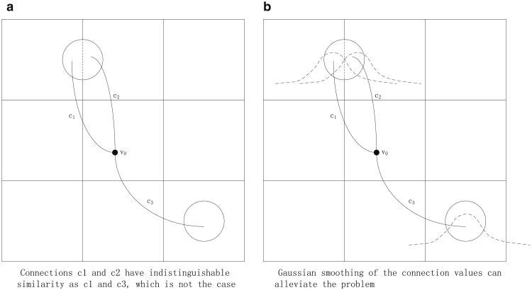
The most accurate representation of a connectivity profile of a voxel is a complete list of the numbers of connections to all voxels. However this representation has very high computational complexity for computing profile similarity between voxels, and hence it is practical only if each structure has relatively few connections. This is not the case for probabilistic tractography, in which many voxels project streamlines to many other voxels. In our framework, we construct a voxel's connectivity profile by first coarsening the spatial resolution of the volume (each coarse cell consists of 4 × 4 × 4 voxels), and then counting the number of connections from a voxel to each of these coarser cells. This substantially reduces the computational and storage costs, and increases the SNR so that more robust results can be achieved. The connectivity profile of a specific voxel is then defined as these connection values organized as a vector (c1, c2, …, cn)T, where ci is the number of connections from the voxel to cell i, for all the coarse cells. This formulation may cause the so-called “cross-cell” artifact (Fig. 2), in which two connections that are close to each other may be distributed to different cells, and therefore may appear very different from the perspective of the vector-based metric. To alleviate such artifacts, we employ Gaussian smoothing on the connectivity profile vectors. Note that the coarsened cells are all located exclusively in gray matter, and that there are approximately 2,000 such coarsened cells for each subject.
Fig. 2. “Cross-cell” artifact.
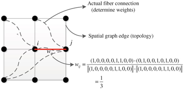
In order to integrate spatial proximity and to avoid the generation of spurious clusters, we formulate parcellation as a graph-cut problem, where the topology of the graph is independent of the connectivity data. In particular, the topology of the graph is simply a grid that reflects Euclidean spatial proximity. We use connectivity profiles to calculate the edge weights of this graph; thus, a higher edge weight reflects a greater similarity between the connectivity profiles of the corresponding voxels. Figure 3 illustrates this representation. In Fig. 3, solid lines represent the edges in the graph, and dashed lines are the physical connections as determined by the tractography algorithm. The weight of an edge (solid line) is a function of the similarity of the connectivity profiles of its two terminal nodes. As in Fig. 3, if the cosine similarity metric is used, wij is simply the cosine of the connectivity profile vectors corresponding to voxels i and j. From this perspective, our goal is to partition the graph into K connected subgraphs, such that the total weights of the links whose terminals are in different subgraphs are minimized subject to constraints on the subgraphs. In practice, we can choose K based on based on domain expertise, or according to stability analysis of the clustering algorithm (Levine and Domany 2001). In our framework, we choose K to be equal to 90 to comply with AAL-90 atlas region definitions, in order to facilitate comparison of the resulting atlas with the AAL-90 atlas.
Fig. 3. Topology and connection weights of the formulated graph-cut problem.
Multiclass Hopfield Network (MHN)
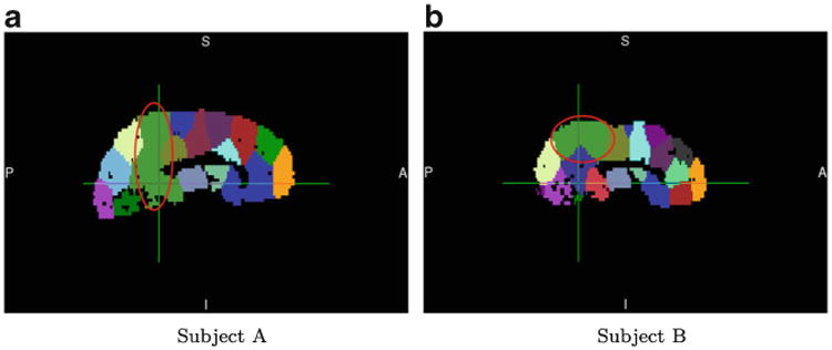
The optimal graph cut problem is NP-complete (Karp 1972). There are many algorithms that approximately solve the graph-cut problem; however, our graph-cut problem is slightly different from the prototype, in that we impose a constraint on the subgraphs (each subgraph must significantly overlap with an AAL region). Generally, the most effective strategy for solving constrained graph-cut problems is spectral clustering, where the constraint results in a balance among the subgraphs, referred to as either ration-cut or normalized-cut (Von Luxburg 2007). Most other clustering algorithms require initialization, and to varying degrees, their results depend on such initialization. This dependence poses a challenge, as we seek consistency of parcellation results across runs, and particularly across subjects, to enable group-level analyses. One possible solution is to enforce a common initialization for all of the subjects. Assuming that the general geometry of brain networks is broadly similar across subjects within an experimental group, a clustering algorithm with common initialization should yield similar results across subjects within the group, thereby rendering these parcellations amenable to group-level analysis. Although spectral clustering would appear to be the most promising solution to our graph-cut problem, the challenge with spectral clustering is that its initialization lies in the k-means stage, where the cluster means of the connectivity profiles, rather than the node labels, are initialized. These cluster means have few degrees of freedom, provide little information about the topology of the spatial-proximity graph, and therefore yield results that manifest different connectivity-based clustering results across runs. For example, Fig. 4 shows parcellation results obtained by using spectral clustering with initial centroids computed from corresponding AAL-90 parcellations, for two subjects from our data set. It is clear from visual inspection that the circled regions have completely different definitions in the two parcellation results.
Fig. 4. Spectral clustering based on cluster-mean initialization results in widely varying region definitions across subjects; subjects A and B were randomly selected from our data set.
To address this problem, we propose a novel clustering algorithm based on a multiclass version of the Hopfield network model (Hopfield 1982). Our multiclass Hopfield network (MHN) algorithm employs a Hopfield network to perform clustering on a graph structure, taking advantage of the natural similarity between the Hopfield network energy function and the clustering objective. MHN modifies the parcellation during each iteration, so as to increase the homogeneity of connectivity metrics within each structure. By initializing this algorithm with cluster labels, rather than cluster centroids, we ensure that region definitions are preserved across subjects.
Hopfield networks were originally proposed to model associative memory. A standard Hopfield network is formulated by a weighted graph, and binary node values (1 or -1). Upon retrieval of stored memory, the update rule converges on the local minimum of the energy function (assuming no nodal bias is introduced):
| (1) |
The optimal solution to this equation will assign opposite labels to terminal nodes of edges with small weights, and the same label to terminal nodes of edges with large weights. Minimizing this function therefore can guide the search for a good graph cut.
The update rule for retrieving a local minimum of the energy is very simple: in each iteration, we first select an arbitrary order for node update, and then apply the following update rule:
| (2) |
Under these conditions, these updates are guaranteed to converge to a local minimum. To generalize the model to accommodate multi-class variables, we modify the energy function and the update rule. In our formulation, the connectivity profile signature of a node is changed to a 1-out-of-k vector denoting cluster affiliation:
| (3) |
where I is the identity function, c is the (current) cluster label of the voxel, and k is the total number of clusters. The energy function now becomes
| (4) |
And the update rule becomes
| (5) |
| (6) |
where yij denotes the jth component of vector yi computed by the above equation. The last equation converts the real-value connectivity profile signature back to the 1-out-of-k vector domain. It is straightforward to prove that a similar convergence theorem holds for our MHN framework; again, the guarantee is for only a local optimum. To mitigate this problem, we employ simulated annealing (Aarts and Korst 1988), which allows the MHN algorithm to explore a larger search space early on, and focus on a smaller fraction of the search space as the annealing schedule progresses. The update rule with simulated annealing is
| (7) |
| (8) |
| (9) |
where ek denotes a vector with only one non-zero entry at position k, T specifies the “temperature” for the cool-down, or annealing, process, and α is a factor in [0, 1] that controls the rate of cooling.
Growing Individual Brain Parcellations
Individual brain parcellations are grown in individual subjects' local diffusion spaces. We used the AAL-90 atlas to initialize parcellation for each subject. We first applied the FSL tool FNIRT to register the atlas (MNI space) to each subject's diffusion space. The AAL-90 atlas consists of 90 structures; we therefore extracted each of the AAL-90 regions as a binary mask and then registered each region to the subject's local diffusion space. We then concatenated the 90 registered masks to form the initialization of the parcellation, i.e., each voxel was represented by a vector with 90 components. We used the default tri-linear interpolation method in FNIRT for performing this registration task, which can result in non-binary values, which MHN keeps intact during initialization. To prevent marked changes from the initial AAL structures, we chose a low initial temperature T(0) for MHN's simulated-annealing component.
The MHN algorithm applied the Hopfield network update rule to each subject's data, for a maximum of 100 iterations. For most of the cases being tested, the update ceased to change within 100 iterations. We converted the resulting 1-out-of-90 label vectors back to value indices (i.e. numerically from 1 to 90, as cluster labels) for visualization and group-level analysis. The result was, for each subject, an individualized atlas in that subject's coordinate space, consisting of 90 structures.
Group Atlases
Individual atlases were registered back to the MNI space; each voxel of these registered individual atlases was represented by a 90-dimensional vector, representing the relative contributions of the original AAL structures to the final atlas structure at that voxel, for that subject. We averaged these individual registered atlases, to obtain a probabilistic group-level MNI-space atlas.
To measure group differences, we require a statistic that is symmetrical, and that reflects the distance between two probability vectors. Rather than test a group-difference hypothesis directly on high-dimensional data, we randomly partitioned the data into groups, and computed a scalar metric reflecting the total difference between the group atlases under that particular grouping. We then computed the two-sample t statistic to determine the significance of the “difference of the difference” between the two grouping protocols.
In summary, the steps for computing and comparing group-level atlases for control and schizophrenia subject are:
For each subject, save each of the 90 atlas structures as a binary image.
Register each of these binary images to the MNI space using FNIRT in FSL, resulting in real-valued (rather than binary) atlas structures.
Combine the 90 registered atlas-structure images for each subject to obtain “atlas likelihood vectors”, where each of the 90 values of the vector corresponding to a voxel measures the likelihood that this voxel belongs to the specific atlas structure for that subject.
Average the atlas likelihood vectors for each group and normalize such that elements of the averaged vectors sum to 1.0, so that we can interpret the vectors as categorical distribution parameters. We then construct the group atlas by assigning each voxel its most probable cluster label. We can also visualize voxel-wise “confidence levels”, meaning the likelihood value of the most probable cluster label, to provide a visual summary regarding which regions have consistent connectivity patterns and which regions do not. In our implementation, the confidence level is visualized simply as the magnitude of the largest entry in the atlas likelihood vector.
Compute the difference between two group atlases. Because of its symmetry and numerical robustness, we choose the squared Hellinger distance (Hellinger 1909) to quantify the difference between two voxels' probability vectors. This metric is preferable to the KL-divergence metric for our purposes because the latter commonly goes out of scale in the presence of a component whose value is close to 1 in one atlas, and close to 0 in the other.
Measure the significance of several grouping protocols. There were three grouping protocols used: (i) schizophrenia (SZ) group vs. normal control (NC) group (SZ-NC); (ii) Two randomly selected groups from the entire dataset (Rand-All); (iii) Two randomly selected groups from the NC group (Rand-NC). For each of the three partitions, we sample 39 subjects in each group for each run, and test each partitioning for 10 runs. Voxel-wise differences in each run are overlaid over each other and displayed in a single graph.
Results
We first note that the MHN parcellation method results in structurally more homogeneous regions compared to AAL structures, in the sense that the voxels within a region have significantly more similar connectivity profiles than those of the AAL regions. Figure 5 compares the average similarity of each MHN region for the NC and SZ groups, relative to the corresponding AAL regions. As can these graphs demonstrate, each MHN region is significantly more homogeneous in terms of the connectivity profiles of its voxels, and hence captures structural connectivity information much more effectively, than the corresponding AAL region.
Fig. 5.
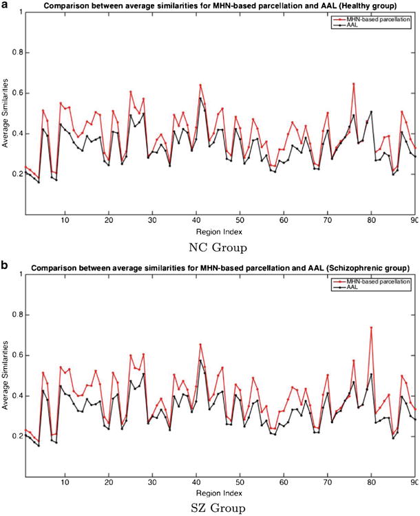
Region Connectivity Profile Similarity for NC and SZ Groups. The Similarity metric used is the average correlation between the connectivity profiles of pairs of voxels within a region
In addition, we performed two analyses to evaluate the merits of the MHN parcellation method. In the first experiment, we computed, for each of the AAL and MHN atlases, the volume for each defined region, the connectivity values between each pair of defined regions, and the two-sample t-test statistics comparing the SZ group with the NC group. In the second experiment, we used these region-volume and connectivity data as features to train support vector machine (SVM) classifiers, and thereby compared classification accuracies across atlases. Note that, in these analyses, changes in atlas-structure volumes are not due to atrophy; rather, they are due to changes in connectivity that lead to re-assignment of region labels for individual voxels.
Visualization of Parcellation Results; Statistical Analysis
Results in this section demonstrate that MHN generates parcellations that are significantly different from the AAL-90 atlas. For this purpose, we apply MHN to the data set described in Section “Data and Preprocessing”. We then compare regional volume differences and connectivity differences based on the two-sample t-test statistic.
Figure 6 shows examples of parcellation results for two subjects: S01 (a SZ subject) and S02 (a NC subject). The figure illustrates consistent differences between the AAL-90 atlas and the connectivity-based atlas. The most common structure-deformation pattern is shown in three regions, circled in red and yellow; this deformation consists of arranging an atlas structure such that its orientation better conforms to subcortical white matter fiber orientation; we call this change “columnization”. Visual comparison qualitatively indicates the volume change in the light green region in the red circle, which corresponds to the t-test results shown as region 27 in Table 1.
Fig. 6. Consistent deviations of MHN parcellations from AAL atlas structures.
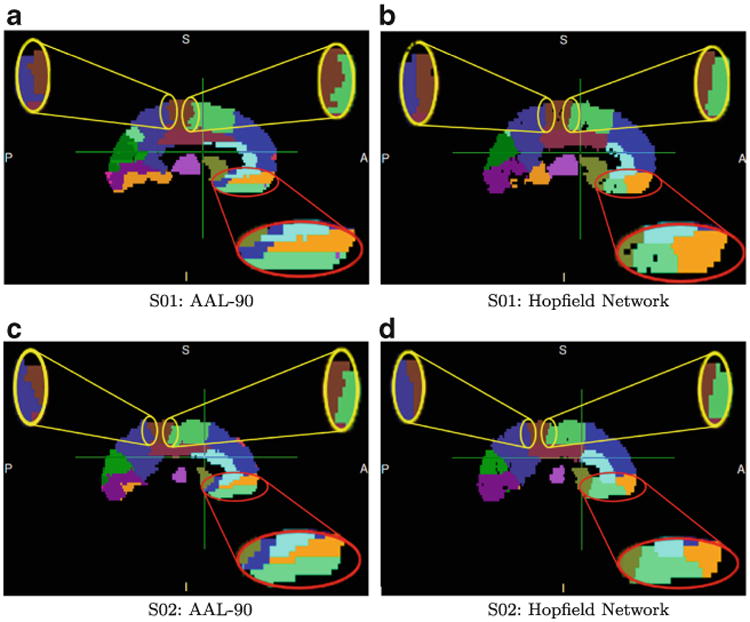
Table 1. Greatest region volume changes detected using MHN.
| Region Name | p-value |
|---|---|
| Temporal_Sup_R | 4.61E-06 |
| Insula_R | 7.54E-06 |
| Rectus_L | 1.05E-04 |
| Cuneus_R | 1.28E-04 |
| Temporal_Mid_R | 5.56E-04 |
| Cuneus_L | 1.97E-03 |
| Calcarine_L | 5.42E-03 |
| Temporal_Mid_L | 5.86E-03 |
| Postcentral_L | 5.89E-03 |
| Frontal_Inf_Tri_L | 7.17E-03 |
| Parietal_Sup_L | 1.23E-02 |
| Cingulum_Ant_L | 1.32E-02 |
| Rectus_R | 1.37E-02 |
| Frontal_Mid_R | 1.52E-02 |
| Parietal_Sup_R | 1.57E-02 |
| Cingulum_Mid_R | 2.70E-02 |
| ParaHippocampal_L | 3.31E-02 |
| Occipital_Mid_R | 3.44E-02 |
| Fusiform_R | 3.58E-02 |
| Cingulum_Ant_R | 4.12E-02 |
| Temporal_Sup_L | 4.79E-02 |
| Occipital_Mid_L | 4.97E-02 |
| Frontal_Inf_Orb_R | 5.11E-02 |
To obtain insights regarding group differences in their corresponding atlas structures, we tested the hypothesis that a MHN region differed significantly between experimental groups. In the first experiment we counted, for each atlas structure, the number of voxels in each region across each group and then computed the two-sample t statistic to determine the significance of volume changes between the two groups. Since we used AAL-90 regions as our initialization, and our implementation of the Hopfield network procedure allowed only incremental changes to these regions, we retained structure names for the resulting regions. The regions having the lowest p-values are shown in Table 1. Region volumes are normalized by individual total brain volumes before computing p-values.
The t-test results indicate the significance of atlas changes. Based on the MHN-derived atlas, we can also measure connectivity changes between atlas structures. The connectivity value between two regions is defined as the total number of sampled connections obtained via PROBTRACTX between any pair of voxels from the two regions. The t-statistic measures the significance of change for each of the 4005 connection values. Part of the results are shown in Table 2.
Table 2. Greatest connectivity changes detected using MHN.
| Region 1 | Region 2 | p-value |
|---|---|---|
| Precentral_R | Cingulum_Post_R | 7.14E-06 |
| Precentral_R | Cingulum_Post_L | 1.65E-05 |
| Cingulum_Mid_L | Cingulum_Mid_R | 1.76E-05 |
| Postcentral_L | Thalamus_L | 3.58E-05 |
| Frontal_Mid_L | Frontal_Inf_Tri_L | 4.29E-05 |
| Cuneus_R | Precuneus_R | 1.03E-04 |
| Cingulum_Mid_R | Putamen_L | 1.08E-04 |
| Temporal_Sup_L | Temporal_Mid_L | 1.28E-04 |
| Supp_Motor_Area_L | Cingulum_Post_R | 1.36E-04 |
| Supp_Motor_Area_L | Parietal_Sup_L | 1.53E-04 |
| Supp_Motor_Area_R | Cingulum_Mid_R | 1.57E-04 |
| Precentral_L | Thalamus_R | 2.07E-04 |
| Frontal_Sup_Medial_L | Parietal_Sup_L | 2.18E-04 |
| Frontal_Inf_Tri_L | Rectus_L | 2.34E-04 |
| Frontal_Mid_R | Supp_Motor_Area_L | 2.39E-04 |
| Supp_Motor_Area_L | Angular_R | 2.46E-04 |
| Rectus_L | Cingulum_Post_L | 2.59E-04 |
| Cingulum_Mid_R | Hippocampus_L | 2.67E-04 |
| Precentral_R | Cingulum_Mid_L | 2.69E-04 |
| Insula_L | Temporal_Sup_L | 3.13E-04 |
| Insula_R | Thalamus_R | 3.15E-04 |
| Supp_Motor_Area_L | Temporal_Mid_R | 3.27E-04 |
| Rolandic_Oper_L | Temporal_Sup_L | 3.92E-04 |
Classification Accuracy
In addition to directly comparing group-averaged parameters between the atlas structures, we also used these atlases to generate classifiers to distinguish the NC from SZ subjects. To the extent that our atlas generation procedure delineates connectivity patterns that truly differ between the NC and SZ groups, classifiers constructed using our atlas-based variables should be more accurate than those using structures from the original AAL atlas.
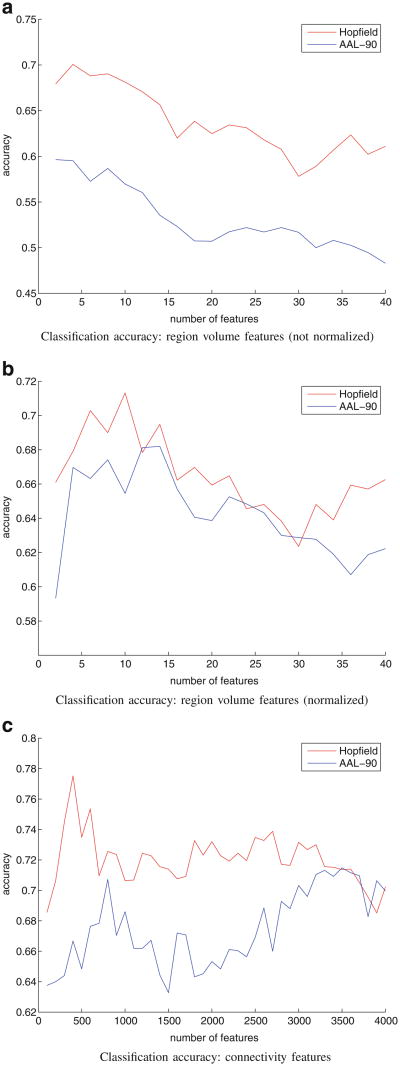
We generated classifiers based both on volume features and connectivity features derived from both atlases. Regional volume features and connectivity features were the same parameters used in Section “Visualization of Parcellation Results; Statistical Analysis”. For regional-volume features, we tested both normalized (to total brain volume) and non-normalized atlas structures. For the MHN classifier, we included features in order of their p-value rankings in Tables 1 and 2. For the AAL-based classifier, we included features in order of their p-values obtained from the AAL structures of the two groups. In each cross-validation experiment, we ran 100 trials, and in each trial we randomly sampled approximately 3/4 of the entire data set to generate a training set (including NC and SZ groups) for constructing a linear SVM, and used the remaining 1/4 as a test set. We recorded mean classification accuracy across the 100 trials for each experiment.
Figure 7 displays classification results based on region volume features and connectivity features, with the number of region volume features in a particular experiment ranging from 2 to 40 out of 90 possible regions, and connectivity features ranging from 100 to 4,000 out of 4,005 potential connections. To demonstrate that the MHN algorithm indeed generates better parcellations, we performed the same classification experiment with parcellations that are solely AAL-90 atlas registered onto individual diffusion spaces (a separate t-test analysis is conducted to determine the feature inclusion order for AAL-90 features, which is different from the MHN case). These graphs demonstrate that MHN parcellations distinguish schizophrenic from non-schizophrenic subjects much more accurately than the original AAL-90 atlas structures from which they were derived.
Fig. 7. Classification accuracy.
Group-Level Atlas Differences
This section describes test results regarding group atlas generation. The goal is to demonstrate that MHN yields systematic atlas changes across groups. Figure 8 shows the atlas resulting from averaging across all SZ subjects, and the corresponding confidence level for each voxel. Figure 9 shows the corresponding images for the NC group. Figure 10 displays the voxel-wise difference between the two groups. For example, the bright voxel at the cross-hairs in this Figure indicates that the cluster-label distribution differs greatly between the two group atlases at that location. This voxel is near the boundary of the right Superior Temporal Gyrus, which is the region that manifested the most significant volume change as measured by our two-sample t statistic.
Fig. 8.
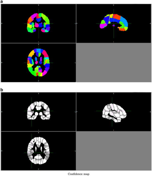
Group atlas of the schizophrenic group. A = anterior, P = posterior, R = right, L = Left, I = inferior, S = superior
Fig. 9.
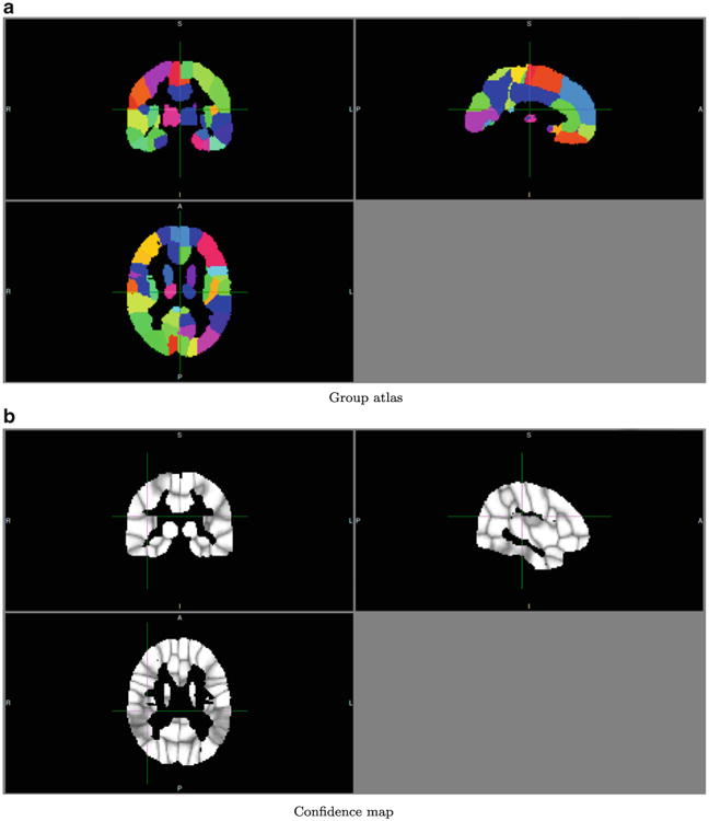
Group atlas of the control group. A = anterior, P = posterior, R = right, L = Left, I = inferior, S = superior
Fig. 10.
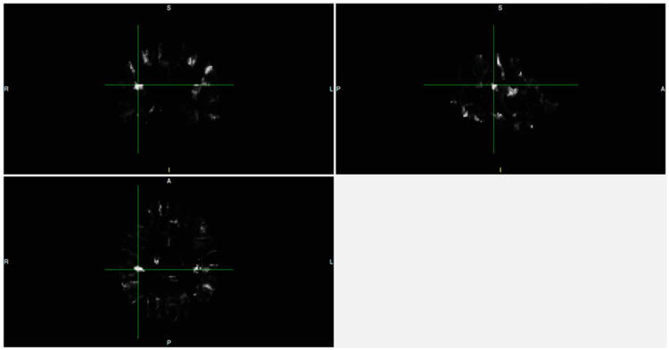
Difference map between two group atlases. A = anterior, P = posterior, R = right, L = Left, I = inferior, S = superior
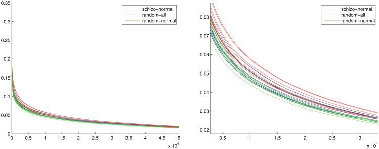
Figure 11 shows the distribution of voxel-wise differences between several random grouping protocols. The difference values are arranged in the descending order of voxel difference values. The right figure is a zoomed-in local view of the left figure.
Fig. 11. Voxel-wise group difference distributions.
As described in Section “Group Atlases”, we computed two-sample t statistics to test the significance of the “difference of difference” for each grouping protocol. In this experiment, we randomly generated 10 groupings for each grouping protocol, i.e., in each instance of a grouping protocol, we randomly sampled 39 subjects (without replacement) for each group according to the grouping protocol, and for each grouping protocol we repeated this procedure 10 times. We generated a pair of group atlases for each instance. The p-value for the total difference between the SZ-NC partition and the Rand-All partition was 0.0016, and the p-value between SZ-NC partition and the Rand-NC partition was 3.33E-5. These results imply that the SZ-group atlas has significant systematic connectivity differences relative to the NC-group atlas. This also shows that the SZ-group atlas manifests greater variance in its connectivity patterns, relative to the NC-group atlas.
Discussion
We have described a novel data-driven, connectivity-based atlas-generation algorithm. Our preliminary evaluation indicates that our approach can yield consistent connectivity-based parcellation patterns among subjects within an experimental group, and that these patterns differ from those of AAL-90 atlas structures, as shown in Fig. 6. These differences include re-configuration of some of the standard regions (an example is shown in the red circle in this Figure), and the “columnization” effect shown in the yellow circles.
To place the atlas structures generated by MHN in a clinical context, we compared region volumes and inter-structure connectivity patterns resulting from our parcellation method. The regions manifesting greatest change in the MHN atlas are consistent with previous reports in the schizophrenia literature (Honea et al. 2005). In addition, our classification experiments confirmed that connectivity-based atlas structures yield classifiers that more accurately distinguish schizophrenic from control subjects with greater accuracy than do AAL structures (78 % versus 71 % maximal accuracy).
We applied a simple registration and averaging scheme to obtain group-level atlases in the MNI space. Averaging removes many individual variations, and thus results in more regular shapes. The information about individual variations is preserved in confidence-map visualization, from which we can readily tell which regions have relatively consistent connectivity patterns. For example in Fig. 9b, the left superior temporal gyrus, right superior temporal gyrus, left middle temporal gyrus, and right middle temporal gyrus have lower confidence values, indicating lack of consistency of superior/middle temporal regions in terms of their connectivity patterns.
Figure 11 illustrates the fact that there are significant group differences between SZ and NC subjects that are very unlikely to be explained by chance, as determined by the two-sample t-test. The fact that the SZ-NC vs. Rand All comparison yields a larger p-value than the SZ-NC vs. Rand-NC comparison indicates that the Rand-All group has larger variance than the Rand-NC group, which in turn indicates that the SZ group has relatively greater variance in connectivity patterns.
Finally, there are six main future directions for extending this approach. First, although our method integrates connectivity information into atlas parcellation, our initial implementation of MHN anchored on initialization values, and therefore this implementation is not completely data driven. Furthermore, as indicated in Fig. 4, the AAL-90 atlas does not conform to connectivity patterns, and therefore is not the optimal initialization for connectivity-based voxel clustering. To be able to build a connectivity based atlas without relying on a pre-defined initialization, we will need to solve the problem of properly registering connectivity data to a standard space, so that we can directly average connectivity data across subjects. Second, being able to average connectivity data directly in a standard space, rather than doing so based on registration of atlas structures, would increase the accuracy of our approach. Third, we plan to reimplement MHN to exploit the inherent parallel nature of the preprocessing and clustering components; this extension will allow us to compare large numbers of different initializations, including random and other non-atlas initializations, to gauge convergence properties, to determine the relative performance of different parcellation approaches, and will also allow us to increase spatial resolution. Fourth, we plan to evaluate methods for automatically determining the optimal number of atlas structures, for example based on minimum description length or other entropy-based metrics. Fifth, we plan to explore additional clustering approaches, with an emphasis on scalability. Finally, we must extend our initial evaluation beyond the single data set and atlas presented here. Toward this end, we plan to evaluate MHN using DTI data from normal subjects, as well as subjects with disorders known to be at least partially due to altered connectivity, such as autism spectrum disorder and schizophrenia. For the latter, we will extend the sample we acquired for initial evaluation of the MHN approach. Such evaluation is critical to determining the generalizability, scalability and accuracy of our approach.
Conclusion
Many atlas-based connectivity analyses employ atlases whose parcellations are based on histological or mesoscopic anatomic features. To provide a source of connectivity-derived atlases, we have implemented a novel whole-brain parcellation method based on anatomical connectivity information. Our method recasts brain parcellation as a graph-cut problem on a sparse graph; this approach simultaneously captures spatial closeness and connectivity information. The graph-cut problem is solved using a novel multi-class Hop-field network algorithm, in combination with simulated annealing. Our implementation is computationally efficient, and converges very quickly. We have applied our method to data from an ongoing schizophrenia study. We found that our connectivity-based atlas resulted in connectivity-based parcellation patterns that were consistent among subjects within an experimental group; as expected. In addition, the resulting atlas structures had more consistent connectivity patterns than standard atlas structures. In addition, we achieved more accurate classification of schizophrenia and control subjects using our connectivity-based atlas. Finally, we found that regions exhibiting the greatest differences between the two groups have been described previously in the schizophrenia literature.
Acknowledgments
This work was supported by the National Institutes of Health (R01MH085646, P50MH103222, and R01DA027680 to LEH) and by the University of Maryland's Center for Health Informatics and Bioimaging, and the State of Maryland MPower initiative (to EHH and JJ).
Footnotes
Information Sharing Statement: Both the source code and documentation are available on request.
Contributor Information
Qi Wang, Email: qiwang321@gmail.com.
Joseph JaJa, Email: joseph@umiacs.umd.edu.
Yu Jin, Email: yuj@umd.edu.
References
- Aarts E, Korst J. Simulated annealing and boltzmann machines: a stochastic approach to combinatorial optimization and neural computing 1988 [Google Scholar]
- Amunts K, Kedo O, Kindler M, Pieperhoff P, Mohlberg H, Shah N, Habel U, Schneider F, Zilles K. Cytoarchitectonic mapping of the human amygdala, hippocampal region and entorhinal cortex: intersubject variability and probability maps. Anatomy and Embryology. 2005;210(5–6):343–352. doi: 10.1007/s00429-005-0025-5. [DOI] [PubMed] [Google Scholar]
- Beckmann CF, DeLuca M, Devlin JT, Smith SM. Investigations into resting-state connectivity using independent component analysis. Philosophical Transactions of the Royal Society B: Biological Sciences. 2005;360(1457):1001–1013. doi: 10.1098/rstb.2005.1634. [DOI] [PMC free article] [PubMed] [Google Scholar]
- Behrens T, Berg HJ, Jbabdi S, Rushworth M, Woolrich M. Probabilistic diffusion tractography with multiple fibre orientations: What can we gain? Neuroimage. 2007;34(1):144–155. doi: 10.1016/j.neuroimage.2006.09.018. [DOI] [PMC free article] [PubMed] [Google Scholar]
- Belmonte MK, Allen G, Beckel-Mitchener A, Boulanger LM, Carper RA, Webb SJ. Autism and abnormal development of brain connectivity. The Journal of Neuroscience. 2004;24(42):9228–9231. doi: 10.1523/JNEUROSCI.3340-04.2004. [DOI] [PMC free article] [PubMed] [Google Scholar]
- Buchanan CR, Pernet CR, Gorgolewski KJ, Storkey AJ, Bastin ME. Test–retest reliability of structural brain networks from diffusion mri. Neuroimage. 2014;86:231–243. doi: 10.1016/j.neuroimage.2013.09.054. [DOI] [PubMed] [Google Scholar]
- Bullmore E, Sporns O. Complex brain networks: graph theoretical analysis of structural and functional systems. Nature Reviews Neuroscience. 2009;10(3):186–198. doi: 10.1038/nrn2575. [DOI] [PubMed] [Google Scholar]
- Bullmore E, Sporns O. The economy of brain network organization. Nature Reviews Neuroscience. 2012;13(5):336–349. doi: 10.1038/nrn3214. [DOI] [PubMed] [Google Scholar]
- Cloutman LL, Ralph MAL. Connectivity-based structural and functional parcellation of the human cortex using diffusion imaging and tractography. Frontiers in Neuroanatomy. 2012;6 doi: 10.3389/fnana.2012.00034. [DOI] [PMC free article] [PubMed] [Google Scholar]
- Collins DL, Holmes CJ, Peters TM, Evans AC. Automatic 3-d model-based neuroanatomical segmentation. Human Brain Mapping. 1995;3(3):190–208. [Google Scholar]
- Hagmann P, Kurant M, Gigandet X, Thiran P, Wedeen VJ, Meuli R, Thiran JP. Mapping human whole-brain structural networks with diffusion mri. PloS One. 2007;2(7):e597. doi: 10.1371/journal.pone.0000597. [DOI] [PMC free article] [PubMed] [Google Scholar]
- Hayasaka S, Laurienti PJ. Comparison of characteristics between region-and voxel-based network analyses in resting-state fmri data. Neuroimage. 2010;50(2):499–508. doi: 10.1016/j.neuroimage.2009.12.051. [DOI] [PMC free article] [PubMed] [Google Scholar]
- Hellinger E. Neue begründung der theorie quadratischer formen von unendlichvielen veränderlichen. Journal für die reine und angewandte Mathematik. 1909;136:210–271. [Google Scholar]
- van den Heuvel MP, Mandl RC, Kahn RS, Pol H, Hilleke E. Functionally linked resting-state networks reflect the underlying structural connectivity architecture of the human brain. Human Brain Mapping. 2009;30(10):3127–3141. doi: 10.1002/hbm.20737. [DOI] [PMC free article] [PubMed] [Google Scholar]
- Honea R, Crow TJ, Passingham D, Mackay CE. Regional deficits in brain volume in schizophrenia: a meta-analysis of voxel-based morphometry studies. American Journal of Psychiatry. 2005;162(12):2233–2245. doi: 10.1176/appi.ajp.162.12.2233. [DOI] [PubMed] [Google Scholar]
- Hopfield JJ. Neural networks and physical systems with emergent collective computational abilities. Proceedings of the National Academy of Sciences. 1982;79(8):2554–2558. doi: 10.1073/pnas.79.8.2554. [DOI] [PMC free article] [PubMed] [Google Scholar]
- Jenkinson M, Beckmann CF, Behrens TE, Woolrich MW, Smith SM. Fsl Neuroimage. 2012;62(2):782–790. doi: 10.1016/j.neuroimage.2011.09.015. [DOI] [PubMed] [Google Scholar]
- Karp RM. Reducibility among combinatorial problems. Springer; 1972. [Google Scholar]
- Kötter R, Hilgetag CC, Stephan KE. Connectional characteristics of areas in walker's map of primate prefrontal cortex. Neurocomputing. 2001;38:741–746. [Google Scholar]
- Levine E, Domany E. Resampling method for unsupervised estimation of cluster validity. Neural Computation. 2001;13(11):2573–2593. doi: 10.1162/089976601753196030. [DOI] [PubMed] [Google Scholar]
- Mori S, Wakana S, Van Zijl PC, Nagae-Poetscher L. Mri atlas of human white matter. 2005 doi: 10.1148/radiol.2301021640. [DOI] [PubMed] [Google Scholar]
- Nanetti L, Cerliani L, Gazzola V, Renken R, Keysers C. Group analyses of connectivity-based cortical parcellation using repeated < i> k-means clustering. Neuroimage. 2009;47(4):1666–1677. doi: 10.1016/j.neuroimage.2009.06.014. [DOI] [PubMed] [Google Scholar]
- Passingham RE, Stephan KE, Kötter R. The anatomical basis of functional localization in the cortex. Nature Reviews Neuroscience. 2002;3(8):606–616. doi: 10.1038/nrn893. [DOI] [PubMed] [Google Scholar]
- Roca P, Rivière D, Guevara P, Poupon C, Mangin JF. Medical image computing and computer-assisted intervention–MICCAI 2009. Springer; 2009. Tractography-based parcellation of the cortex using a spatially-informed dimension reduction of the connectivity matrix; pp. 935–942. [DOI] [PubMed] [Google Scholar]
- Roca P, Tucholka A, Rivière D, Guevara P, Poupon C, Mangin JF. Medical image computing and computer-assisted intervention–MICCAI 2010. Springer; 2010. Inter-subject connectivity-based parcellation of a patch of cerebral cortex; pp. 347–354. [DOI] [PubMed] [Google Scholar]
- Supekar K, Menon V, Rubin D, Musen M, Greicius MD. Network analysis of intrinsic functional brain connectivity in alzheimer's disease. PLoS Computational Biology. 2008;4(6):e1000,100. doi: 10.1371/journal.pcbi.1000100. [DOI] [PMC free article] [PubMed] [Google Scholar]
- Tzourio-Mazoyer N, Landeau B, Papathanassiou D, Crivello F, Etard O, Delcroix N, Mazoyer B, Joliot M. Automated anatomical labeling of activations in spm using a macroscopic anatomical parcellation of the mni mri single-subject brain. Neuroimage. 2002;15(1):273–289. doi: 10.1006/nimg.2001.0978. [DOI] [PubMed] [Google Scholar]
- Varshney LR, Chen BL, Paniagua E, Hall DH, Chklovskii DB. Structural properties of the caenorhabditis elegans neuronal network. PLoS Computational Biology. 2011;7(2):e1001,066. doi: 10.1371/journal.pcbi.1001066. [DOI] [PMC free article] [PubMed] [Google Scholar]
- Von Luxburg U. A tutorial on spectral clustering. Statistics and Computing. 2007;17(4):395–416. [Google Scholar]
- Zalesky A, Fornito A, Harding IH, Cocchi L, Yücel M, Pantelis C, Bullmore ET. Whole-brain anatomical networks: does the choice of nodes matter? Neuroimage. 2010;50(3):970–983. doi: 10.1016/j.neuroimage.2009.12.027. [DOI] [PubMed] [Google Scholar]
- Zang Y, Jiang T, Lu Y, He Y, Tian L. Regional homogeneity approach to fmri data analysis. Neuroimage. 2004;22(1):394–400. doi: 10.1016/j.neuroimage.2003.12.030. [DOI] [PubMed] [Google Scholar]


