High density 3D printed microfluidic valves, pumps, and multiplexers

Abstract

In this paper we demonstrate that 3D printing with a Digital Light Processor stereolithographic (DLP-SLA) 3D printer can be used to create high density microfluidic devices with active components such as valves and pumps. Leveraging our previous work on optical formulation of inexpensive resins (RSC Adv. 5, 106621, 2015), we demonstrate valves with only 10% of the volume of our original 3D printed valves (Biomicrofluidics 9, 016501, 2015), which were already the smallest that have been reported. Moreover, we show that inclusion of a thermal initiator in the resin formulation along with a post-print bake can dramatically improve the durability of 3D printed valves up to 1 million actuations. Using two valves and a valve-like displacement chamber (DC), we also create compact 3D printed pumps. With 5-phase actuation and a 15 ms phase interval, we obtain pump flow rates as high as 40 μL/min. We also characterize maximum pump back pressure (i.e., maximum pressure the pump can work against), maximum flow rate (flow rate when there is zero back pressure), and flow rate as a function of the height of the pump outlet. We further demonstrate combining 5 valves and one DC to create a 3-to-2 multiplexer with integrated pump. In addition to serial multiplexing, we also show that the device can operate as a mixer. Importantly, we illustrate the rapid fabrication and test cycles that 3D printing makes possible by implementing a new multiplexer design to improve mixing, and fabricate and test it within one day.

Graphical Abstract

In this paper we demonstrate that 3D printing with a Digital Light Processor stereolithographic (DLP-SLA) 3D printer can be used to create high density microfluidic devices with active components such as valves and pumps in a very compact format Valve volume is reduced by a factor of 10, and we demonstrate 1 million valve actuations enabled by adding a thermal initiator to our low-cost, custom resin formulation and a short post-print bake. We show pump flow rates up to 40 microliters/min, and demonstrate a very compact 3-to-2 multiplexer that also functions as a mixer. In addition, we illustrate the rapid redesign-fabrication-test iteration cycle enabled by 3D printing by modifying the multiplexer to improve mixing performance. The turn-around time is just one day to go from the original design to an experimentally tested improved design. The results reported in the paper are a large step forward in demonstrating the promise of 3D printing for microfluidics.

1 Introduction

As we observed in Ref. 1, 3D printing offers a true rapid-prototyping capability for microfluidics in which a “fail fast and often” strategy can be employed to positively disrupt the microfluidic device development process by using early and rapid empirical feedback to iteratively guide and accelerate device development. A key enabler of rapid iteration is fast 3D printing and post-processing such that one or more iterations of fabrication → test → adjust design can be performed in a single day. In addition to a vastly streamlined fabrication process, 3D printing avoids the significant startup and operational costs of a cleanroom, thereby making microfluidic device development available to a much broader audience. Moreover, use of standardized elements and functional blocks in the design and layout of a device can permit non-specialists to apply microfluidics to research, prototyping, and product development in many fields. In our judgment, these factors are indicative of the exceptional potential 3D printing offers ^2–4 to effect a step-change in the trajectory of microfluidics usage similar to the transition in the late 1990’s from glass and silicon microfluidics to soft lithography⁵ using polydimethylsiloxane (PDMS).^6,7

Despite this attractive vision for a much expanded microfluidics community, a number of misconceptions and deficiencies stand in the way of its fulfillment. For example, as we discussed in Ref. 8, microfluidic devices consist of a series of small interconnected voids within a bulk material, and traditional commercial 3D printing tools and resins are not optimized for fabrication of such structures. We demonstrated that with proper formulation of resin optical properties, flow channels with cross sections as small as 60 μm × 108 μm could be reliably fabricated with a commercial digital light processing stereolithographic (DLP-SLA) 3D printer. The resin optical properties primarily affect the vertical (out-of-plane) build resolution, while the DLP pixel pitch and optical imaging system are the critical factors for in-plane resolution.

There is a common misperception that the manufacturer-specified 3D printer resolution represents the achievable void feature size that can be fabricated with the printer. However, as we showed in Ref. 8, this is not the case. The minimum void height is determined by the optical absorption of the resin (we found experimentally that it is ~3.5–5.5h_a where h_a is the inverse of the resin absorption coefficient), while the minimum reliable lateral dimension is 4 times the pixel pitch in the build plane. Nonetheless, some impressive work has been done with commercially available 3D printing tools and materials, including reactionware devices, ^9,10 snap-together discrete microfluidic elements, ¹¹ a continuous nitrate-monitoring device for water contamination, ¹² mail-order microfluidics using a commercial service bureau,¹³ active devices (valves and pumps),¹⁴ and microfluidic circuitry (analogous to electronic circuitry). ¹⁵ The primary disadvantages of these approaches to date is the relatively large minimum void size and consequent overall device size.

In this paper we show significant miniaturization of 3D printed microfluidic devices with integrated valves and pumps based on our previous resin formulation work⁸ and our demonstration of the first reported 3D printed valves. ¹ Specifically, we show how to use a DLP-SLA 3D printer with our inexpensive custom resin formulation to fabricate robust membrane valves 40 pixels in diameter (1.08 mm) with a minimum chamber height of 60 μm. These valves are only 10% the volume of our previous 3D printed valves, ¹ and we have improved their durability from 800 actuations to 1 million actuations. To achieve such durability, we modify the resin composition by adding a thermal initiator such that a post-printing 30 minute oven cure drives further polymerization of the material to create a greater degree of cross linking and mechanical toughness. We then demonstrate a simple pump structure consisting of two valves and one displacement chamber (DC), and experimentally characterize its maximum back pressure and maximum flow rate. Finally, we combine 5 valves and one DC into a compact 3-to-2 multiplexer with integrated pump, utilizing the flexibility of 3D printing to densely arrange device elements within the 3D volume of the device. We also show that the multiplexer can be used as a mixer and that its mixing efficiency can be improved by increasing the number of inlets in the DC.

2 Experimental

2.1 Materials

Our resin formulations consist of monomer, photoinitiator, and absorber, which for this work are poly(ethylene glycol) diacrylate (PEGDA, MW 258), Sudan I, and Irgracure 819, respectively. ^1,16,17 We also include a thermal initiator, azobisisobutyronitrile (AIBN), for post-print thermal curing, the details of which are discussed in Sect. 3.1. It is important to note that use of a low molecular weight PEGDA results in excellent water stability for fabricated parts, ¹⁶ with no swelling or degradation in mechanical strength. PEGDA, Sudan I, and AIBN are obtained from Sigma-Aldrich (St. Louis, MO), and Irgacure 819 from BASF (Vandalia, Illinois). Each is used as received.

The specific resin formulation employed for the work reported in this paper is the 0.4% Sudan I resin discussed in Ref. 8. It is prepared by mixing 0.4% (w/w) Sudan I, 1% (w/w) Irgacure 819, and 0.01% (w/w) AIBN with PEGDA, and sonicating for 30 minutes. The resin is stored in an amber glass bottle wrapped in aluminum foil to protect it from light exposure.

2.2 3D printer

We use an Asiga Pico Plus 27 DLP-SLA 3D printer as described in Ref. 8, which has an LED peak wavelength of 412 nm and an in-plane resolution (pixel pitch) of 27 μm. Microfluidic devices in an individual print run are fabricated on a glass slide (25 mm × 37.5 mm × 1.2 mm) which is attached to the printer build table with double-sided tape. We experienced no issues with the slide damaging the teflon film comprising the bottom of the resin tray as long as we followed the 3D printer manufacturer’s build table alignment procedure. Each slide is prepared by cleaning with acetone and isopropyl alcohol (IPA), followed by immersion in 2% 3-(trimethoxysilyl) propyl methacrylate in toluene for 2 hours. After silane deposition slides are kept in toluene until use.

There are two reasons we use glass slides. The first is that they avoid the need to fabricate the first device layer on the rough (anodized Al) surface of the 3D printer build table, which, especially for resins with high optical absorbance, requires a significantly longer exposure time for the first layer to attach to the build table. Long exposure times deplete the available binding sites on the surface of the layer, making attachment of the next layer problematic. The second reason is that the smooth surfaces of the glass slide offer convenient optical access to observe the interior components of the microfluidic device.

2.3 Device fabrication

Our build layer thickness, l, is 10 μm, which results in a normalized layer thickness, ζ = l/h_a, of 0.57 for the 0.4% Sudan I resin. This is well within the optimal build thickness range we established in Ref. 8.

The key active component in our devices is a membrane valve, the structure of which is shown in Fig. 1a.¹ The valve consists of a 20 μm thick membrane (i.e., 2 build layers) sandwiched between two cylindrical voids which comprise a control chamber (100 μm high) and a fluid chamber (60 μm high), each 40 pixels (1.08 mm) in diameter. The corresponding dimensions of our original 3D printed valves are 50 μm membrane thickness, with 250 μm control chamber and 250 μm fluid chamber heights, both of which are 2 mm in diameter. ¹ The valves in this paper are only 10% of the volume of the valves in our original paper (0.165 mm³ compared to 1.73 mm³). The valves in our original paper were fabricated with a different DLP-SLA 3D printer (B9 Creator) prior to developing our quantitative approach to resin formulation.⁸

Fig. 1.

(CAD design of (a) for a 3D printed membrane valve. Schematic illustration and microscope photos of (b), (d) open and (c), (e) closed valves. The microscope photos show the bottom of the valve. See text for details.

When no pressure is applied to the control chamber (as illustrated in Fig. 1b), the valve is open and fluid can flow between the two channels at the bottom of the fluid chamber. A photomicrograph of an open valve is shown in Fig. 1d. The lighting makes it easy to see the pixelation of the bottom surface of the fluid chamber. The measured surface roughness for horizontal surfaces fabricated with 0.4% Sudan I resin is 0.5 μm with a length scale the size of the pixel pitch. As shown in Fig. 1c, when pressure is applied to the control chamber the membrane deflects downward and seals the fluid channels. The central circular region in which the membrane contacts the bottom of the fluid chamber can be clearly seen in Fig. 1e.

In our devices valves are connected with flow channels that are 150 um high and 6 pixels (162 μm) wide. Although smaller channels can be fabricated with 0.4% Sudan I resin, ⁸ we chose this somewhat larger size to ensure easy, high yield fabrication, even for flow channels as long as 118 mm (for a design that is not included in this paper). Consequently, we never had a problem with flow channel fabrication for the devices discussed in subsequent sections.

After 3D printing, unpolymerized resin must be flushed from the interiors of microfluidic structures. An advantage of our PEGDA resin formulations is that they are low viscosity (57 cP), ⁸ making flushing much easier than for many commercial resins that have significantly higher viscosity. As shown in Ref. 8, the difficulty of flushing unpolymerized resin can be the limiting factor in determining the minimum achievable void size for commercial resins, rather than the actual optical properties of the resin.

Immediately after 3D printing is completed, the sample is removed from the build table and soaked in IPA for 2–3 minutes to dissolve much of the unpolymerized resin. The control and fluid chambers are then carefully flushed with IPA, following which vacuum is applied to extract residual IPA from microfluidic structures. Note that the control chamber design in Fig. 1a has a second channel specifically to permit flushing unpolymerized resin.

Next, we bake the device at 80°C for 30 minutes to activate the thermal initiator to drive further polymerization. It should be noted that a blanket UV exposure is completely ineffective at curing our 3D printed devices because the UV light only penetrates a small fraction of a millimeter even after many hours of exposure due to the high absorption of the resin.

After baking, a device is prepared for testing by inserting Microbore PTFE tubing (0.022″ID × 0.042″OD) into corresponding cylindrical holes in the device (Fig. S1, ESI^†), and gluing the tubing in place (Loctite Instant Mix 5 Minute Epoxy). The epoxy is also used to plug the flushing channels for all control chambers.

Total device build and preparation time is approximately 4 hours, and consists of (1) 3D printing (<1 hour), (2) flushing unpolymerized resin (5–7 minutes for all of the devices in a single print run), (3) oven bake (30 minutes), and (4) inserting tubing followed by mixing and applying epoxy to the junction between the tubing and device and letting the epoxy cure for 2 hours. Despite being labelled as 5 minute epoxy, we found that a 2 hour cure time was needed for the epoxy to achieve a hardness that facilitated leak-tight seals and good tubing strain relief. The epoxy cure step is by far the most time-consuming aspect of our current device fabrication and preparation process. This time can be dramatically reduced to just a few minutes by substituting a UV curable adhesive for the 5 minute epoxy, thereby reducing the total device fabrication and preparation time to under 2 hours.

CAD and .stl design files for the valve, pump, and multiplexer reported in this paper are freely available online. ¹⁸

3 Results and discussion

3.1 3D printed valves

To evaluate the performance of 3D printed valves, we first measured the maximum fluid pressure, P_fluid, at which the valve stays closed for a given control pressure, P_control, applied to the membrane to close the valve. Measurement details are discussed in Section S2, ESI^†. The pressure difference, ΔP = P_control−P_fluid, can be interpreted as the minimum pressure required to deflect the membrane enough to just barely close the valve. We therefore expect that ΔP should increase as the fluid chamber height increases or the membrane thickness increases because either change makes it more difficult to deflect the membrane enough to close the valve. This is confirmed in Figs. S2b, ESI^† and S2c, ESI^† which show the corresponding experimental measurements. In Fig. S2b, ESI^†, an increase in ΔP from a little over 2 psi to 4 psi is observed as the fluid chamber height increases from 50 μm to 80 μm because the membrane has to deflect more to close the valve. We experimentally determined that the fabrication yield for valves with a 50 μm chamber height is substantially less than for a 60 μm chamber height, which is nearly 100%. We therefore chose a 60 μm fluid chamber height for the devices reported in this paper. Similarly, as shown in Fig. S2c, ESI^†, the membrane becomes stiffer and requires more pressure to close as its thickness increases from 2 layers (20 μm) to 4 layers (40 μm).

An important criterion for an active fluidic device is its durability. In our original demonstration of 3D printed valves, ¹ the valves typically lasted 800 actuations before the membranes broke. However, we had previously tested similar cleanroom-fabricated valves to 115,000 actuations with no sign of breakage or degradation in their properties. ¹⁷ Following 3D printing and prior to thermal curing, valve membranes in the present study typically lasted only one or two actuations before breaking. We hypothesized that additional polymerization was needed to increase the mechanical robustness of the membranes. However, as detailed in Ref. 8, other constraints prevent trying to achieve this with longer layer exposure times during 3D printing. Hence we added a thermal initiator with a post-print oven bake to drive further polymerization. We tested a variety of bake times at 80°C, and found that they had no effect on pump properties as shown in Fig. S3, ESI^†. A bake time of 30 minutes seemed to offer the best trade-off between mechanically robust membranes, short bake time, and yield.

In our largest yield test, we began with 54 fabricated valves, one of which was found to leak between the flow channels during its first actuation. We later established that such as-built leaks can be avoided by simply increasing the separation between the channels in the bottom of the valve from 4 pixels to 6 pixels. Of the 53 remaining valves, all but one continued working after 10,000 actuations. The one that failed had its membrane break during the first 1,000 actuations. Of the 53 that survived, we tested one to 1 million actuations, after which it still worked. The flow channels and fluid chamber were filled with water during the entire 30 hours it took to run the test.

3.2 3D printed pumps

As shown in Fig. 2a, a pump consists of two valves (V1 and V2) with a valve-like displacement chamber (DC) in between. The difference between a DC and a valve is that the inlet and outlet channels are placed on the edge of the fluid chamber for a DC rather than in the center as for a valve. This prevents the DC from being able to stop flow when actuated. Note also that the DC is oriented upside down compared to the valves. In a valve the fluid chamber is under the membrane whereas in the DC it is on top of the membrane.

Fig. 2.

(a) CAD design of 3D printed pump. C1–C3 connect to external pressure sources. The partially transparent channels are flushing channels for the valve control chambers, which are later sealed with epoxy. (b) Bottom view of a 3D printed pump. See text for details. (c) Side view photograph of 3D printed pump in (b).

Valve actuation is controlled by applying pressure to C1 and C2, whereas DC actuation is controlled with C3. A photo of a pump looking from underneath is shown in Fig. 2b. The DC appears to partially overlap V1 and V2 since they are placed at different heights in the 3D build volume. The undersides of cylindrical holes are also visible for PTFE tubing to connect C1, C2, and C3 to pressure sources, and the inlet and outlet channels to an off-chip fluid source and sink. Figure 2c is a side view photo of a pump showing the fabricated spatial arrangement of the DC and valves, along with their corresponding flow and control channels.

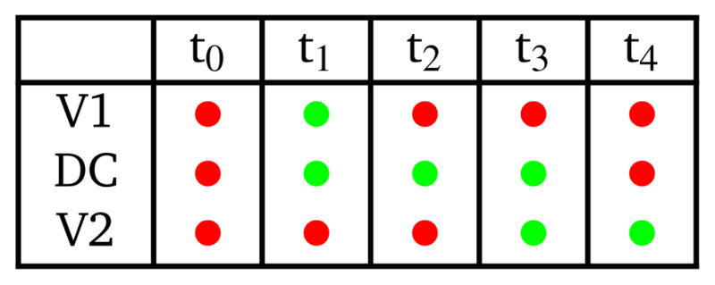
The pump uses a 5-phase cycle as shown in Table 1. At t₀, both valves are closed and pressure is applied to the DC. The DC fluid chamber is therefore in a state of minimum volume. At t₁, V1 opens and the DC pressure is released so the membrane returns to equilibrium thereby pulling fluid through V1 into the DC fluid chamber. At t₂, V1 closes to isolate fluid in the DC from the inlet flow channel, followed by V2 opening at t₃ in preparation for expelling fluid from the DC into the outlet channel, which occurs by actuating the DC at t₄. The cycle then repeats by going back to t₀ in which V1 is closed. The time difference between any two sequential phases is Δt = t_i − t_i−1, which we call the phase interval. Unless otherwise noted, the valve and DC actuation pressure is ~9 psi.

Table 1.

Pump timing logic. Red: actuated (pressure applied; valves closed); green: not actuated (valves open).

A pump’s maximum flow rate, Q_max, for a given set of operating parameters is defined as the flow rate when there is zero back pressure (such as when the fluid source, pump, and fluid outlet are all at the same height). We evaluated Q_max as a function of Δt under two conditions for the unactuated DC control chamber: (1) an applied vacuum of 10 psi (520 mmHg) and (2) vent to atmosphere. In the latter case the restoring force on the membrane is just the elastic strain of the stretched membrane. In the former, an applied vacuum at first assists the elastic strain until the membrane is undeflected and then pulls the membrane up into the control chamber.

The measured maximum flow rate, Q_max, is shown as a function of Δt in Fig. 3a. The maximum flow rate increases as Δt decreases, reaching a peak of 40 μL/min for Δt = 15 ms when vacuum is applied to the DC. The flow rate then drops rapidly as Δt continues to decrease. Note that for Δt ≥ 15 ms, the maximum flow rate with vacuum is approximately twice as large as without vacuum. Calculating the displaced fluid volume as a function of Δt (Fig. 3b), it is apparent that the vacuum pulls the membrane up into the control volume enough to essentially double the volume expelled by the DC for t₃ → t₄ as compared to the no vacuum case. We arbitrarily chose 50 ms (maximum expelled volume) as the phase interval for all subsequent measurements, and used vacuum with the DC.

Fig. 3.

(a) Maximum flow rate (zero back pressure) as a function of the phase interval, Δt. (b) Fluid volume expelled by pump for a single pump cycle calculated from the data in (a). 9 pumps were tested with vacuum and 5 without. The large error bars for vacuum at 20 ms are due to 2 pumps having significantly smaller flow rates than the others. (c) Maximum back pressure as a function of control pressure (average and standard deviation for 7 pumps). (d) Flow rate as a function of the outlet height for a control pressure of 9 psi (average and standard deviation for 6 pumps). Different pumps were used in all tests.

A pump’s maximum back pressure is defined as the maximum pressure the pump can work against such that the flow rate just goes to zero. Measurement details to determine a pump’s maximum back pressure are presented in Section S3, ESI^†, and a typical measurement is shown in Fig. S4, ESI^†. In Fig. 3c, we compare the measured maximum back pressure for control pressures of approximately 6, 9, and 11 psi. A linear curve fit shows an x-intercept of ~4.5 psi, which is the minimum control pressure needed for the pump to be able to push fluid into a zero back pressure outlet. According to Fig. 3c, a control pressure of 9 psi is sufficient to generate a back pressure of approximately 4 psi, whereas a control pressure of 11 psi generates a back pressure of ~8 psi.

In Fig. 3d we measure the flow rate as a function of the height of the outlet above the fluid source and pump. As expected, the flow rate slowly decreases with outlet height. An outlet height of 120 cm corresponds to 1.7 psi of back pressure, in which case the average flow rate decreases from 19.3 μL/min to 17.2 μL/min.

3.3 3D printed multiplexers and mixers

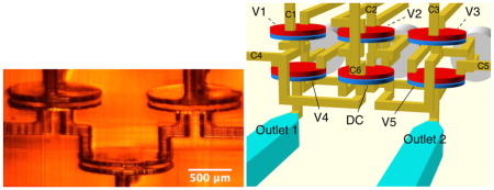
We now use the example of a 3-to-2 multiplexer to illustrate how 3D printing enables high density 3D layout of microfluidic components in a single device. The simplest function of a 3-to-2 multiplexer is to pump fluid from any of three inputs to any of 2 outputs. As discussed in Section 3.2, a pump can be constructed with a DC placed between two valves. Therefore, the smallest component count for a 3-to-2 multiplexer is shown in Fig. 4a where a DC is placed between three input valves (V1, V2, V3) and two outlet valves (V4, V5). Pumping, for example, from Buffer to Outlet 1 uses V1-DC-V4 with all other valves closed. Similarly, pumping from Red to Outlet 2 uses V2-DC-V5. Fluid can be pumped from any of the inlets to any of the outlets by using the associated inlet and outlet valves in conjunction with the DC while keeping all other valves closed. (As a side note, the configuration in Fig. 4a can actually pump fluid from any inlet or outlet to any other inlet or outlet by using the corresponding valves with the DC and appropriate phasing of their actuations.)

Fig. 4.

(a) Multiplexer schematic diagram. (b) CAD design taking advantage of stacked layout flexibility enabled by 3D printing. Valve labeling is the same as (a) with corresponding control lines labeled C1, C2, etc. (c) Bottom view of multiplexer fabricated according to the CAD design in (b). (d)–(i) Demonstration of arbitrary 3-to-2 multiplexing. See text for details. Arrows indicate active flow direction.

One possible 3D layout of the components in Fig. 4a is shown in Fig. 4b in which V1, V2, and V3 are located directly above V4, DC, and V5, respectively. Flow channels and control channels are easily routed through 3D space to form the connections indicated in the schematic diagram in Fig. 4a. The valve, DC, and flow channel dimensions are the same as discussed in previous sections.

A fabricated device is shown in Fig. 4c, looking from below through the glass slide substrate. The valves V1, V2, and V3 are occluded (indicated by dashed white lines) behind V4, DC, and V5 (indicated by solid white lines). PTFE tubing is epoxied in the inlets on the left, and the outlet flow channels are on the right. The three inlet tubes contain buffer (Buffer), diluted red dye in water (Red), and diluted black dye in water (Black), respectively. Both Red and Black have previously been pumped through the device, followed by Buffer. This is the reason the flow channels from the Red and Black inlets to the DC are filled with Red and Black, respectively.

Figures 4d–4i show an example set of operations conducted with the multiplexer that exercise the various combinations of inlets to outlets. It begins with Red being pumped to Outlet 1 (Fig. 4d), followed by Black to Outlet 2 (Fig. 4e), Buffer to Outlet 2 (Fig. 4f), Buffer to Outlet 1 (Fig. 4g), Red to Outlet 2 (Fig. 4h), and Black to Outlet 1 (Fig. 4i). Its dynamic operation is shown in ESI^† Movie S1. During each inlet/outlet combination, the pump is typically run for 50 periods to more than fully flush the previous fluid in the large (500 μm × 500 μm × 2.5 mm) outlet channels. The large outlet channel size is chosen solely to make it easy to see the colored fluids. As a further note, it takes approximately 3 pump periods to flush fluid from the DC when switching from one fluid to another.

The multiplexer can also be used as a mixer by, for example, operating two of the inlet valves simultaneously during pumping, in which case the fluids from the two inlets will be drawn together through the pump and expelled into an outlet. Prior to initiating pump action, we first opened V2, V3, DC, and V5 while raising the reservoirs from which red and black fluid are drawn about 15 cm above the microfluidic device. All of the other valves are closed. Fig. 5a illustrates the gravity-induced flow of Red and Black through the device. The upper right inset shows Black entering the DC from below and Red from above, corresponding to the physical locations of their inlets into the DC. The upper left inset shows the segregated Red/Black flow stream through the DC outlet channel, which maintains its segregation through V5 and Outlet 2 (lower right inset image). Clearly, the only mixing that occurs is due to diffusion across the boundary between the two fluids.

Fig. 5.

(a) Flow generated only by gravity. Note lack of Red/Black mixing. (b, c) Bottom view of DC channel layout in (b) Mixer 1 and (c) Mixer 2. Red channels, R1 in (b) and R1 and R2 in (c), connect the Red inlet valve (V2 in Fig. 4a) to the DC, while the black channels, B1 in (b) and B1 and B2 in (c), connect the Black inlet valve (V3) to the DC. Buffer is the channel that connects the Buffer inlet to the DC through valve V1. O1 and O2 connect the DC to Outlets 1 and 2, respectively, through valves V4 and V5. (d) and (e) compare the mixing performance of the designs in (b) and (c). See text for details.

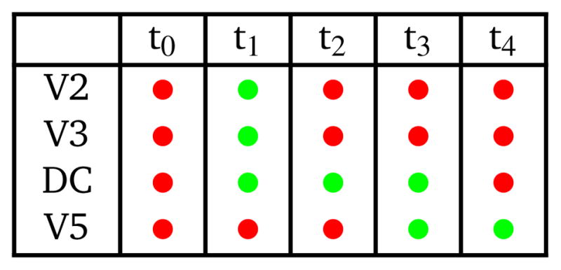
Now consider simultaneous pumping from Red and Black into Outlet 2 according to the timing logic in Table 2. The results are shown in Fig. 5d in which each image shows the device state for the corresponding timing logic in Table 2 (note that t₅ is the same state as t₀). Prior to taking these images, the device was operated long enough such that it had reached a steady-state condition. At t₁ fluid is draw into the DC through open valves V2 and V3, both of which are closed at t₂. The inset for t₂ shows the spatial segregation of fresh Red and Black just drawn into the DC. At t₃ the valve to Outlet 2, V5, is opened, following which fluid is expelled from the DC through V5 into Outlet 2 at t₄. The inset at t₄ shows similar Red/Black segregation in the DC outlet channel, but by the time it makes it through V5 and into Outlet 2 there is much more mixing than in Fig. 5a. However, there is still a discernible red streak near the middle of Outlet 2 (see inset at t₅).

Table 2.

Mixer timing logic. Red: actuated (pressure applied; valves closed); green: not actuated (valves open). Valves not listed in the table are closed.

As soon as we got this result we realized that mixing could be improved by increasing the degree to which Red and Black are interleaved in the DC, which is easily accomplished with a change in geometry. Consider for example the bottom view of the DC in Fig. 5b in which Red is introduced into the DC through flow channel R1, and Black through B1. By splitting each Red and Black inlet into two inlets and interleaving them as shown in Fig. 5c (labeled as R1, R2, B1, and B2), additional mixing can be created in the DC. The mixing properties of the resultant device are shown in Fig. 5e using the same sequence of steps as Fig. 5d. The inset image for t₂ shows red and black regions localized around their respective DC inlets, while the inset at t₄ shows more Red/Black streams in the DC outlet channel, resulting in better mixing in Outlet 2 as seen in the inset at t₅. The rapid iteration time enabled by 3D printing allowed us to redesign, fabricate, and test this new DC inlet design within a day.

As a final comment, the 3-to-2 multiplexer in Fig. 4 can be readily scaled to larger numbers of inlets and outlets. At this point it is unclear what the practical scaling limit is, but it will likely be determined by the fabrication yield of the valves, in which case our fabrication techniques would need to be further refined to increase the valve yield.

4 Summary

In this paper we have demonstrated the potential of 3D printing to enable both rapid fabrication iteration and high density integration of microfluidic components. We have reported the smallest yet 3D printed valves and characterized valve performance and durability. Incorporation of a thermal initiator in the resin together with a post-print bake dramatically improves durability. Fifty two out of 54 valves were successfully tested up to 10,000 actuations, at which point we stopped the tests because of how long they took. One valve was tested to 1 million actuations, after which it still performed well. We have used these valves to create compact pumps and characterized their maximum back pressure and maximum flow rate. Flow rates as high as 40 μL/min have been demonstrated. We have also demonstrated a 3-to-2 multiplexer with integrated pump, and shown that it can also be used as a mixer. Moreover, we have shown the ability to implement and test a new idea to improve mixing within only a day, thereby illustrating the power of 3D printing to enable a “fail fast and often” iterative device development strategy.

References

- 1.Rogers CI, Qaderi K, Woolley AT, Nordin GP. Biomicrofluidics. 2015;9:1–9. doi: 10.1063/1.4905840. [DOI] [PMC free article] [PubMed] [Google Scholar]
- 2.Ho CMB, Ng SH, Li KHH, Yoon YJ. Lab Chip. 2015;15:3627–3637. doi: 10.1039/c5lc00685f. [DOI] [PubMed] [Google Scholar]
- 3.Yazdi AA, Popma A, Wong W, Nguyen T, Pan Y, Xu J. Microfluid Nanofluid. 2016:1–18. [Google Scholar]
- 4.Au AK, Huynh W, Horowitz LF, Folch A. Angew Chem. 2016;128:3926–3946. doi: 10.1002/anie.201504382. [DOI] [PMC free article] [PubMed] [Google Scholar]
- 5.Qin D, Xia Y, Whitesides GM. Adv Mater. 1996;8:917–919. [Google Scholar]
- 6.Duffy DC, McDonald JC, Schueller OJA, Whitesides GM. Anal Chem. 1998;70:4974–4984. doi: 10.1021/ac980656z. [DOI] [PubMed] [Google Scholar]
- 7.McDonald JC, Duffy DC, Anderson JR, Chiu DT, Wu H, Schueller OJ, Whitesides GM. Electrophoresis. 2000;21:27–40. doi: 10.1002/(SICI)1522-2683(20000101)21:1<27::AID-ELPS27>3.0.CO;2-C. [DOI] [PubMed] [Google Scholar]
- 8.Gong H, Beauchamp M, Perry S, Woolley AT, Nordin GP. RSC Adv. 2015;5:106621–106632. doi: 10.1039/C5RA23855B. [DOI] [PMC free article] [PubMed] [Google Scholar]
- 9.Kitson PJ, Rosnes MH, Sans V, Dragone V, Cronin L. Lab on a Chip. 2012;12:3267. doi: 10.1039/c2lc40761b. [DOI] [PubMed] [Google Scholar]
- 10.Kitson PJ, Symes MD, Dragone V, Cronin L. Chem Sci. 2013;4:3099. [Google Scholar]
- 11.Bhargava KC, Thompson B, Malmstadt N. PNAS. 2014;111:15013–15018. doi: 10.1073/pnas.1414764111. [DOI] [PMC free article] [PubMed] [Google Scholar]
- 12.Shallan AI, Smejkal P, Corban M, Guijt RM, Breadmore MC. Anal Chem. 2014;86:3124–3130. doi: 10.1021/ac4041857. [DOI] [PubMed] [Google Scholar]
- 13.Au AK, Lee W, Folch A. Lab Chip. 2014;14:1294–1301. doi: 10.1039/c3lc51360b. [DOI] [PMC free article] [PubMed] [Google Scholar]
- 14.Au AK, Bhattacharjee N, Horowitz LF, Chang TC, Folch A. Lab Chip. 2015;15:1934–1941. doi: 10.1039/c5lc00126a. [DOI] [PMC free article] [PubMed] [Google Scholar]
- 15.Sochol RD, Sweet E, Glick CC, Venkatesh S, Avetisyan A, Ekman KF, Raulinaitis A, Tsai A, Wienkers A, Korner K, Hanson K, Long A, Hightower BJ, Slatton G, Burnett DC, Massey TL, Iwai K, Lee LP, Pister KSJ, Lin L. Lab Chip. 2016;16:668–678. doi: 10.1039/c5lc01389e. [DOI] [PMC free article] [PubMed] [Google Scholar]
- 16.Rogers CI, Pagaduan JV, Nordin GP, Woolley AT. Anal Chem. 2011;83:6418–6425. doi: 10.1021/ac201539h. [DOI] [PMC free article] [PubMed] [Google Scholar]
- 17.Rogers CI, Oxborrow JB, Anderson RR, Tsai LF, Nordin GP, Woolley AT. Sens Actuators B. 2014;191:438–444. doi: 10.1016/j.snb.2013.10.008. [DOI] [PMC free article] [PubMed] [Google Scholar]
- 18.Nordin G. Design files for 3D printed microfluidic valve, pump, and multiplexer on figshare, CC-BY license. 2016 https://dx.doi.org/10.6084/m9.figshare.3219661.v1.
Associated Data
This section collects any data citations, data availability statements, or supplementary materials included in this article.