

Abstract
Objective
The purpose of this work is to regulate the blood glucose level in Type 1 Diabetes Mellitus (T1DM) patients with a practical and flexible procedure that can switch amongst a finite number of distinct controllers, depending on the user's choice.
Methods
A switched Linear Parameter-Varying (LPV) controller with multiple switching regions, related to hypo-, hyper-, and euglycemia situations is designed. The key feature is to arrange the controller into a framework that provides stability and performance guarantees.
Results
The closed-loop performance is tested on the complete in silico adult cohort of the UVA/Padova metabolic simulator, which has been accepted by the U.S. Food and Drug Administration (FDA) in lieu of animal trials. The outcome produces comparable or improved results with respect to previous works.
Conclusion
The strategy is practical because it is based on a model tuned only with a priori patient information in order to cover the interpatient uncertainty. Results confirm that this control structure yields tangible improvements in minimizing risks of hyper- and hypoglycemia in scenarios with unannounced meals.
Significance
This flexible procedure opens the possibility of taking into account, at the design stage, unannounced meals and/or patients' physical exercise.
Index Terms: Artificial pancreas, LPV control, switching control, type 1 diabetes mellitus
I. Introduction
People with Type 1 Diabetes Mellitus (T1DM) generally fail to maintain glucose homeostasis, typically resulting in chronic hyperglycemia. This may cause severe health problems in later life, e.g., cardiovascular diseases, nephropathy, retinopathy, and neuropathy [1]. Treating T1DM with insulin is effective, but requires vigilance and may be difficult even for experienced patients. Insulin over-delivery may cause hypoglycemia, which can lead to seizures, coma and death. Automatic feedback control of blood glucose levels has been an active research topic since the 1970s [2], but, by the development of the Continuous Glucose Monitoring (CGM) [3], has gained momentum only in recent years [4]–[7], and only lately in an outpatient setting [8]–[12]. Glucose controllers based on Model Predictive Control (MPC) [12]–[18], Proportional-Integral-Derivative (PID) control [19], [20] or fuzzy logic [21], [22] have been proposed and tested in human trials. Additional control schemes have been tested in silico, e.g., ℋ∞ robust control design was employed in [23]–[25], and by the authors in [26]–[28].
In particular the subcutaneous-subcutaneous Artificial Pancreas (AP) scheme is considered here, where insulin delivery (control input) is performed by a Continuous Subcutaneous Insulin Infusion (CSII) pump, and glucose sensing (output measurement for feedback) is based on a CGM [3]. The difficulty is the large delay of both the subcutaneous sensing and actuation, in contrast to, e.g., intra-peritoneal or intravenous alternatives. In response to hyperglycemic events a long delay in the insulin action frequently causes a feedback controller to over-deliver insulin, inducing hypoglycemia – a condition that should be avoided. For a given control strategy the solution to such controller-induced hypoglycemia is to detune the control law, making it respond more conservatively throughout controller operation. However, this typically leads to elevated average glucose levels, and a sluggish return to a safe level following postprandial hyperglycemia.
Previous work by the authors was presented in [28]. There, a robust ℋ∞ controller with a so-called Safety Mechanism (SM) and Insulin Feedback Loop (IFL) reduced the risks of hyper- and hypoglycemia in T1DM. A time-varying controller that reproduces this ℋ∞ control structure, but in an Linear Parameter-Varying (LPV) framework, was presented in [29] and achieved similar results. In this work we continue to pursue the LPV controller framework. The contribution of this paper is to consider a switched LPV controller that switches between a selection of multiple LPV controllers that individually have been designed for slightly different tasks (for another switched-LPV approach, see [30]). Specifically, in this paper the possibility of switching between only two LPV controllers is investigated, where one controller is dedicated to dealing with large and persistent hyperglycemic excursions, e.g., as occur after a meal, and the second controller is responsible for glucose control at all other times. The proposed strategy results in a controller that is conservative most of the time but switches into an “aggressive” mode when the need arises. In this work the “need” is based purely on CGM feedback, with no need of meal announcement, via an estimator that detects persistent high glucose values. This is akin to the proposal of [31]. However, the notion of switched LPV control can be expanded to other cases, e.g., for the controller to be triggered into a “meal” mode by means of an auxiliary meal-detection algorithm [32], [33], or by user notification. In this work simulation scenarios with only unannounced meals are investigated, as this is, in some sense, the most difficult case with respect to correcting hyperglycemia and preventing controller-induced hypoglycemia. Simulations are performed using the Food and Drug Administration (FDA) accepted UVA/Padova metabolic simulator [34].
This work focuses on switching to improve the controller's response with respect to hyperglycemia. However, the proposed switching strategy is inherently flexible, and extensible to a variety of other scenarios also, e.g., in order to deal strategically with exercise. Analogously as with meal-related hyperglycemia, the proposed switching framework would allow to design to handle hypoglycemia that typically follows exercise, by strategically including modes, e.g., where exercise is inferred from CGM trends, or through an auxiliary exercise detection mechanism, or by user input. However, the exercise component is not explicitly investigated in this work, because the FDA accepted UVA/Padova simulator currently has no means of simulating a person's exercise response.
The paper is organized as follows. The next section presents the controller design and analysis. Section III details the results obtained by testing the controller on the complete adult cohort of the UVA/Padova simulator. Conclusions and future research directions are discussed in Section IV.
II. Methods
Two LPV controllers are designed for each in silico Adult #j of the complete UVA/Padova simulator: 𝒦i,j with i ∈ {1, 2}. Controller 𝒦1,j is designed to control most of the time, while 𝒦2,j is applied only when high and rising glucose values are estimated, e.g., after a meal. Because this strategy can estimate decreasing glucose values as well, perturbations like physical exercise may be detected and managed by another controller that was purposefully designed for such situations.
A. Patient design model
The model structure presented in [35], and slightly adapted in [28], is considered here to design both 𝒦1,j and 𝒦2,j. The main advantage of such a model structure is that it can be personalized based solely on a priori clinical information that can easily be obtained with high accuracy. Therefore, for each in silico Adult #j, the following individualized discrete-time transfer function Gi,j(z) from the insulin delivery input (pmol/min) to the glucose concentration output (mg/dl) is defined:
| (1) |
where Fi is a design factor (unitless) defined in (3) and (4), rj = 1800/TDIj, which is based on the 1800 rule [36], adapts the model's gain to the total daily insulin (TDI) [U] of Adult #j (TDIj), p1 = 0.965, p2 = 0.95 and p3 = 0.93 are the poles, and the constant
| (2) |
is a constant that scales units and sets the correct gain. The factor Fi is defined as follows:
| (3) |
| (4) |
where:
| (5) |
with Mj and CRj the body weight and the carbohydrate ratio, respectively, of Adult #j, and with M̅ and , the mean population values based on the 10 virtual adult patients of the distribution version of the UVA/Padova simulator. The decision to base the average values on the 10 subject simulator's parameters was made in order not to over-design with respect to the complete simulator. Instead, the TDI is readily and accurately obtainable from subjects, hence in that case, the value is based on the complete cohort of adults.
The factor F1 is defined to make a finer adjustment to the model's gain, including the effect of both M and CR. Thus, patients with low M and high CR are associated with an F1 value greater than unity, and therefore, with a more conservative model. On the other hand, F2 is intentionally smaller than F1 in order to obtain a more aggressive control law when high and rising glucose levels are detected. However, according to the definition of F2, the more sensitive to insulin the patient, the higher the model gain, and, therefore, the less aggressive the control law. For example, if F1 = 2, the model's gain is not reduced to design 𝒦2,j.
B. Controller Design
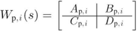
In this work, the Matlab Robust Control Toolbox™ was used to compute the controllers. Because that toolbox provides a solution only to the continuous-time LPV control synthesis problem, the discrete-time plant model Gi,j(z) is converted to the continuous-time plant model Gi,j(s) at the design stage. However, the desired control system operates in discrete-time, therefore the derived continuous-time control law is converted to a discrete-time control law later, prior to implementation. The augmented continuous-time model for controller design is depicted in Fig. 1, where:
Figure 1.

Augmented model for controller design.
| (6) |
r and e are, respectively, the reference and error signals, u is the control action, and Wu,i and Wp,i(s) are the design weights. As shown in Fig. 1, two parameters have been included in each augmented model in order to adapt the controller during the closed-loop implementation. The time-varying parameters are and . The first parameter is real-time measurable and depends on the glucose level g(t) measured by the CGM. The second parameter depends on [ipe(t),ipb], which are the estimated current and basal plasma insulin levels, respectively. The estimation is performed through the subcutaneous insulin model proposed in [37], considering its mean population values. In the case of ipe(t), the input to the model is the current injected insulin, and in the case of ipb, the basal insulin dosage. Note that ipb can be obtained off-line, before the simulation.
In order to design both LPV controllers, the performance and actuator weights are defined as follows:
| (7) |
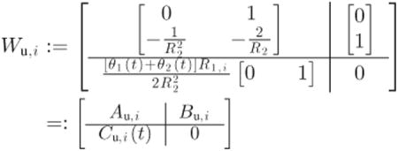 |
(8) |
with T1 = 200, T2 = 105/7, Ai = {8, 7}, α = 3, R1,i = {1/4, 1/8} and R2 = 104/18. Here Cu,i(t) is linear in the time-varying parameters, therefore, as they increase, Wu,i forces a less aggressive control. According to these parameters, both design weights related to 𝒦2,j are defined slightly less conservatively than those related to 𝒦1,j. The weight Wp,i(s) is chosen to be a low-pass filter to induce fast tracking of the safe blood glucose levels. On the other hand, note that in the case of time invariant θ1(t) = θ1(0) = θ10 and θ2(t) = θ2(0) = θ20 ∀t ∈ [0, ∞), then:
| (9) |
is Linear Time Invariant (LTI) and resembles a derivative at low frequencies. Therefore, it helps to penalize fast changes in the insulin delivery. In addition, the model is strictly proper, in order to have the closed-loop system affine in the time-varying parameters.
The parameter θ(t) = [θ1(t), θ2(t)]T is constrained to lie within the rectangular sets 𝒫1 = [0.2, 5] × [0, 8] and 𝒫2 = [0.2, 1] × [0, 8] for 𝒦1,j and 𝒦2,j, respectively. Therefore, both sets 𝒫1 and 𝒫2, which are depicted in Fig. 2, have υ = 4 vertices. The lower and upper bounds of the set 𝒫1 are related to the expected minimum and maximum values of the corresponding variables g(t) and ipe(t), i.e., 20 ≤ g(t) ≤ 550 mg/dl and ipe(t) from 0 to 8 times its basal value. Note that in the case of the set 𝒫2, the maximum value of θ1(t) is unity, i.e., g(t) = 110 mg/dl. As will be shown in Section II-D, that value corresponds to the glucose threshold used by the switching signal algorithm to detect the hyperglycemia condition. An increase in θ1(t) due to a low glucose level and/or in θ2(t) due to a high level of Insulin on Board (IOB) reduces fast and aggressive increases in insulin injection. Because the augmented open-loop model matrices (see Fig. 1 and Eqns. (7) and (8)) depend affinely on the parameter θ(t) = [θ1(t), θ2(t)]T, and that the parameter regions are convex polytopes with a finite number of vertices (see Fig. 2), the optimization problem related to the LPV controller synthesis can be stated in terms of a finite number of Linear Matrix Inequalities (LMIs). Specifically, for each LPV controller, the problem is solved in terms of 2υ + 1 LMIs, i.e., a common Single Quadratic Lyapunov Function (SQLF) for each set of υ = 4 vertices. Note that the vertex controllers can be synthesized off-line.
Figure 2.

Glucose-insulin regions 𝒫1 and 𝒫2.
During the implementation phase, the two LPV controllers for i = 1, 2 can be computed as follows:
| (10) |
| (11) |
where ηℓ(t) ≥ 0 ∀t ∈ [0, ∞) are the polytopic coordinates of the measured parameter θ(t), and θi,ℓ are the vertices of 𝒫i.
One of the problems of the LPV control is known as the “fast poles” problem. By “freezing” any point in the parameter variation set, the resulting LTI model usually presents a small number of poles with a small (i.e., large negative) real part [38], [39]. Fast poles lead to problems from the practical point of view, e.g., integration and/or implementation becomes difficult with these fast dynamics. The approach utilized to deal with these difficulties is LPV pole placement [39]. Through LMI constraints, the objective of the LPV pole placement is to keep the poles of each LTI closed-loop system, resulting from holding the parameter fixed at each point of the parameter variation set, in a prescribed region of the complex plane. Therefore, in order to solve numerical issues in the implementation and/or simulation, for each LPV controller, the (continuous-time) closed-loop poles are constrained to the region , i.e., at least ten times slower than the controller sampling time Ts = 10 min. This pole-placement region forces the closed-loop (frozen) poles not to be faster than 1 × 10⁻³ rd/s in order to obtain a closed-loop response as fast as possible for meal perturbation, but also taking into account that the achievable closed-loop bandwidth is limited since insulin cannot be removed in case of overdelivery [35].
Before implementation, each polytopic LPV controller is converted to a representation which is affine in the time-varying parameters. Finally, a trapezoidal LPV state-space discretization is applied at the implementation stage (see pp. 143-169, [40]).
C. Stability and Performance Analysis
Note that the design was performed by computing a SQLF for each controller. In order to guarantee closed-loop stability and performance under arbitrary switching amongst controllers, a common SQLF is sought for both LPV controllers [41]. The block diagram of the closed-loop is depicted in Fig 3, where:
Figure 3.

Feedback interconnection of plant and controller.
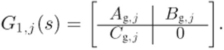
| (12) |
Only G1,j(s) is considered in the analysis, because it represents the “real” transfer-function (G2,j(s) is a fictitious system) and therefore, describes the patient's glucose-insulin dynamics more accurately.
To proceed, the following arguments will be used:
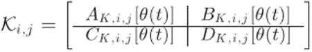
The dependence of the state space matrices AK,i,j [θ(t)], BK,i,j [θ(t)], CK,i,j [θ(t)], and DK,i,j [θ(t)] of both LPV controllers on the parameter θ(t) is affine.
From Eqn. (8), only the output matrix Cu,i of Wu,i is a function of θ(t).
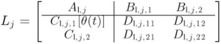
As a consequence, after tedious but straightforward algebra (see Appendix A for the details), the linear fractional interconnection between Lj(s) and the controllers 𝒦i,j as depicted in Fig. 3 produce the following closed-loop state space matrices that are also affine in the parameter θ(t):
| (13) |
| (14) |
| (15) |
| (16) |
Therefore, each affine LPV system can be completely defined by the vertex systems [42], i.e., the images of the υ vertices that make up each parameter set 𝒫i, with i = 1, 2. In this way, the problem consists in seeking, for each Adult #j, a symmetric and positive-definite matrix Xj ∈ ℝn×n, with n the number of closed-loop states, that satisfies the following 2υ + 1 LMIs:
| (17) |
| (18) |
for ℓ = 1, …, υ and i = 1, 2. Here (A, B, C, D)i,j,ℓ is the tuple of the model's closed-loop matrices that result from the feedback interconnection of Lj(s) and 𝒦i,j evaluated at vertex θi,ℓ
By solving one such set of 2υ + 1 LMIs for each patient, the existence of such matrices proved switching stability and performance in all cases. Due to the fact that a more restrictive condition is sought with respect to the design stage, the performance index γ is 30% higher on average for all patients. In any case, this is only a necessary condition, because the final test is performed on the complete adult cohort of the UVA/Padova metabolic simulator in Section III.
D. Switching Signal
As mentioned above, 𝒦2,j is applied only when high and rising glucose values are detected, e.g., after a meal. The block diagram associated with the generation of the switching signal that commands which LPV controller is selected is depicted in Fig. 4. Because of the high measurement noise, some unrealistic hyperglycemic conditions may be detected. Therefore, in order to reduce the number of such false positive detections, the following algorithm, which is similar to the one presented in [33], is defined. The glucose measured by the CGM is filtered by a Noise-spike Filter (NSF), setting to 3 mg/dl/min the maximum allowable glucose Rate of Change (ROC) [43]. Then, gf(t) is filtered by a fourth-order Savitzky-Golay Filter (SGF) [44] to estimate the glucose ROC denoted by ġ̂(t). If gf(t) is higher than 110 mg/dl, and if the last three estimated glucose ROC values are higher than 1.2 mg/dl/min or the last two are higher than 1.4 mg/dl/min, the signal hd(t), which is zero by default, is set to unity by the Hyperglycemia Detector (HD) block. When the latter condition is no longer met, hd(t) is reset to zero. In addition, in order to create a more robust system against the CGM measurement noise, it is considered that hd(t) can be set to unity only if the time period from the last falling edge to the new detection is longer than 30 min. The evolution of the index i that indicates which controller 𝒦i,j is applied, is described by a continuous-time function σ(t) ∈ {1, 2}. The variables ġ̂(t) and hd(t) are inputs to the Switching Signal Generator (SSG) block to define σ(t) as follows. The sampling time after hd(t) is set to unity, σ(t) is set to two when ġ̂(t) ≥ 1 mg/dl/min. Thus, if σ(t) = 2, 𝒦2,j is selected until ġ̂(t) < 1 mg/dl/min, consequently guaranteeing that θ(t) ∈ 𝒫2 while σ(t) = 2.
Figure 4.

Block diagram of the switching signal algorithm. NSF: Noise-spike Filter; SGF: Savitzky-Golay Filter; HD: Hyperglycemia Detector, and SSG: Switching Signal Generator.
III. Results
All in silico adults of the complete UVA/Padova metabolic simulator are considered for simulations, using CGM as the sensor, a generic CSII pump, and with unannounced meals.
The two protocols (see Table I), and the same simulation and analysis conditions used in [28] are employed for controller performance comparison. Note that protocol #1 has a fairly high meal content, whereas protocol #2 has fasting periods. Thus:
The fasting state of each subject is assumed at the start of the simulation.
Open-loop control that infuses the basal insulin is applied during the first 4 hours. After that, the switched LPV controller takes over the insulin delivery until the end of the simulation, with a constant setpoint of 110 mg/dl.
A postprandial period (PP) and night (N) are defined as the 5 hour time interval following the start of a meal, and the period from midnight to 7:00 AM, respectively. In [28], both the Control Variability Grid Analysis (CVGA) plot [45], as well as the average results, are computed based on the results of the third day for protocol #1, and based on the data from the second day for protocol #2. Therefore, to facilitate a direct comparison with the control strategy proposed in [28], in this paper we adopt the same analysis strategy to interpret the results.
Table I.
Protocol # 1 and #2.
| Breakfast 1 | Lunch 1 | Dinner 1 | Breakfast 2 | Lunch 2 | Dinner 2 | Breakfast 3 | Lunch 3 | Dinner 3 | ||||||||||
|---|---|---|---|---|---|---|---|---|---|---|---|---|---|---|---|---|---|---|
|
|
||||||||||||||||||
| Time | gCHO | Time | gCHO | Time | gCHO | Time | gCHO | Time | gCHO | Time | gCHO | Time | gCHO | Time | gCHO | Time | gCHO | |
| #1 | 7 AM | 50 | 2 PM | 60 | 8 PM | 50 | 6 AM | 50 | 1 PM | 70 | 7 PM | 50 | 7 AM | 50 | 1 PM | 65 | 9 PM | 55 |
| #2 | 7 AM | 50 | - | - | 8 PM | 60 | - | - | 12 PM | 55 | 9 PM | 50 | 7 AM | 50 | 2 PM | 55 | 8 PM | 50 |
Here gCHO stands for grams of carbohydrates.
During the implementation phase, the control action u(t) added to the basal insulin ib = Ib,j is delivered by the CSII pump. In order to avoid dangerous scenarios, when σ(t) = 1, gf(t) < 130 mg/dl and ġ̂(t) < −0.3 mg/dl/min, the basal insulin is reduced 25%, i.e., ib = 0.75Ib,j. Based on the small gain theorem [46], the latter does not affect the closed-loop stability.
The average time responses to both protocols are depicted in Fig. 5. The CVGA plots and the average results related to both protocols are presented in Fig. 6 and Table II, respectively. Results for the ℋ∞, approach presented in [28] are also included in Fig. 6 and Table II for comparison. Note that the risk of hyperglycemia is substantially reduced, obtaining a High Blood Glucose Index (HBGI) < 3 with this Proposed Approach (PA). For example, the mean blood glucose is about 15 mg/dl lower, and the percentage of time in the range [70, 180] mg/dl is approximately 25% higher with this approach than with the ℋ∞, one. As a result of this more aggressive tuning, the CVGA plots are shifted to the right but the risk of hypoglycemia is scarcely increased, achieving a minimal Low Blood Glucose Index (LBGI < 1.1). Although a few more subjects are in the D-zone, it is not a problem if that implies an improvement in the general patient population. This is the case because this virtual patient database should be evaluated as a whole population covering different behaviors, and not as individuals. In addition, a more aggressive control action also increases the TDI but again, with no significant increase in the risk of hypoglycemia. Finally, it is worth noting that most of the closed-loop responses are in the upper B-zone. The main reason for that situation is that meals are unannounced, and therefore, blood glucose peaks after meals are difficult to prevent [28], [35], [47].
Figure 5.

Closed-loop responses for all the in silico adults (complete UVA/Padova simulator) to protocol #1 (left) and to protocol #2 (right). The thick lines are the mean values, and the boundaries of the filled areas are the mean ±1 STD values.
Figure 6.

CVGA plots of the closed-loop responses of all in silico subjects (complete UVA/Padova simulator) for the proposed switched-LPV control (stars) and the previous ℋ∞ approach (circles) with respect to protocol #1 (left) and protocol #2 (right). The CVGA categories represent different levels of glucose control, as follows: accurate (A-zone), benign deviation into hypo/hyperglycemia (lower/upper B-zones), benign control (B-zone), overcorrection of hypo/hyperglycemia (upper/lower C-zone), failure to manage hypo/hyperglycemia (lower/upper D-zone), and erroneous control (E-zone). See Table II for zone inclusion percentages.
Table II.
Comparison between the average results for all the adults (complete UVA/Padova simulator) to protocol # 1 and #2 obtained with the Proposed Approach (PA), and with the ℋ∞ strategy proposed in [28].
| Protocol #1 | Protocol #2 | ||||
|---|---|---|---|---|---|
|
|
|||||
| Control Strategy | PA | ℋ∞ | PA | ℋ∞ | |
| Mean BG [mg/dl] | O | 134 | 148 | 134 | 154 |
|
| |||||
| PP | 162 | 176 | 159 | 177 | |
|
| |||||
| N | 101 | 116 | 114 | 135 | |
|
|
|||||
| Max BG [mg/dl] | O | 220 | 226 | 207 | 220 |
|
| |||||
| PP | 223 | 229 | 213 | 224 | |
|
| |||||
| N | 113 | 142 | 153 | 183 | |
|
|
|||||
| Min BG [mg/dl] | O | 90 | 96 | 96 | 108 |
|
| |||||
| PP | 98 | 108 | 103 | 114 | |
|
| |||||
| N | 92 | 100 | 98 | 107 | |
|
|
|||||
| % time in [70 180] mg/dl | O | 83.3 | 75.9 | 86.7 | 75.5 |
|
| |||||
| PP | 67.5 | 54.2 | 71.2 | 54.4 | |
|
| |||||
| N | 99.4 | 99.5 | 99.3 | 91.4 | |
|
|
|||||
| % time > 300 mg/dl | O | 0.0 | 0.1 | 0.0 | 0.0 |
|
| |||||
| PP | 0.1 | 0.3 | 0.0 | 0.1 | |
|
| |||||
| N | 0.0 | 0.0 | 0.0 | 0.0 | |
|
|
|||||
| % time > 180 mg/dl | O | 16.5 | 24.0 | 13.3 | 24.5 |
|
| |||||
| PP | 32.5 | 45.8 | 28.8 | 45.6 | |
|
| |||||
| N | 0.0 | 0.4 | 0.7 | 8.6 | |
|
|
|||||
| % time < 70 mg/dl | O | 0.2 | 0.1 | 0.0 | 0.0 |
|
| |||||
| PP | 0.0 | 0.0 | 0.0 | 0.0 | |
|
| |||||
| N | 0.6 | 0.0 | 0.1 | 0.0 | |
|
|
|||||
| LBGI | 0.3 | 0.1 | 0.1 | 0.0 | |
|
|
|||||
| HBGI | 3.0 | 4.3 | 2.6 | 4.6 | |
|
|
|||||
| TDI [U] | 34.5 | 30.8 | 32.2 | 29.3 | |
The overall (O), and the PP and N time intervals defined previously are analyzed separately.
In order to show how the switching system works, an individual closed-loop response to protocol #1 is presented in Fig. 7. As shown in that figure, when 𝒦2,j is selected (σ(t) = 2), insulin delivery experiences spikes, reducing postprandial glucose levels. The delay between meal ingestion and controller switching is mainly related to the long sensing delays. In addition, it is well-known that high measurement noise appears when CGM is used as the sensor. Despite the noisy CGM signal as depicted in Fig. 8, the controller manages to maintain the blood glucose at a safe level.
Figure 7.

Switching LPV system functioning. Above: The black line is the insulin infusion rate (right axis), the gray line is the blood glucose (left axis), and the asterisks are the CGM measurements. Below: Variation of θ1(t) (gray line) and θ2(t) (black line).
Figure 8.

Closed-loop response for Adult #8, showing noisy CGM signal. The continuous line is the blood glucose concentration, and the asterisks are the glucose measurements via simulated CGM.
The variation of θ(t) = [θ1(t), θ2(t)]T is depicted in Fig. 9. Note that there is a gray narrow stripe around θ1(t) = 1 and 0 ≤ θ2(t) ≤ 1, because θ2(0) = 0, but this subsequently increases until the estimated plasma insulin converges to its steady-state value. As shown in Fig. 9, both parameters evolve within a safe region. This means that when the blood glucose level decreases (θ1(t) increases), the plasma insulin level decreases (θ2(t) decreases), avoiding an overdose of insulin. On the other hand, when the blood glucose level increases (θ1(t) decreases), so does the plasma insulin level (θ2(t) increases), reducing in this way the risk of hyperglycemia. Consequently, dangerous scenarios like low blood glucose values and high plasma insulin levels or vice versa do not occur with this switched LPV approach. Furthermore, the darkest area, which represents the region where both parameters spend the highest percentage of time, is (θ1, θ2) ≃ (1, 1). This means that glucose values are usually around the setpoint (110 mg/dl) without high levels of IOB, despite perturbations like unannounced meals.
Figure 9.
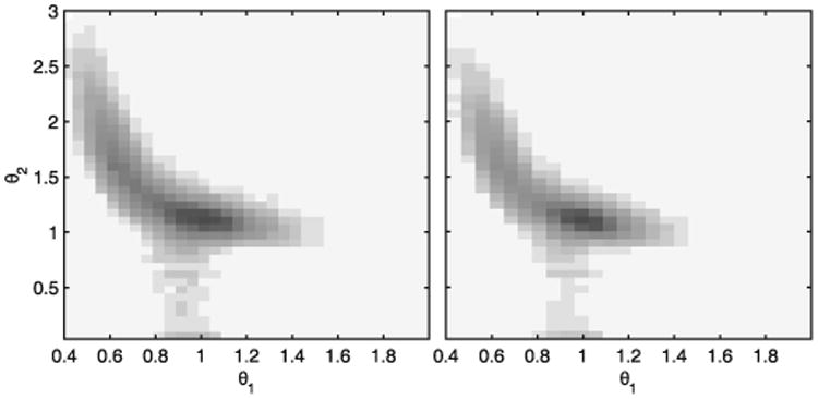
Variation of θ1(t) and θ2(t) parameters for all the in silico adults (complete UVA/Padova simulator) to protocol #1 (left) and to protocol #2 (right).
Although for the design stage both parameters are included in a rectangular region that is larger than the region where the actual time-varying parameters evolve, this conservative choice is necessary in order to have stability and performance guarantees when this is not the case, e.g. due to a large measurement error.
IV. Conclusion
A general switched-LPV controller was designed in order to minimize risks of hyper- and hypoglycemia. This control structure naturally accommodates the time-varying/nonlinear dynamics and intra-patient uncertainty. The controller is based on a model tuned with the patient a priori information in order to cover the inter-patient uncertainty. Finally, a hyperglycemia estimator is used to predict perturbations, e.g., risky postprandial periods. The outcome is an improvement on previous results. The key feature is the possibility of taking into account, at the design stage, important perturbations: unannounced meals and/or patient's physical exercise. Here we have explored the first situation, due to the fact that the UVA/Padova simulator has no physical exercise model. Nevertheless, the same procedure could be applied to the latter situation by either estimating a negative ROC in glucose levels, or through a real-time measurement, e.g., increase in cardiac rhythm.
Acknowledgments
Access to the complete version of the University of Virginia/Padova metabolic simulator was provided by an agreement with Prof. C. Cobelli (University of Padova) and Prof. B. P. Kovatchev (University of Virginia) for research purposes.
P. Colmegna and R. S. Sánchez-Peña were supported by Nuria (Argentina) and Cellex (Spain) Foundations. R. Gondhalekar, E. Dassau and F. J. Doyle III were supported by the following Grants: NIH DP3DK094331 and R01DK085628.
Biographies

Patricio Colmegna received the B.S. degree in automation and control engineering from the National University of Quilmes (UNQ), in 2010, and the doctoral degree in engineering from the Buenos Aires Institute of Technology (ITBA), in 2014. In 2011, he was awarded the National Academy of Engineering Award to the highest grade in engineering. Patricio is currently a postdoctoral researcher at CONICET, and he is also working as a teaching assistant at control systems courses at UNQ. His research interests include modeling, identification and robust control for diverse problems, such as type 1 diabetes mellitus, synchronization between different cerebral structures and mechatronics processes.

Ricardo S. Sánchez-Peña (StM'86-M'88-SM'00) received the Electronic Engineer degree from the University of Buenos Aires (UBA, 1978), and the M.Sc. and Ph.D. from the California Institute of Technology (1986, 1988), both in Electrical Engineering. In Argentina he worked in CITEFA, CNEA and the space agencies CNIE and CONAE. He collaborated with NASA in aeronautical and satellite projects and with the German (DLR) and Brazilian (CTA/INPE) space agencies. He was Full Professor at UBA (1989-2004), ICREA Senior Researcher at the Universitat Politècnica de Catalunya (2005-2009, Barcelona) and visiting Prof./Researcher at several Universities in the USA and the EU. He has consulted for ZonaTech (USA), STI and VENG (Argentina) in aerospace applications and with Alstom-Ecotecnia (Spain) in wind turbines applications. He is recipient of the Premio Consagración in Engineering by the National Academy of Exact, Physical and Natural Sciences (ANCEFN, Argentina) and the Group Achievement Award fom NASA as a Review Board member for the Aquarius/SAC-D satellite. Since 2009 he is Director of the PhD Department in Engineering at the Buenos Aires Institute of Technology (ITBA) and a CONICET Principal Investigator. He has applied Identification and Control techniques to acoustical, mechanical and aero & astronautical engineering and also to type 1 diabetes.

Ravi Gondhalekar (M'10-SM'13) is a Project Scientist at the University of California Santa Barbara (UCSB), USA. His research interests include model predictive control, constrained control and optimization. At UCSB he is applying constrained model predictive control techniques to an artificial pancreas that performs automated delivery of insulin to people with type 1 diabetes. Ravi received a PhD degree in informatics in 2008 from the Tokyo Institute of Technology, Japan, and MEng and BA degrees in engineering in 2002 from the University of Cambridge, UK. From 2008 to 2012 Ravi was an Assistant Professor at Osaka University, Japan. Prior to that he held short-term positions at the Massachusetts Institute of Technology, USA, the University of Cambridge, UK, Princeton University, USA, Pi Technology, UK, the Rutherford Appleton Laboratory, UK, and the United Kingdom Atomic Energy Authority, UK.

Eyal Dassau (M'08-SM'12) received the B.Sc., M.Sc., and Ph.D. degrees in chemical engineering, in 1999, 2002, and 2006, respectively, all from Technion Israel Institute of Technology. He is currently a researcher at the John A. Paulson School of Engineering & Applied Sciences (SEAS), Harvard University, Cambridge, USA. His current research interests include modeling, design and control of an artificial pancreas for type 1 diabetes mellitus. Process and product design with emphasis on medical and biomedical applications. Dr. Dassau is a Senior Member of the American Institute of Chemical Engineering and a member of the American Diabetes Association.

Frank J. Doyle III (M'02-SM'04-F'08) received the B.S.E. degree from Princeton University, Princeton, NJ, in 1985, the C.P.G.S. degree from the University of Cambridge, Cambridge, U.K., in 1986, and the Ph.D. degree from the California Institute of Technology, Pasadena, CA, in 1991, all in chemical engineering.
He is Dean of the John A. Paulson School of Engineering and Applied Sciences (SEAS), Harvard University, Cambridge, USA. His research interests include systems biology, network science, modeling and analysis of circadian rhythms, drug delivery for diabetes, model-based control, and control of particulate processes.
Dr. Doyle is a Fellow of a number of societies including the International Federation of Automatic Control, the American Institute of Medical and Biological Engineering, and the American Association for the Advancement of Science. In 2005, he was awarded the Computing in Chemical Engineering Award from the American Institute of Chemical Engineers for his innovative research in systems biology.
Appendix A: Interconnection Between Lj(s) and 𝒦i,j
Consider that the performance and actuator weights are given by
 |
(19) |
 |
(20) |
and the state-space realization of G1,j(s) has the following form:
 |
(21) |
Then, the augmented open-loop plant Lj(s) can be written as:
 |
(22) |
where
| (23) |
| (24) |
| (25) |
| (26) |
Hence, the linear fractional interconnection between Lj(s) and the corresponding LPV controller
 |
(27) |
yields the closed-loop matrices (13)-(16), which are affine in θ(t).
Contributor Information
P. Colmegna, CONICET, Argentina, and with Departamento de Ciencia y Tecnología, Universidad Nacional de Quilmes, Buenos Aires, Argentina
R. S. Sánchez-Peña, CONICET, Argentina, and with Centro de Sistemas y Control, Instituto Tecnológico de Buenos Aires (ITBA), C1106ACD, Argentina.
R. Gondhalekar, Department of Chemical Engineering, University of California, Santa Barbara, CA, USA.
E. Dassau, John A. Paulson School of Engineering & Applied Sciences (SEAS), Harvard University, Cambridge, USA.
F. J. Doyle, III, John A. Paulson School of Engineering & Applied Sciences (SEAS), Harvard University, Cambridge, USA.
References
- 1.Centers for Disease Control and Prevention. Atlanta, GA: US Department of Health and Human Services, Tech. Rep; 2014. National diabetes statistics report: Estimates of diabetes and its burden in the United States, 2014. [Online]. Available: http://www.cdc.gov/diabetes/data/statistics/2014statisticsreport.html. [Google Scholar]
- 2.Clemens AH, Chang PH, Myers RW. The development of Biostator, a glucose controlled insulin infusion system (GCIIS) Horm Metab Res. 1977;7:23–33. [PubMed] [Google Scholar]
- 3.Hovorka R. Continuous glucose monitoring and closed-loop systems. Diabet Med. 2006;23(1):1–12. doi: 10.1111/j.1464-5491.2005.01672.x. [DOI] [PubMed] [Google Scholar]
- 4.Cobelli C, Dalla Man C, Sparacino G, Magni L, De Nicolao G, Kovatchev BP. Diabetes: Models, signals and control. IEEE Rev Biomed Eng. 2009;2:54–96. doi: 10.1109/RBME.2009.2036073. [DOI] [PMC free article] [PubMed] [Google Scholar]
- 5.Harvey RA, Wang Y, Grosman B, Percival MW, Bevier W, Finan DA, Zisser HC, Seborg DE, Jovanovič L, Doyle FJ, III, Dassau E. Quest for the artificial pancreas: Combining technology with treatment. IEEE Eng Med Biol Mag. 2010;29(2):53–62. doi: 10.1109/MEMB.2009.935711. [DOI] [PMC free article] [PubMed] [Google Scholar]
- 6.Cobelli C, Renard E, Kovatchev BP. Artificial pancreas: Past, present, future. Diabetes. 2011;60(11):2672–2682. doi: 10.2337/db11-0654. [DOI] [PMC free article] [PubMed] [Google Scholar]
- 7.Zisser HC. Clinical hurdles and possible solutions in the implementation of closed-loop control in type 1 diabetes mellitus. J Diabetes Sci Technol. 2011;5(5):1283–1286. doi: 10.1177/193229681100500537. [DOI] [PMC free article] [PubMed] [Google Scholar]
- 8.Phillip M, Battelino T, Atlas E, Kordonouri O, Bratina N, Miller S, Biester T, Stefanija MA, Muller I, Nimri R, Danne T. Nocturnal glucose control with an artificial pancreas at a diabetes camp. N Engl J Med. 2013;368(9):824–833. doi: 10.1056/NEJMoa1206881. [DOI] [PubMed] [Google Scholar]
- 9.Doyle FJ, III, Huyett LM, Lee JB, Zisser HC, Dassau E. Closed loop artificial pancreas systems: Engineering the algorithms. Diabetes Care. 2014;37(5):1191–1197. doi: 10.2337/dc13-2108. [DOI] [PMC free article] [PubMed] [Google Scholar]
- 10.Russell SJ, El-Khatib F, Sinha M, Magyar KL, McKeon K, Goergen LG, Balliro C, Hillard MA, Nathan DM, Damiano ER. Outpatient glycemic control with a bionic pancreas in type 1 diabetes. N Engl J Med. 2014;371(4):313–325. doi: 10.1056/NEJMoa1314474. [DOI] [PMC free article] [PubMed] [Google Scholar]
- 11.Kovatchev BP, Renard E, Cobelli C, Zisser HC, Keith-Hynes P, Anderson SM, Brown S, Chernavvsky DR, Breton MD, Mize LB, Farret A, Place J, Bruttomesso D, Del Favero S, Boscari F, Galasso S, Avogaro A, Magni L, Di Palma F, Toffanin C, Messori M, Dassau E, Doyle FJ., III Safety of outpatient closed-loop control: First randomized crossover trials of a wearable artificial pancreas. Diabetes Care. 2014;37(7):1789–1796. doi: 10.2337/dc13-2076. [DOI] [PMC free article] [PubMed] [Google Scholar]
- 12.Hovorka R, Elleri D, Thabit H, Allen JM, Leelarathna L, El-Khairi R, Kumareswaran K, Caldwell K, Calhoun P, Kollman C, Murphy HR, Acerini CL, Wilinska ME, Nodale M, Dunger DB. Overnight closed-loop insulin delivery in young people with type 1 diabetes: A free-living, randomized clinical trial. Diabetes Care. 2014;37(5):1204–1211. doi: 10.2337/dc13-2644. [DOI] [PMC free article] [PubMed] [Google Scholar]
- 13.Parker RS, Doyle FJ, III, Peppas NA. A model-based algorithm for blood glucose control in type I diabetic patients. IEEE Trans Biomed Eng. 1999;46(2):148–157. doi: 10.1109/10.740877. [DOI] [PubMed] [Google Scholar]
- 14.Cobelli C, Dalla Man C, Sparacino G, Magni L, De Nicolao G, Kovatchev BP. Multinational study of subcutaneous model-predictive closed-loop control in type 1 diabetes mellitus: Summary of the results. J Diabetes Sci Technol. 2010;4(6):1374–1381. doi: 10.1177/193229681000400611. [DOI] [PMC free article] [PubMed] [Google Scholar]
- 15.Breton M, Farret A, Bruttomesso D, Anderson S, Magni L, Patek S, Dalla Man C, Place J, Demartini S, Del Favero S, Toffanin C, Hughes-Karvetski C, Dassau E, Zisser HC, Doyle FJ, III, De Nicolao G, Avogaro A, Cobelli C, Renard E, Kovatchev BP. Fully integrated artificial pancreas in type 1 diabetes: Modular closed-loop glucose control maintains near normoglycemia. Diabetes. 2012;61(9):2230–2237. doi: 10.2337/db11-1445. [DOI] [PMC free article] [PubMed] [Google Scholar]
- 16.Turksoy K, Bayrak ES, Quinn L, Littlejohn E, Cinar A. Multivariable adaptive closed-loop control of an artificial pancreas without meal and activity announcement. Diabetes Technol Ther. 2013;15(5):386–400. doi: 10.1089/dia.2012.0283. [DOI] [PMC free article] [PubMed] [Google Scholar]
- 17.Gondhalekar R, Dassau E, Zisser HC, Doyle FJ., III Periodic-zone model predictive control for diurnal closed-loop operation of an artificial pancreas. J Diabetes Sci Technol. 2013;7(6):1446–1460. doi: 10.1177/193229681300700605. [DOI] [PMC free article] [PubMed] [Google Scholar]
- 18.Cameron F, Niemever G, Wilson D, Bequette BW, Benassi K, Clinton P, Buckingham BA. Inpatient trial of an artificial pancreas based on multiple model probabilistic predictive control with repeated large unannounced meals. Diabetes Technol Ther. 2014;16(11):728–734. doi: 10.1089/dia.2014.0093. [DOI] [PMC free article] [PubMed] [Google Scholar]
- 19.Marchetti G, Barolo M, Jovanovič L, Zisser HC, Seborg DE. An improved PID switching control strategy for type 1 diabetes. IEEE Trans Biomed Eng. 2008;55(3):857–865. doi: 10.1109/TBME.2008.915665. [DOI] [PubMed] [Google Scholar]
- 20.Sherr JL, Cengiz E, Palerm CC, Clark B, Kurtz N, Roy A, Carria L, Cantwell M, Tamborlane WV, Weinzimer SA. Reduced hypoglycemia and increased time in target using closed-loop insulin delivery during nights with or without antecedent afternoon exercise in type 1 diabetes. Diabetes Care. 2013;36(10):2909–2914. doi: 10.2337/dc13-0010. [DOI] [PMC free article] [PubMed] [Google Scholar]
- 21.Mauseth R, Hirsch IB, Bollyky J, Kircher R, Matheson D, Sanda S, Greenbaum C. Use of a “fuzzy logic” controller in a closed-loop artificial pancreas. Diabetes Technol Ther. 2013;15(8):628–633. doi: 10.1089/dia.2013.0036. [DOI] [PubMed] [Google Scholar]
- 22.Nimri R, Muller I, Atlas E, Miller S, Fogel A, Bratina N, Kordonouri O, Battelino T, Danne T, Phillip M. MD-logic overnight control for 6 weeks of home use in patients with type 1 diabetes: Randomized crossover trial. Diabetes Care. 2014;37(11):3025–3032. doi: 10.2337/dc14-0835. [DOI] [PubMed] [Google Scholar]
- 23.Ruiz-Velázquez E, Femat R, Campos-Delgado D. Blood glucose control for type I diabetes mellitus: A robust tracking ℋ∞ problem. Control Eng Pract. 2004;12(9):1179–1195. [Google Scholar]
- 24.Femat R, Ruiz-Velazquez E, Quiroz G. Weighting restriction for intravenous insulin delivery on T1DM patient via ℋ∞ control. IEEE Trans Autom Sci Eng. 2009;6(2):239–247. [Google Scholar]
- 25.Kovács L, Benyó B, Bokor J, Benyó Z. Induced ℒ2-norm minimization of glucose-insulin system for type I diabetic patients. Comput Meth Prog Bio. 2011;102(2):105–118. doi: 10.1016/j.cmpb.2010.06.019. [DOI] [PubMed] [Google Scholar]
- 26.Parker RS, Doyle FJ, III, Ward JH, Peppas NA. Robust ℋ∞ glucose control in diabetes using a physiological model. AIChE Journal. 2000;46(12):2537–2549. [Google Scholar]
- 27.Colmegna P, Sánchez-Peña RS. Analysis of three T1DM simulation models for evaluating robust closed-loop controllers. Comput Meth Prog Bio. 2014;113(1):371–382. doi: 10.1016/j.cmpb.2013.09.020. [DOI] [PubMed] [Google Scholar]
- 28.Colmegna P, Sánchez-Peña RS, Gondhalekar R, Dassau E, Doyle FJ., III Reducing risks in type 1 diabetes using ℋ∞ control. IEEE Trans Biomed Eng. 2014;61(12):2939–2947. doi: 10.1109/TBME.2014.2336772. [DOI] [PubMed] [Google Scholar]
- 29.Colmegna P, Sánchez-Peña RS. Proc 19th IFAC World Congress. Cape Town, South Africa: 2014. Linear parameter-varying control to minimize risks in type 1 diabetes; pp. 9253–9257. [Google Scholar]
- 30.Szalay P, Eigner G, Kovács LA. Proc 19th IFAC World Congress. Cape Town, South Africa: 2014. Linear matrix inequality-based robust controller design for type-1 diabetes model; pp. 9247–9252. [Google Scholar]
- 31.Gondhalekar R, Dassau E, Doyle FJ., III . AACC American Control Conference. Portland, OR, USA: 2014. MPC design for rapid pump-attenuation and expedited hyperglycemia response to treat T1DM with an artificial pancreas; pp. 4224–4230. [DOI] [PMC free article] [PubMed] [Google Scholar]
- 32.Dassau E, Bequette BW, Buckingham BA, Doyle FJ., III Detection of a meal using continuous glucose monitoring: Implications for an artificial β-cell. Diabetes Care. 2008;31(2):295–300. doi: 10.2337/dc07-1293. [DOI] [PubMed] [Google Scholar]
- 33.Harvey RA, Dassau E, Zisser HC, Seborg DE, Doyle FJ., III Design of the glucose rate increase detector: A meal detection module for the health monitoring system. J Diabetes Sci Technol. 2014;8(2):307–320. doi: 10.1177/1932296814523881. [DOI] [PMC free article] [PubMed] [Google Scholar]
- 34.Kovatchev BP, Breton M, Dalla Man C, Cobelli C. In Silico preclinical trials: A proof of concept in closed-loop control of type 1 diabetes. J Diabetes Sci Technol. 2009;3(1):44–55. doi: 10.1177/193229680900300106. [DOI] [PMC free article] [PubMed] [Google Scholar]
- 35.van Heusden K, Dassau E, Zisser HC, Seborg DE, Doyle FJ., III Control-relevant models for glucose control using a priori patient characteristics. IEEE Trans Biomed Eng. 2012;59(7):1839–1849. doi: 10.1109/TBME.2011.2176939. [DOI] [PubMed] [Google Scholar]
- 36.Walsh J, Roberts R. Pumping Insulin. 4th. Torrey Pines Press; San Diego, CA: 2006. [Google Scholar]
- 37.Dalla Man C, Raimondo DM, Rizza RA, Cobelli C. GIM, simulation software of meal glucose-insulin model. J Diabetes Sci Technol. 2007;1(3):323–330. doi: 10.1177/193229680700100303. [DOI] [PMC free article] [PubMed] [Google Scholar]
- 38.Ghersin AS, Sánchez-Peña RS. LPV control of a 6 DOF vehicle. IEEE Trans Control Syst Technol. 2002;10(6):883–887. [Google Scholar]
- 39.Ghersin AS, Sánchez-Peña RS. European Control Conference (Invited paper) Porto, Portugal: 2001. Transient shaping of LPV systems; pp. 3080–3085. [Google Scholar]
- 40.Tóth R. Modeling and Identification of Linear Parameter-Varying Systems. Vol. 403 Berlin Heidelberg: Springer-Verlag; 2010. ser. Lecture Notes in Control and Information Sciences. [Google Scholar]
- 41.Liberzon D. Switching in Systems and Control. Boston, MA: Birkhäuser; 2003. [Google Scholar]
- 42.Becker GS, Packard A. Robust performance of LPV systems using parametrically-dependent linear feedback. Syst Control Lett. 1994;23:205–215. [Google Scholar]
- 43.DeJournett L. Essential elements of the native glucoregulatory system, which, if appreciated, may help improve the function of glucose controllers in the intensive care unit setting. J Diabetes Sci Technol. 2010;4(1):190–198. doi: 10.1177/193229681000400124. [DOI] [PMC free article] [PubMed] [Google Scholar]
- 44.Savitzky A, Golay MJ. Smoothing and differentiation of data by simplified least squares procedures. Anal Chem. 1964;36(8):1627–1639. [Google Scholar]
- 45.Magni L, Raimondo DM, Dalla Man C, Breton M, Patek S, De Nicolao G, Cobelli C, Kovatchev BP. Evaluating the efficacy of closed-loop glucose regulation via control-variability grid analysis. J Diabetes Sci Technol. 2008;2(4):630–635. doi: 10.1177/193229680800200414. [DOI] [PMC free article] [PubMed] [Google Scholar]
- 46.Green M, Limebeer DJ. Linear Robust Control. Englewood Cliffs, NJ: Prentice-Hall; 1995. [Google Scholar]
- 47.Dassau E, Zisser H, Harvey R, Percival M, Grosman B, Bevier W, Atlas E, Miller S, Nimri R, Jovanovič L, Doyle FJ., III Clinical evaluation of a personalized artificial pancreas. Diabetes Care. 2013;36(4):801–809. doi: 10.2337/dc12-0948. [DOI] [PMC free article] [PubMed] [Google Scholar]