

Abstract
Mixture models capture heterogeneity in data by decomposing the population into latent subgroups, each of which is governed by its own subgroup-specific set of parameters. Despite the flexibility and widespread use of these models, most applications have focused solely on making inferences for whole or sub-populations, rather than individual cases. The current article presents a general framework for computing marginal and conditional predicted values for individuals using mixture model results. These predicted values can be used to characterize covariate effects, examine the fit of the model for specific individuals, or forecast future observations from previous ones. Two empirical examples are provided to demonstrate the usefulness of individual predicted values in applications of mixture models. The first example examines the relative timing of initiation of substance use using a multiple event process survival mixture model whereas the second example evaluates changes in depressive symptoms over adolescence using a growth mixture model.
Keywords: mixture models, individual prediction, growth mixture models, person-centered analysis
Recent years have seen a rapid increase in the use of mixture models within the behavioral, health, and social sciences. Examples include latent class analysis (LCA; Lazarsfeld and Henry, 1968), latent profile analysis (LPA; Gibson, 1959), growth mixture models (GMM; Muthén and Shedden, 1999; Nagin, 1999), and the recently introduced multiple event process survival mixture model (MEPSUM; Dean, Bauer, and Shanahan, 2014). An attractive feature of all of these models is that they decompose the population into a small number of groups, referred to as latent classes, that capture heterogeneity in the processes under study (McLachlan and Peel, 2000).
Applications of mixture models can be distinguished by whether the latent classes are thought to represent natural groups or are simply used as a convenient device with which to model individual differences (Titterington, Smith, and Makov, 1985). In direct applications the goal is to identify the number of truly distinct groups in the population and to characterize these groups relative to one another and in relation to potentially relevant antecedents and consequences (e.g., Wiesner and Windle, 2004; deRoon-Cassini, Mancini, Rusch, and Bonanno, 2010). By contrast, the goal of indirect applications is to estimate as many latent classes as necessary to adequately represent the range of individual differences, without concern for the existence or recovery of natural groups. The latent classes are then interpreted to reflect local conditions (Nagin, 2005; Bauer and Shanahan, 2007) or reaggregated to glean insights about the population as a whole (e.g., Kelava, Nagengast, and Brandt, 2014; Pek, Chalmers, Kok, and Losardo, 2015; Gottfredson, Bauer, Baldwin, and Okiishi, 2014). Thus, depending on the nature of the application, inferences may be drawn with respect to the characteristics of the latent classes, the total population, or both.
It is far less common in a mixture analysis for predictions to be made at the level of the individual. This circumstance is at odds with the frequent description of mixture models as being “person oriented” or “person centered” (Bergman and Magnusson, 1997; Muthén and Muthén, 2000; Laursen and Hoff, 2006). Ironically, it is more routine to compute, plot, and potentially make inferences about the predicted values of individuals when fitting continuous latent variable models (e.g., random effects growth models, factor analysis models, item response theory models) despite the fact that these models are generally not regarded as being person centered. Drawing on this parallel literature, we seek to show that similar individual predictions may be made when using mixture models, enhancing both the interpretation and usefulness of the results.
Overall, our goal is thus to demonstrate how the information provided by a mixture model, whether in a direct or indirect application, can be used to make predictions about individuals. Importantly, although there have been a few examples of the use of predicted values in the growth mixture modeling context (Sterba and Bauer, 2014; Nagin and Tremblay, 2005), we believe that this paper provides the first general treatment of individual prediction in mixture models up to this point. Importantly, because mixture models may accommodate virtually any parametric distribution of variables within class, we have sought to present individual prediction in a way that is generalizable to any distributional specification. Drawing on a distinction often made for continuous latent variable models (e.g., Skondal and Rabe-Hesketh, 2009), we explore the computation and use of marginal predicted values, which average over the latent variables, and conditional predicted values, which take into account an individuals’ predicted latent variable scores. We note and demonstrate that different predicted values are suited for different purposes. Additionally, we discuss several different ways of approximating uncertainty around predicted values using parametric bootstrapping (Efron and Tibshirani, 1993). Overall, this emphasis on individual prediction brings the application of mixture models into greater concordance with the goals of a person-centered analytic approach (Bergman and Magnusson, 1997; Bauer and Shanahan, 2007; Sterba and Bauer, 2010).
Mixture Model Formulation
Here we provide a general formulation of the finite mixture model. Defining some initial notation, let i index the individual (where i = 1, 2, …, N) and let k index latent class (where k = 1, 2, …, K). Let us also define a set of K indicator variables, designated cik, that have a value of one when case i is a member of class k and a value of zero otherwise. The values of these indicator variables are unobserved, and the vector ci of the indicator variables has a multinomial distribution. For a given individual, the values of the endogenous variables (e.g., items, indicators, repeated measures) are contained in the p × 1 vector yi, the values of the exogenous variables (e.g., predictors, covariates) are contained in the q × 1 vector xi, and the values of any continuous latent factors that may be present within the model are contained in the r × 1 vector ηi.
The joint distribution of the (observed and latent) random variables given the fixed and known covariates can be factored as follows
| (1) |
where, following Muthén and Shedden (1999), [z] indicates a probability density or mass function for the random variable vector z. Parameter vectors defining the distributions have been suppressed to keep the notation compact (e.g., [ηi|xi, ci] is often specified as a normal distribution for which the parameter vector would consist of conditional factor means, variances, and covariances). Averaging over the latent variables we obtain the marginal distribution for the observed variables:1
| (2) |
Equation (2) expresses [yi|xi] as a finite mixture of k component densities [yi|xi,cik = 1], integrated over ηi and weighted by the mixing probabilities P(cik = 1|xi). For some specifications the integration can completed in closed form (e.g., when the endogenous variables are continuous and both [yi|xi, ηi, ci] and [ηi|xi, ci] are normal), whereas for other specifications numerical approximation methods are required (e.g., when [yi|xi, ηi, ci] is a multivariate Bernoulli distribution for binary endogenous variables and [ηi|xi, ci] is normal).
The mixing probabilities (which sum to one within person) depend on the covariates through a multinomial regression specification, given as
| (3) |
where α0k is an intercept for class k and γk is a q × 1 vector of coefficients conveying the influence of the covariates on the class probabilities. Constraints must be imposed on the values of the parameters in Equation (3) to identify the model; the most common options are to constrain α0k and γk to zero within a reference class, or to estimate an intercept-free model in which all values of α0k are set to zero (see Huang and Bandeen-Roche, 2004 for a review).
In fitting a mixture model, the primary goal is to estimate and make inferences regarding the model parameters or functions of these parameters. These parameters consist of two types, those that define the within-class distributions of the endogenous observed variables and latent factors and those that capture between-class prediction within the multinomial regression. For instance, in a GMM application, one might estimate parameters that define the class-specific growth trajectories of the repeated measures as well as parameters that capture the effects of predictors on class membership. Typically, these parameters are estimated via maximum likelihood; however, Bayesian methods of estimation are sometimes also implemented (Depaoli, 2013; Tueller and Lubke, 2010).
Individual Inference in Mixture Models
Pursuant to the goals of person-centered analysis, it can be particularly interesting to plot the model-predicted values of the endogenous variables for different individuals (either real or hypothetical). Here, we shall define and distinguish between marginal and conditional predicted values. Both have a number of different but complementary uses; each will be explored in turn.
Marginal Prediction
Marginal predicted values summarize what one can predict for the observed endogenous variables based solely upon knowledge of the values of the observed exogenous variables. Since both latent class membership and the values of the latent factors are unknown, marginal predicted values average over these latent variables to arrive at an overall prediction for the endogenous variables. That is, the individual values of the latent variables do not inform the prediction.
Given the marginal mixture distribution in Equation (2), the expected value of yi given xi may be computed as
| (4) |
where E(yi|xi, cik = 1) is the expected value of the within-class marginal distribution [yi|xi, cik = 1]. Designating the sample estimate for P(cik = 1|xi) as and the sample esitmate for E(yi|xi, cik = 1) as , the marginal predicted value may then be defined as
| (5) |
Equation (5) shows the marginal predicted values to be a simple summation of the within-class marginal predicted values, , weighted by the mixing probabilities given the covariates, .
One can compute marginal predicted values for each individual in a sample, for a subset of individuals, or for specific configurations of values for the exogenous variables that might be of interest (irrespective of whether they are observed within the sample, i.e., hypothetical individuals). Although they may be put to a variety of purposes, perhaps the most likely potential use of marginal predicted values is to summarize the predictive relationships implied by the model. For instance, when reporting multilevel and latent growth curve models, it is common to generate and plot predicted trajectories to show how change over time in the repeated measures depends on the values of the predictors (Curran, Bauer & Willoughby, 2004; Preacher, Curran & Bauer, 2006). In this context, usually the values of one or two exogenous predictors are varied while other exogenous predictors are held constant at their means, permitting the isolation of specific effects.
For instance, in one application of GMM, deRoon-Cassini and colleagues (2010) examine the development of PTSD symptoms following traumatic injury over four time points in the six months after initial hospitalization, finding four groups: low-symptom (59%), recovering (13%), delayed (6%), and chronic (22%). Class membership was regressed on self-efficacy at time 1, anger at time 1, educational level, and whether the traumatic injury was caused by human intention (e.g., an attack). Among other effects, membership to the chronic PTSD symptom class was strongly predicted by human intention, OR = 7.67, 95% CI = (2.87–20.49). The authors, in post-hoc analyses, might be interested in probing this difference by calculating and plotting marginal predicted trajectories for subjects whose injuries were caused by human intention, versus those whose injuries were not, holding all other covariates at their sample averages. Additionally, one could plot marginal predicted trajectories according to multiple covariates (e.g., plotting trajectories according to human intention and self-efficacy); even in the presence of only main effects, it can be very informative to visualize the joint nonlinear effects of multiple predictors. We will demonstrate this strategy shortly.
Conditional Prediction
Marginal predicted values incorporate information about only the exogenous variables when generating predictions, averaging over the unknown latent variables. As we will show, however, there are some instances in which we may wish to augment our predictions by considering the most likely values of the latent variables for each individual, which requires incorporating not only covariates xi but also latent class indicators yi. Such inferences can be made through the computation of conditional predicted values, which are based on the expectation of [yi|xi, ηi, ci] from Equation (1). If the latent variables were observed, this expectation could be computed as
| (6) |
This expression differs in two important ways from Equation (4). First, we no longer average over latent classes according to the mixing probabilities. Instead, the expected value depends only on the class to which the individual actually belongs (as cik will equal one only when an individual is a member of class k and will be zero otherwise). Second, we no longer average over latent factors. Within each component the conditional expected value, E(yi|xi, ηi, cik = 1), is computed as the expectation of [yi|xi, ηi, cik = 1], utilizing knowledge of the specific values of the latent factors. That is, the conditional expected value in Equation (6) incorporates information about the latent factors whereas the marginal expected value within Equation (4) does not.
To compute conditional predicted values for a given individual requires that we obtain predictions of the latent variable values for the person. There are many potential ways to compute latent variable scores, both for latent factors (Tucker, 1971; Grice, 2001; Skrondal and Laake, 2001) and latent classes (Bolck, Croon, and Hagenaars, 2004; Lanza, Tan, and Bray, 2013; Vermunt, 2010). We do not delve into this extensive literature here. As is common, for the present purposes, we shall use empirical Bayes’ predictors for the latent variables, which take into account both the observed values of yi as well as xi. While it may be somewhat counterintuitive to use yi to predict ci and ηi and then use the estimated values of ci and ηi to predict yi, these sorts of predictions (referred to sometimes as “post-dictions,” e.g., Skrondal and Rabe-Hesketh, 2009, p. 674) are quite commonly used in multilevel models and IRT to assess model-based predicted values of yi against observed values; these uses will be explored shortly.
For latent class membership, we shall calculate posterior probabilities of class membership. The posterior probabilities are given by Bayes’ Rule as
| (7) |
When computed using the model estimates in place of the population parameter values, the posterior probabilities constitute emprical Bayes’ predictors and will be denoted .
Prediction of the factor scores is similarly based upon their posterior distribution. The posterior distribution of ηi given yi, xi, and class membership is given by Bayes’ Rule as
| (8) |
Taking the expectation of [ηi | yi, xi, cik = 1] yields the expected values of the factors for person i assuming he or she is a member of class k. Since class membership is unknown, there are K possible expected values for each individual, one for each latent class to which the individual may be a member. As before, in computing the class-specific expected values, the model estimates are substituted for the population parameters, making these emprical Bayes’ predictors of the factor scores. Factor scores computed in this manner are commonly referred to as expected a posteriori scores (EAPs; Bock and Aitkin, 1981). We shall denote the EAPs as .
Using these empirical Bayes’ predictors for the latent variables, the sample analog to Equation (6) for computing conditional predicted values is then
| (9) |
where is the vector of within-class conditional predicted values obtained based on the predicted factor scores, .
Similar to marginal predicted values, one may compute conditional predicted values based upon any configuration of values for xi and yi, whether these are observed within the sample or simply represent a subset of possible configurations of interest. There are also many potential uses of conditional predicted values. First, they may be used to judge the correspondence between the predicted and observed values for a specific individual, taking into account the latent class structure of the model (rather than averaging over classes). In this way the conditional predicted values may be used to judge the “person fit” of the model, a strategy which has been used extensively in IRT studies (Reise, 2000). In this context, the strength of the assocation between the individual’s estimated ability and their observed score is then used as a measure of person-fit, with weak associations indicating potentially aberrant responding (Woods, Oltmanns, and Turkheimer, 2008; Conijn, Emons, de Jong, and Sijtsma, 2015). Similarly, in mixture models, it may be of interest to gauge concordance between predicted and observed values for a random subset of individuals or for selected individuals based on their most likely class. For instance, in the PTSD example discussed earlier (deRoon-Cassini et al., 2010), one could examine whether individuals in some classes more closely follow their predicted trajectories than in other classes, or identify specific individuals, regardless of class, whose trajectories are poorly predicted by the model.
Second, conditional predicted values may be used to visualize the range of individual differences implied by a model. For instance, in growth modeling applications, plotting conditional predicted values for the repreated measures provides a visual depiction of the full range of individual differences in change over time (rather than just those differences that may be ascribed to the exogenous predictors; Raudenbush, 2001). Finally, one may use incomplete information on the endogenous variables when computing the posterior predicted values to generate predictions about the remaining endogenous variables. Dean, Cole, and Bauer (2015) used this strategy in a survival mixture model of substance abuse initiation in adolescence; given substance use data at age 13, they predicted the pattern of substance use initiation throughout adolescence and young adulthood.
In sum, when fitting a mixture model, we can make individual predictions using either marginal or conditional predicted values. Marginal predicted values take into account only the values of the exogenous variables, whereas conditional predicted values also take into account the predicted values of the latent variables for the individual. Marginal predicted values are well suited to visualizing relationships between exogneous and endogneous variables, averaging over the latent variables. Conditional predicted values are well suited for making individual predictions that are informed by the latent variables, and can be used to evaluate person fit, to visualize individual differences, or for forecasting purposes (among other possibilities). Regardless of the type or use of predicted values, however, an important consideration is that they are computed using sample estimates for the model parameters. Thus, prior to illustrating the use of these predicted values we shall consider how best to represent their uncertainty due to sampling error.
Quantifying Uncertainty around Individual Predictions
There are a number of ways to consider uncertainty around the model-implied predicted values given by Equations (5) and (9). One possibility is to alter the prediction intervals developed by Skrondal and Rabe-Hesketh (2009) for random effects models for use with mixture models. Another option is to use parametric bootstrap methods (Efron and Tibshirani, 1993) to generate a number of hypothetical sets of predicted values from the model. This latter approach, which we pursue here, quantifies uncertainty in the individual predicted values by empirically approximating the sampling distribution of the model parameters upon which the predicted values are based. We first discuss the computation of confidence intervals (CIs) for the point estimates of the predicted values and and then consider the computation of prediction intervals (PIs) for the obsevations yi based upon these predicted values.
Confidence Intervals
Let us designate the full vector of model parameters as θ. Under certain assumptions, the maximum likelihood estimates of the model parameters, , are asymptotically normally distributed around the true parameter values θ, as follows:
| (10) |
Here, represents the variance-covarince matrix of the estimates .
The parametric bootstrap strategy, described in detail by Pek, Losardo, and Bauer (2011), consists of making some number B of bootstrap draws (e.g., 5000) from the estimated sampling distribution of the parameter estimates. More specifically, the bootstrap distribution substitutes the maximum likelihood estimates and the estimated covariance matrix of the estimates for their population counterparts, as follows:
| (11) |
Draws are then taken from this distribution to construct confidence intervals for or .
With each draw from the bootstrap distribution, a new set of marginal or conditional predicted values is calculated based upon (where b = 1, 2,…, B). These values, which we shall designate and , respectively, are computed as shown in Equations (5) and (9), with the exception that the bootstrapped parameter estimates are used in the computations (rather than original model estimates, ), including when obtaining latent variable scores for conditional predicted values. Using this procedure we can obtain an empirical distribution of marginal and/or conditional predicted values that reflects the uncertainty of the parameter estimates upon which they are based. It may be particularly informative to construct plots of the bootstrapped values. Specifically, to visualize uncertainty due to sampling error, we may plot either the boostrapped marginal or conditional predicted values or , respectively, around the original (mean) values or .
The set of B bootstrapped values obtained for any given individual may thus be used to quantify and/or visualize sampling error about the individual predicted values. For instance, for any given endogenous variable, the 2.5th and 97.5th percentiles of the empirical distribution of predicted values demarcate a 95% bootstrapped confidence interval. For marginal predicted values, the procedure for generating bootstrapped confidence intervals may be summarized as follows:
Simulate B draws from . Denote each vector of parameters as .
For each set of parameter values, obtain the class-specific expected value for each class. Calculate prior probabilities of class membership for case i using Equation (3), and aggregate across classes using Equation (5) in order to obtain .
Choose the 97.5th and 2.5th values of from the B draws; these demarcate the bounds of a 95% CI.
For conditional predicted values, the procedure is varied to incorporate the latent variable scores:
Simulate B draws from . Denote each vector of parameters as .
For each set of parameter values, calculate subject i’s conditional expected value (or EAP) for each class by taking the expectation of the distribution given by Equation (8); use this value to obtain class-specific conditional expected values . Calculate posterior probabilities of class membership for case i using Equation (7), and aggregate across classes using Equation (9) in order to obtain .
Choose the 97.5th and 2.5th values of from the B draws; these demarcate the bounds of a 95% CI.
Prediction Intervals
The above procedure describes confidence intervals for the predicted values and . These intervals indicate sampling error in the estimated expected value of yi over repeated sampling, either marginalizing over the latent variables (with ) or conditioning on their values (with ). In some instances, however, we may be interested in conveying uncertainty in the potential observed values of yi (or any of its individual elements ) that correspond to these predicted values; that is, given the predictors and perhaps also including knowledge of and . Prediction intervals indicate the range of values of yi that might be observed for a real or hypothetical individual within a specified probability (e.g., 95% of the time; Skrondal and Rabe-Hesketh, 2009; Kutner, Nachtsheim, and Neter, 2004, pp. 56–60).
Whereas a CI for or takes into account variability in the parameter estimates , a PI also must take into account the variance of the random variables in the model, for which the realized values will vary across observations. When computing a marginal prediction interval, the random variables include , , and yi ; whereas when computing a conditional prediction interval the latent variable values are treated as known and the only random variables are contained within yi. The two types of prediction intervals have different uses. For instance, marginal prediction intervals are useful for predicting new observations for new individuals whereas conditional prediction intervals are useful for predicting new observations for individuals for whom some data has already been collected (i.e., individuals in the sample).
In order to make prediction intervals for a new observation of yi, we augment the resampling procedure outlined above by taking draws from the conditional distributions of the random variables. This strategy, borrowed from the multilevel modeling literature (Kovacevic, Huang, and You, 2006; van der Leeden, Meijer, and Busing, 2008, pp. 401–419), involves successively drawing from each distribution as follows. For marginal prediction intervals:
Simulate B draws from . Denote each vector of parameters as .
- For each set of parameter values:
- Draw class membership: Using the bootstrapped parameter values, compute the prior probabilities of class membership using Equation (3); take one random draw of class membership from the multinomial distribution with probabilities .
- Draw : Given membership to class k obtained from step (a), take one random draw from the class-specific marginal distribution of continuous latent variables for subject i’s assigned class, .
- Draw from the predicted distribution of y : Given the class membership assigned in step (a) and the value of obtained from step (b), take one random draw, denoted , from the implied distribution of yi values for the individual, .
Choose the 97.5th and 2.5th values of from the B draws; these demarcate the bounds of a 95% PI around .
For conditional prediction intervals:
Simulate B draws from . Denote each vector of parameters as .
- For each set of parameter values:
- Draw class membership: For each class, compute the posterior probability of class membership using Equation (7); take one random draw of class membership from the multinomial distribution with probabilities .
- Draw : Given membership to class k obtained from step (a), take one random draw from the class-specific posterior distribution of continuous latent variables for subject i’s assigned class, .
- Draw from the predicted distribution of y: Given the class membership assigned in step (a) and the value of obtained from step (b), take one random draw, denoted , from the implied distribution of yi values for the individual, .
Choose the 97.5th and 2.5th values of from the B draws; these demarcate the bounds of a 95% PI around .
Importantly, prediction intervals and confidence intervals are both centered around the same expected values, i.e., or , but will differ in width to afford different inferences, with PIs being wider than CIs to encompass the additional range of variability in potential realized values associated with any given expected value.
In summary, by making use of resampling procedures, we may compute confidence intervals around predicted values of yi to convey the uncertainty of the estimates; further, we may compute prediction intervals by adding another resampling step which accounts for variation in the realized values associated with any given predicted value.
Assumptions of the resampling approach
The parametric bootstrap offers a relatively computationally inexpensive way of obtaining intervals when analytical derivations require approximations or are otherwise intractable, as would often be the case for the models considered here. A fully non-parametric solution, which would involve re-estimation of the model on B re-drawn samples from the raw data, would be considerably more expensive computationally and potentially infeasible (Yung and Bentler, 1996; Davison and Hinkley, 1997, pp. 15–22).
It is important to recognize, however, that the parametric bootstrap approach invokes a number of assumptions that must be met to yield valid coverage rates. Above all, it assumes that the parametric specification of in Equation (10) is correct – i.e., that is a consistent estimator of θ, that is asymptotically normally distributed, and that the sample size is sufficiently large to approach asymptotics. Whether these properties hold will depend on the estimator of θ, with each method of estimation invoking its own set of assumptions. For normal theory maximum likelihood, Satorra (1990) divides these into structural assumptions, such as the inclusion of all relevant variables and correct specification of the relationships between them; and distributional assumptions, including that errors are normally distributed and homogenous across all levels of predictors and outcomes (i.e., homoscedasticity), and observations are independent and indentically distributed. Also included in this latter category is that the distributions of the latent and observed variables are specified correctly (e.g., normal, binomial, Poisson). Within mixture models, both structural and distributional misspecification can compromise class enumeration procedures and lead to inconsistent within-class estimates even when the correct number of classes is selected (Bauer and Curran, 2003; 2004; Hoeksma and Kelderman, 2006; Morin, Maiano, Nagengast, Mars, Morizot, and Janosz, 2011; Van Horn et al., 2012).
The parametric bootstrap also requires that is a consistent estimator of in Equation (11). Under normal-theory ML, is given by the inverse of the expected Fisher information matrix (Eliason, 1993); may be estimated as the second derivative of the log-likelihood evaluated at the MLE (i.e., the observed Fisher information matrix; Efron and Hinkley, 1978). Because there is typically no closed-form analytic solution for when the expectation-maximization (EM; Dempster, Laird, and Rubin, 1977) algorithm is used, is evaluated numerically by most statistical packages using the method of Louis (1982); this is the method used here. The naïve estimate of will be consistent under the same structural and distributional assumptions described by Satorra (1990). Note, however, that there are alternative ways to compute with varying degrees of robustness to model misspecification (Arminger and Schoenberg, 1989; Browne and Arminger, 1995), non-normality (when distributions are specified as normal; Satorra and Bentler, 1994; Yuan and Bentler, 1997), and heteroscedasticity (Huber, 1967; White, 1982).
Thus, if the assumptions of the normal-theory ML estimator are met then parametric bootstrap estimates of variability should also show good asymptotic performance and nominal coverage rates. By implication, considerable attention should be paid to the specification of the model when implementing parametric boostrapping (Efron and Tibshirani, 1993; Preacher and Selig, 2012). Without intending to discount the importance of avoiding specification errors, it is also worth recognizing that research on indirect applications of mixture models have documented good performance for estimates and inferences made by aggregating information over classes, despite the fact that the fitted model is not literally correct in the population (Bauer, Baldasaro and Gottfredson, 2012; Nagin, 2005, p. 48–54; Pek, Losardo, and Bauer, 2011; Sterba and Bauer, 2014). Thus, although additional research is needed on this point, the predicted values and and associated CIs and PIs may be relatively robust to the violation of structural and/or distributional assumptions, provided the model is specified in a way that the estimated parameters are still able to capture the primary features of the data generating process.
We now turn to two empirical demonstrations of the utility of individual predictions in mixture models.
Empirical Example 1: Patterns of Substance Use Initiation
For our first example, we revisit an application of a multivariate survival mixture model to trajectories of substance use initiation in adolescence. The goal of this analysis was to characterize patterns of onset of substance use across multiple categories of licit and illicit drugs (e.g., alcohol, tobacco, marijuana, cocaine). Here we shall build upon this analysis by focusing specifically on predicting the onset of harder drug use based on the time of initiation of alcohol and marijuana use.
Sample and Measures
Data come from the National Survey on Drug Use and Health (NSDUH), and consist of substance use initiation questionnaires taken from respondents on a yearly basis between ages 10 to 30. Subjects (N = 55,772 ; 52% female) were asked whether and at what age they initiated use of the following substances: alcohol, tobacco, marijuana, non-medical use of prescription drugs (NMUP), hallucinogens, cocaine, inhalants, stimulants, or heroin. The sample was ethnically diverse, with 62% of respondents categorized as Caucasian, 13% as African American, 16% Hispanic, and 9% as other. Sex and ethnicity were included in the model as covariates. A more detailed description of the data and sample are available in Dean, Cole, and Bauer (2015).
Model Fitting
The model applied to the data is the multiple event process survival mixture (MEPSUM) model introduced by Dean, Bauer, and Shanahan (2014). Briefly, the MEPSUM model characterizes the relative timing of multiple events. For each of the nine drug classes, a binary indicator variable was created at each age which was scored zero if the event had not yet occurred, one if the event occurred at that specific age, and missing otherwise (i.e., if the event had already occurred or the individual was not observed at that age, indicating censoring). The vector of indicator variables constitutes the endogenous variables for the model, or yi.
The MEPSUM model conforms to Equation (2) with [yi | xi, ηi,cik = 1] defined by assuming that the indicator variables within yi are conditionally independent and Bernoulli distributed. The probability parameters, which in this case correspond to hazard rates, vary across classes and will be designated hik. In the current application, we implemented the logistic link function for the hazards and modeled change in the logit for each substance as a quadratic function of age. Similar to a multivariate growth model, this entailed the definition of a latent intercept, linear change, and quadratic change factor for each substance. Thus, the model was defined as
| (12) |
where νik is the vector of logits corresponding to hik. The factor loading matrix Λ was defined to be equal across classes (hence the absence of a k subscript) and to consist of nine blocks reflecting quadratic change for each susbtance. Specifically, using decade as the metric of time, the block of factor loadings corresponding to any given substance s was specified as
| (13) |
Each block thus defined three factors, for a total of 27 factors across the nine substances. Contrasting with a standard multivariate growth analysis, in the MEPSUM model the variances and covariances of the factors are all set to zero, i.e., Ψk = 0 ; only the factor means αk are estimated (hence the within-class distribution for the continuous latent variables drops out of Equation (2) and the integral resolves). Class-membership was regressed on coding variables representing sex and ethnicity using the multinomial specification given in Equation (3). Finally, for conveying results, the model-implied hazards are cumulated to produce lifetime distribution functions (see Dean, Bauer & Shanahan, 2014, for computational details).
Full details of model fitting and estimates are available in the original report (Dean, Cole, and Bauer, 2015). In brief, fit indices favored a six-class solution, shown in Figure 1. A plurality of subjects fell into the “abstainer” class (35.7%), characterized by a low risk of any substance use over time. Users of soft drugs (alcohol, tobacco, and marijuana) fell into three remaining classes, characterized by late onset of soft drug use (26.7%), early onset of soft drug use (12.1%), and a progressive, steady hazard of initiating soft drug use (8.2%). Users of hard drugs (predominantly cocaine, hallucinogens, and NMUP) fell into the remaining two classes: late hard drug onset (10.9%), and early hard drug onset (6.3%).
Figure 1.
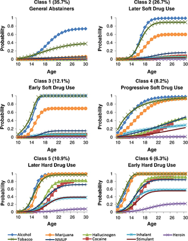
Empirical example 1: Cumulative probability of substance use initiation over time.
Note. Figure originally appears as Figure 4 in Dean, Cole, and Bauer (2015).
Individual Predictions
For this model, we focus on conditional predicted values; however, for completeness we also provide the formula for marginal predicted values. Specifically, for this model the marginal predicted values in Equation (5) correspond to
| (14) |
where may be interpreted as the predicted hazard rate given the covariate scores, averaging over latent classes. Here, is the model-implied marginal hazard rate within class k, calculated by first computing the predicted logit as and then inverting the logistic link function to obtain the predicted probability (expected value) corresponding to each element in .
Similarly, the conditional predicted values in Equation (9) are computed as
| (15) |
and may be interpreted as the predicted hazard for person i given her values for the covariates as well as her posterior predicted class membership. Here, is the predicted hazard conditional on the individual’s latent factor scores and is calculated by computing the predicted logit within class k as and applying the inverse link function. In this case, because the variances of the latent factors are null, the predicted factor scores collapse to the class means, and . Thus, since in this model there is no within-class variation in the factor scores, and the only difference between the marginal predicted values in Equation (14) and the conditional predicted values in Equation (15) is whether the within-class hazards are weighted by the predicted or posterior class probabilities. Weighting by the predicted probabilities averages over classes, whereas weighting by the posterior probabilities conditions on the individual’s class membership.
In the current application we used conditional predicted values to evaluate the likelihood of engaging in hard drug use given early involvement in softer drug use. A number of studies have linked the early use of marijuana (Robins, Darvish, and Murphy, 1970; Kandel, 2002) to later hard drug use. Given growing concerns about the abuse of prescription medications (Boyd, McCabe, Cranford, and Young, 2006; Compton and Volkow, 2006), we centered our examination on NMUP onset and how it may vary depending on the timing of onset of marijuana use, holding alcohol use constant. Conditional predicted values are best suited to evaluating this question because the observed timing of marijuana use can be used to provide information on class membership. We computed conditional predicted values for NMUP for two hypothetical individuals: (a) a Caucasian male subject with alcohol use onset at age 12 and marijuana use onset at age 13; and (b) a Caucasian male subject with alcohol use onset at age 12 and marijuana use onset at age 16. In computing the posterior probabilities of class membership from Equation (7) we coded all of the remaining indicator variables in yi as missing (unobserved). For ease of interpretation, we used the predicted hazards for these individuals to compute lifetime distribution functions.
The predicted lifetime distribution functions are shown as the solid bold lines in Figure 2. To convey the sampling error in these predicted values, we also generated and plotted B = 2500 bootstrapped estimates of the predicted values. The plotted intervals are point-wise confidence intervals as opposed to prediction intervals; thus, they convey uncertainty in the expected survival function. Examination of these functions indicates that for both subjects the lifetime probability of NMUP use increases rapidly over adolescence and then begins to asymptote in the early 20’s. Earlier initiation of marijuana use, however, results in an earlier, more rapid, and more pronounced increase in the likelihood of NMUP use. By age 20, an early-onset marijuana user has a roughly 70% probability of having engaged in NMUP, compared to approximately 40% for the late-onset marijuana user.
Figure 2.
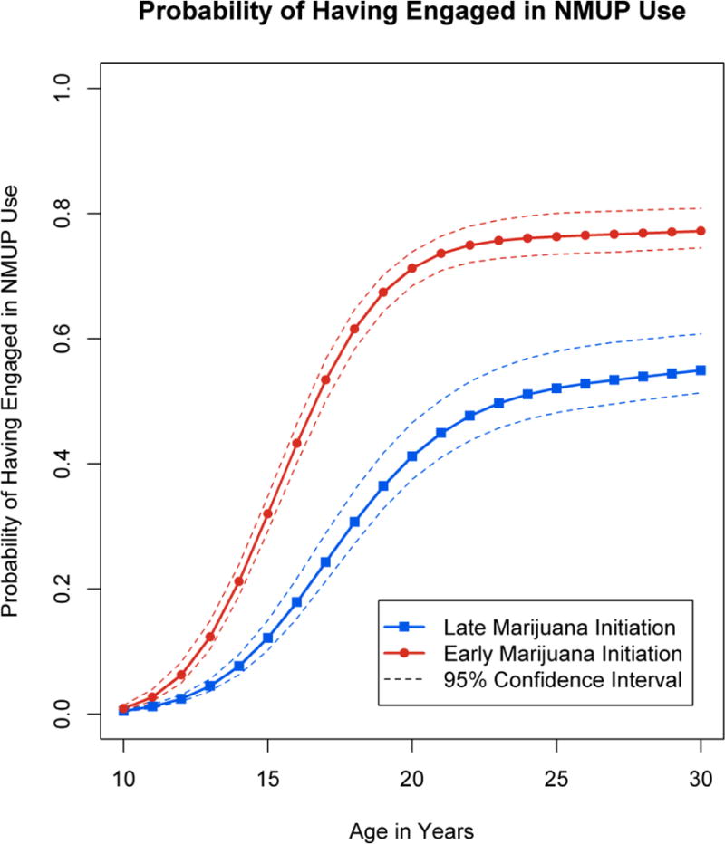
Empirical example 1: Predicted probability of nonmedical prescription drug use for two subjects differing in age of marijuana use initiation.
In sum, this application illustrated how conditional predicted values can be used for forecasting purposes. A subset of the endogenous variables (referencing marijuana and alcohol use) was used to infer posterior probabilities of class membership, which in turn were used to generate conditional predicted values for other endogenous variables at later points in time (and for other substances). In this manner we were able to enhance our understanding of the interdependence of substance use onset times implied by the MEPSUM model, in particular, the relation between early marijuana use and NMUP use.
Empirical Example 2: The Development of Depressive Symptomatology
For our second example, we demonstrate how to plot predicted trajectories from a growth mixture model, with a specific focus on changes in depressive symptoms during the transition from adolescence to adulthood.
Sample and Measures
Data were drawn from the 1997 National Longitudinal Survey of Youth (NLSY97). For the purposes of this demonstration, we included data for individuals who were 14 years old in 1997 from assessments made in 2000, 2002, 2004, 2006, 2008, and 2010 (i.e., during the transition to adulthood), and for whom no more than half of the selected repeated measures were missing (N = 1460). The sample was 51% male, and relatively ethnically diverse, with 27%, 19%, 1%, and 53% of respondents identifying as Black, Hispanic/Latino, mixed race, and neither Black nor Hispanic/Latino, respectively.
The main outcome of interest, depression, was measured as the sum of five 4-point items from the Center for Epidemiological Studies Depression scale (CES-D). Potential values range from 5 to 20, with higher values indicating higher levels of depression. Predictors include race (coded 0 for non-Black/non-Hispanic/Latino, 1 otherwise), gender (coded 1 for males, 0 for females), parent-rated physical health (coded from 1–5, with lower scores representing better overall health) and college attendance (coded as 1 if the subject attended college by age 23, 0 otherwise). The latter predictor was included based on research indicating that clinical patterns among college students may differ from their non-college-attending counterparts (Gfroerer, Greenblatt, and Wright, 1997; Blanco et al., 2008).
Model Fitting
The GMM fit to the data allowed for maximum flexibility in the shape of change over time observed within classes and was initially described in detail by Ram and Grimm (2009). In brief, whereas a typical GMM might constrain growth within each class to follow a linear or lower-order polynomial function, here we estimate the functional form of growth freely within each class via a freed-loading latent basis model (Meredith and Tisak, 1990).
With reference to Equation (2), in the current application we assumed that, conditional on the latent growth factors, the repeated measures are normally distributed within classes; that is [yi | xi, ηi,cik = 1] references a normal distribution with conditional mean vector μik and covariance matrix Σk. These conditional moments are structured according to a latent growth model such that
| (16) |
where J is the number of repeated measures, σjk2 is the residual variance of each repeated measure at time j in class k, and DIAG() is an operator which places the enclosed elements in a diagonal matrix, implying that the repeated measures are conditionally independent.
Each class-specific matrix of factor loadings, Λk, was minimally constrained to define a latent intercept and shape factor, as follows:
| (17) |
Similarly, we assumed the latent growth factors to be normally distributed within classes such that [ηi | xi,cik = 1] references a normal distribution with mean vector αk and variance-covaraince matrix Ψk. Each of the elements of the mean vector αk was freely estimated; however, to decrease model complexity and facilitate model convergence, only the variance of the intercept was estimated and it was constrained to equality across classes; thus
| (18) |
Since both [yi | xi, ηi,cik = 1] and [ηi | xi,cik = 1] are normal, the within-class marginal distribution of the repeated measures [yi | xi,cik = 1] in Equation (2) resolves to a normal probability distribution with an implied mean vector of Λkαk and covariance matrix of . Last, covariate effects on class membership were modeled via the multinomial regression specification given in Equation (3).
As in any application, one could consider alternative model specifications to the one used here. For instance, if the within-class distributions of depression are thought to be skewed, then one might specify [yi|xi,ηi,cik = 1] as a skew-normal distribution (Asparouhov and Muthén, 2016). Likewise, one could consider alternative specifications of the within-class covariance matrix for the latent factors. Without a strong basis for advocating for one specification over another, we sought here to implement the simplest model specification that we believed would adequately capture individual differences in change over time.
Models with successively larger numbers of classes were tested, and a 3-class model was chosen on the basis of the Bayesian Information Criterion (BIC; Schwarz, 1978), which balances fit and parsimony, (BIC = 34343.96, 34334.82, and 34349.38 for models with 2, 3, and 4 classes, respectively). In order to determine whether free estimation of the functional form of growth was necessary, we also examined the fit of a 3-class linear GMM; we found the freed-loading GMM to fit significantly better than the corresponding linear model, χ2(12) = 97.30, p < .001. The residual variance of the indicators σjk2 was also allowed to differ over classes k and time points j; this parameterization showed significantly better fit than a model in which residual variance was constrained to be equal across time, χ2(15) =85.55, p < .001, or across classes, χ2(12) = 786.33, p < .001.
Figure 3 shows the predicted trajectories for these three classes. A plurality of cases (40.2%) falls into Class 1, which is characterized by generally low levels of depressive symptoms which decrease very slightly over time. The other two classes are characterized by either a pattern of symptoms which start out relatively low but increase linearly (Class 2; 23.9%), or high overall levels of symptoms which remain relatively stable and decrease very slightly (Class 3; 35.9%). Of the covariate effects examined, gender and college attendance were the only significant predictors of class membership. Membership to Class 3, which was characterized by high overall levels of depressive symptoms, was positively associated with being female and negatively associated with college attendance. Specifically, women were significantly more likely to be in Class 3 than Class 1, γ = 0.362, z = 2.156, p = .031 or Class 2, γ = 0.869, z = 3.541, p < .001. College non-attendees were significantly more likely to be in Class 3 than Class 1, γ = 1.018, z = 5.661, p < .001, or Class 2, γ = 0. 805, z = 2.970, p = .003. To better understand the results of the model we will now compute predicted values. Marginal predicted values will be used to visualize the effects of the covariates, whereas conditional predicted values will be used to evaluate the person fit of the model.
Figure 3.
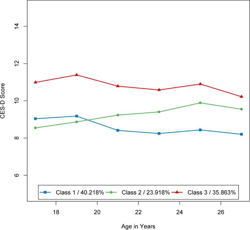
Empirical example 2: Mean trajectories and class membership proportions for each class.
Individual Predictions
The analysis at the whole-sample level suggested that both gender and college attendance are linked to depressive symptoms. To better understand this relationship, we computed marginal predicted values for four hypothetical individuals, varying the values of gender and college attendance, but holding all non-focal covariates at their sample averages. For this model, the marginal predicted values in Equation (5) may be expressed as
| (19) |
Thus, based on the covariate values, we first obtained the predicted probabilities of class membership .. Then, weighting the model-implied estimated class mean trajectories by these probabilities, we obtained the marginal predicted trajectories shown in the top panel of Figure 4. These predicted trajectories help to clarify the nature of the predictor effects, showing how, over this span of development, depressive symptoms are more severe in women, and in those who did not attend college. The shape of change is consistent, generally declining with age with the exception of episodic increases at 19 and 25 years of age. We generated marginal 95% confidence intervals using B=2500 for these trajectories. As shown in the top panel of Figure 4, the set of plausible values overlaps almost completely for male and female participants; however, as shown in the bottom panel, the trajectories diverge somewhat more between college attendees and non-attendees. This is an informative finding, as it contextualizes the results from the covariate logistic regression: though both college attendance and gender had significant effects on membership to a more highly symptomatic class, the overall predicted difference between college attendees and non-attendees in the development of depressive symptoms is more robust than that between male and female participants.
Figure 4.
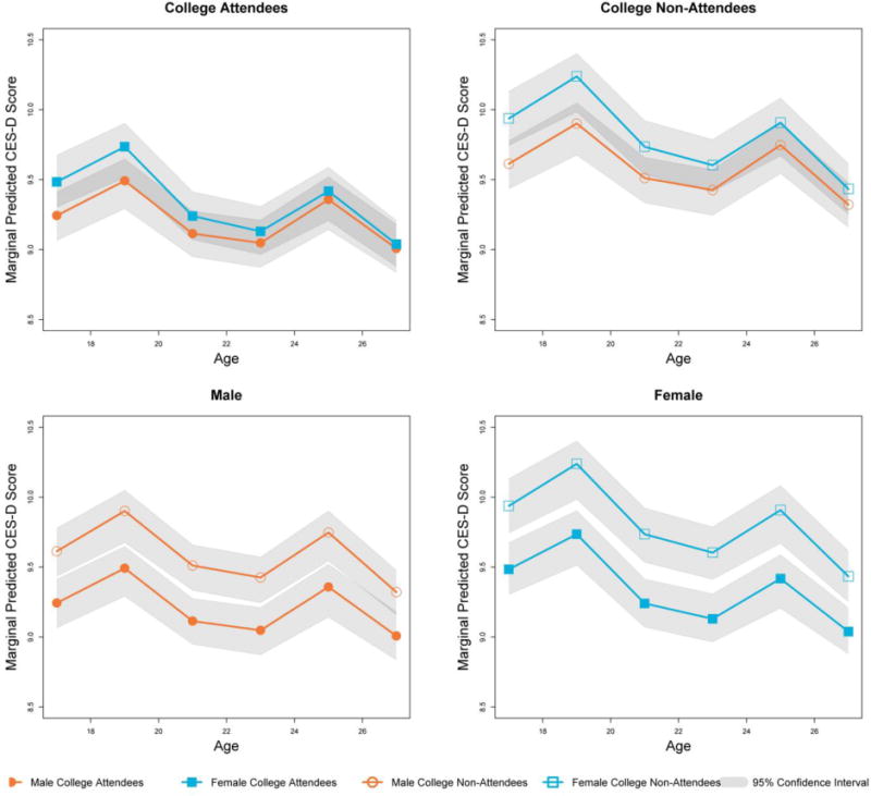
Empirical example 2: Marginal predicted values of the Center for Epidemiological Studies-Depression Scale for four subjects differing in gender and college attendance
Marginal trajectories predict the course of depressive symptoms based solely on the covariates of interest, and do not incorporate information about the individual values for the latent variables. Since the latent variables are unobserved, marginal predicted values truly represent what one would expect based only on the known information. However, for some purposes it is useful to incorporate inferred information about the latent variables when computing the predicted values. For the fitted GMM, the conditional predicted values in Equation (9) are obtained as
| (20) |
Here we display the “person fit” of the model for two cases from each class. For each class k, two cases two cases were selected at random among those with . Conditional predicted values were plotted against observed values, shown in Figure 5. Additionally, given the bootstrapping procedure described above, prediction intervals were generated using B = 2500 predicted values in order to approximate the uncertainty of the prediction. Across the six individuals, a few subjects (e.g., Subjects 321, 379, and 372) have at least one data point which lies far from the line of prediction; however, all individual data points are enclosed within the corresponding prediction intervals.
Figure 5.
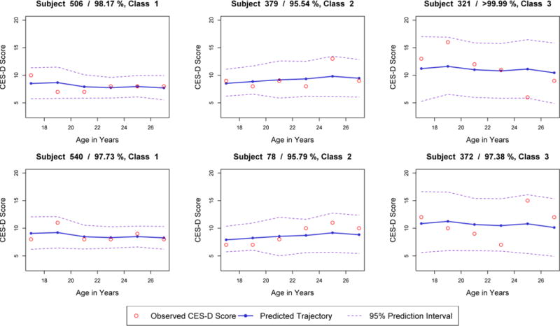
Empirical example 2: Conditional predicted values and observed values of the Center for Epidemiological Studies-Depression Scale for Six Subjects.
Visual examination of Figure 5 suggests varying levels of closeness between observed data points and the model-predicted values. The observed scores of some individuals appear to increase more or less rapidly than predicted, or change more erratically. Nevertheless, the observed values are within range that the model predicts should be observed, suggesting that the model provides reasonably good fit for these individuals. For other individuals, examination of plots such as these might suggest poor person fit, prompting the analyst to consider refinements to the model (e.g., the addition or subtraction of a trajectory class). The predicted and observed values for four such cases are shown in Figure 6; among cases with complete data, these cases are the four with the highest mean squared distance between the observed and predicted data points. Visual examination suggests that the depressive symptoms of some individuals (particularly Subjects 788 and 880) are characterized by a more systematic trend than the model is capturing.
Figure 6.
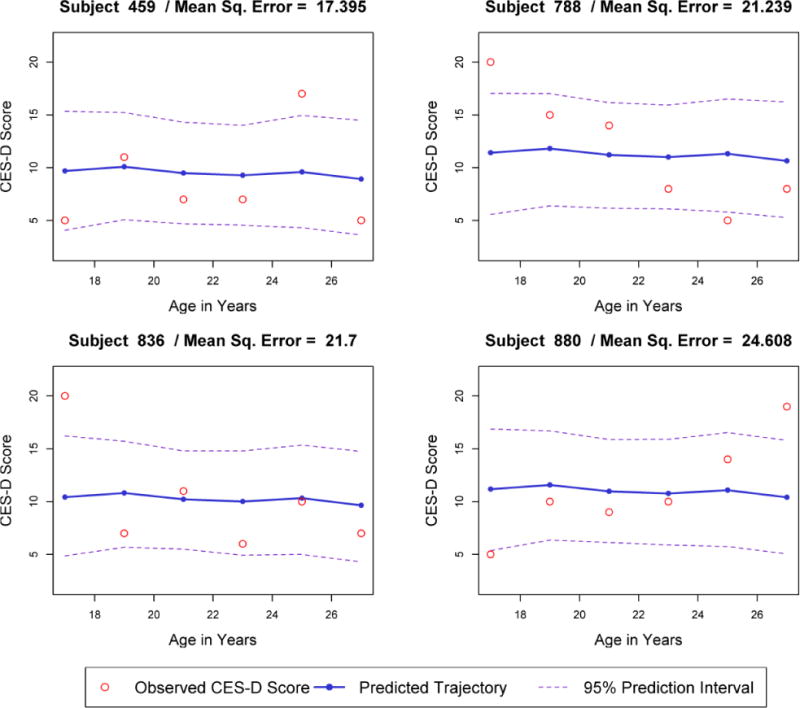
Empirical example 2: Conditional predicted values and observed values of the Center for Epidemiological Studies-Depression Scale for four subjects with poor model fit. specifically, our s of approximating uncertainty around predicted values using parametric bootstrapping (Efron and Tibshiran
In sum, marginal predicted values helped us to illustrate how we would expect individuals differing in their covariate values to differ in their trajectories of depression, averaging over the distributions of the unknown latent variables. In contrast, conditional predicted values allowed us to incorporate information about the latent variables to examine the predictions and fit of the model at the individual level.
Discussion
The current report explored a method for using mixture model results to make inferences about individuals, whether hypothetical or observed. We described and illustrated the use of both marginal and conditional predicted values. Additionally, a method for quantifying uncertainty around these predicted values was introduced. In the first empirical example, we explored the link between early marijuana use and subsequent non-medical use of prescription medications. In the second example, we used predicted values to examine the roles of gender and college attendance as potential risk factors for the maintenance of depressive symptoms in early adulthood, and we examined how well the model fit the observed data at the individual level.
Making individual predictions based on mixture models represents a break from the more common practice of using these models for the sole purpose of making inferences about latent sub-populations or the population as a whole. Computing and using predicted values for individuals is, however, a natural extension of methods used in the multilevel modeling (Afshartous and De Leeuw, 2005; Skrondal and Rabe-Hesketh, 2009). latent curve modeling (Preacher, Curran, and Bauer, 2006), and item response theory (Reise, 2000) frameworks. The current work builds upon these methods by showing how the results obtained from any mixture model – longitudinal or cross-sectional, with discrete indicators or continuous – can be used to obtain marginal and conditional individual-level predicted values. We have also discussed a method for quantifying the uncertainty around predicted values which is tailored to the unique challenges presented by mixture models. In particular, the algorithms we present for forming confidence intervals and prediction intervals explicitly model uncertainty in class membership, which is critical in making inferences from mixture model results (Wang, Brown, and Bandeen-Roche, 2005; Vermunt, 2010; Asparouhov and Muthén, 2016). Our use of parametric bootstrapping also avoids the potential intractability of analytical solutions for some models, for instance as might arise when specifying different distribution functions across classes (Mallick and Gelfand, 1994; Fang, Li, and Sun, 2005). As we previously discussed, this parametric boostrapping approach makes a number of assumptions, but there are reasons to believe that the intervals which result may be relatively robust so long as the fitted model provides a sufficient approximation to the data generating process. More research is needed to clarify this possibility.
In sum, mixture models allow for the modeling of increasingly complex relationships between variables, and our understanding of the substantive implications of the results can often be aided by computing and plotting the individual-level predicted values (whether for hypothetical or sampled individuals). Moreover, focusing on the predictions these models afford for specific individuals brings their application into greater alignment with a person-centered data analytic approach.
Acknowledgments
This work was supported by National Institutes of Health grants F31 DA040334 (Fellow: Veronica Cole) and R01 DA034636 (PI: Daniel Bauer). The content is solely the responsibility of the authors and does not represent the official views of the National Institute on Drug Abuse or the National Institutes of Health. The authors would like to thank Danielle Dean and Jolynn Pek for helpful comments on this paper.
Footnotes
Note that here and throughout the text the term marginal is applied when marginalizing with respect to the latent variables, though the expression remains conditional on the observed exogenous covariates.
References
- Afshartous D, de Leeuw J. Prediction in multilevel models. Journal of Educational and Behavioral Statistics. 2005;30(2):109–139. [Google Scholar]
- Arminger G, Schoenberg RJ. Pseudo maximum likelihood estimation and a test for misspecification in mean and covariance structure models. Psychometrika. 1989;54(3):409–425. [Google Scholar]
- Asparouhov T, Muthén B. Structural equation models and mixture models with continuous nonnormal skewed distributions. Structural Equation Modeling: A Multidisciplinary Journal. 2016;23(1):1–19. [Google Scholar]
- Bauer DJ, Baldasaro RE, Gottfredson NC. Diagnostic procedures for detecting nonlinear relationships between latent variables. Structural Equation Modeling: A Multidisciplinary Journal. 2012;19(2):157–177. [Google Scholar]
- Bauer DJ, Curran PJ. Distributional assumptions of growth mixture models: implications for overextraction of latent trajectory classes. Psychological Methods. 2003;8(3):338. doi: 10.1037/1082-989X.8.3.338. [DOI] [PubMed] [Google Scholar]
- Bauer DJ, Curran PJ. The integration of continuous and discrete latent variable models: potential problems and promising opportunities. Psychological Methods. 2004;9(1):3. doi: 10.1037/1082-989X.9.1.3. [DOI] [PubMed] [Google Scholar]
- Bauer DJ, Shanahan MJ. Modeling complex interations: person-centered and variable-centered approaches. In: Little TD, Bovaird JA, Card NA, editors. Modeling Contextual Effects in Longitudinal Studies. Mahwah, NJ: Lawrence Erlbaum Associates; 2007. pp. 255–284. [Google Scholar]
- Bergman LR, Magnusson D. A person-oriented approach in research on developmental psychopathology. Development and Psychopathology. 1997;9(2):291–319. doi: 10.1017/s095457949700206x. [DOI] [PubMed] [Google Scholar]
- Blanco C, Okuda M, Wright C, Hasin DS, Grant BF, Liu SM, Olfson M. Mental health of college students and their non–college-attending peers: Results from the national epidemiologic study on alcohol and related conditions. Archives of General Psychiatry. 2008;65(12):1429–1437. doi: 10.1001/archpsyc.65.12.1429. [DOI] [PMC free article] [PubMed] [Google Scholar]
- Bock RD, Aitkin M. Marginal maximum likelihood estimation of item parameters: Application of an EM algorithm. Psychometrika. 1981;46(4):443–459. [Google Scholar]
- Bolck A, Croon M, Hagenaars J. Estimating latent structure models with categorical variables: One-step versus three-step estimators. Political Analysis. 2004;12(1):3–27. [Google Scholar]
- Boyd CJ, McCabe SE, Cranford JA, Young A. Adolescents’ motivations to abuse prescription medications. Pediatrics. 2006;118(6):2472–2480. doi: 10.1542/peds.2006-1644. [DOI] [PMC free article] [PubMed] [Google Scholar]
- Browne MW, Arminger G. Specification and estimation of mean-and covariance-structure models. In: Arminger G, Clogg CC, Sobel ME, editors. Handbook of statistical modeling for the social and behavioral sciences. New York: Plenum; 1995. pp. 185–249. [Google Scholar]
- Compton WM, Volkow ND. Abuse of prescription drugs and the risk of addiction. Drug and Alcohol Dependence. 2006;83:S4–S7. doi: 10.1016/j.drugalcdep.2005.10.020. [DOI] [PubMed] [Google Scholar]
- Conijn JM, Emons WH, De Jong K, Sijtsma K. Detecting and Explaining Aberrant Responding to the Outcome Questionnaire–45. Assessment. 2015;22:513–524. doi: 10.1177/1073191114560882. [DOI] [PubMed] [Google Scholar]
- Curran PJ, Bauer DJ, Willoughby MT. Testing main effects and interactions in latent curve analysis. Psychological Methods. 2004;9(2):220. doi: 10.1037/1082-989X.9.2.220. [DOI] [PubMed] [Google Scholar]
- Davison AC, Hinkley DV. Bootstrap methods and their application. Vol. 1. Cambridge: Cambridge University Press; 1997. [Google Scholar]
- Dean DO, Bauer DJ, Shanahan MJ. A discrete-time Multiple Event Process Survival Mixture (MEPSUM) model. Psychological Methods. 2014;19(2):251. doi: 10.1037/a0034281. [DOI] [PMC free article] [PubMed] [Google Scholar]
- Dean DO, Cole V, Bauer DJ. Delineating prototypical patterns of substance use initiations over time. Addiction. 2015;110(4):585–594. doi: 10.1111/add.12816. [DOI] [PubMed] [Google Scholar]
- Dempster AP, Laird NM, Rubin DB. Maximum likelihood from incomplete data via the EM algorithm. Journal of the royal statistical society. Series B (methodological) 1977;34:1–38. [Google Scholar]
- Depaoli S. Mixture class recovery in GMM under varying degrees of class separation: Frequentist versus Bayesian estimation. Psychological Methods. 2013;18(2):186. doi: 10.1037/a0031609. [DOI] [PubMed] [Google Scholar]
- deRoon-Cassini TA, Mancini AD, Rusch MD, Bonanno GA. Psychopathology and resilience following traumatic injury: a latent growth mixture model analysis. Rehabilitation Psychology. 2010;55(1):1. doi: 10.1037/a0018601. [DOI] [PubMed] [Google Scholar]
- Efron B, Hinkley DV. Assessing the accuracy of the maximum likelihood estimator: Observed versus expected Fisher information. Biometrika. 1978;65(3):457–483. [Google Scholar]
- Efron B, Tibshirani RJ. An introduction to thebootstrap. Monographs on Statistics and Applied Probability. 1993:57. [Google Scholar]
- Eliason SR. Maximum likelihood estimation: Logic and practice. Vol. 96. Thousand Oaks, CA: Sage Publications; 1993. [Google Scholar]
- Fang HB, Li G, Sun J. Maximum Likelihood Estimation in a Semiparametric Logistic/Proportional-Hazards Mixture Model. Scandinavian Journal of Statistics. 2005;32(1):59–75. [Google Scholar]
- Gfroerer JC, Greenblatt JC, Wright DA. Substance use in the US college-age population: differences according to educational status and living arrangement. American Journal of Public Health. 1997;87(1):62–65. doi: 10.2105/ajph.87.1.62. [DOI] [PMC free article] [PubMed] [Google Scholar]
- Gibson WA. Three multivariate models: Factor analysis, latent structure analysis, and latent profile analysis. Psychometrika. 1959;24(3):229–252. [Google Scholar]
- Gottfredson NC, Bauer DJ, Baldwin SA, Okiishi J. Using a shared parameter mixture model to estimate change during treatment when treatment termination is related to recovery speed. Journal of Consulting and Clinical Psychology. 2014;82:813–827. doi: 10.1037/a0034831. [DOI] [PMC free article] [PubMed] [Google Scholar]
- Grice JW. Computing and evaluating factor scores. Psychological methods. 2001;6(4):430–450. [PubMed] [Google Scholar]
- Huang GH, Bandeen-Roche K. Building an identifiable latent class model with covariate effects on underlying and measured variables. Psychometrika. 2004;69(1):5–32. [Google Scholar]
- Hoeksma JB, Kelderman H. On growth curves and mixture models. Infant and Child Development. 2006;15(6):627–634. [Google Scholar]
- Huber PJ. Proceedings of the Fifth Berkeley Symposium on Mathematical Statistics and Probability. Vol. 1. Berkeley, CA: University of California Press; 1967. The behavior of maximum likelihood estimates under nonstandard conditions; pp. 221–233. [Google Scholar]
- Kandel DB. Stages and pathways of drug involvement: Examining the gateway hypothesis. Cambridge: Cambridge University Press; 2002. [Google Scholar]
- Kelava A, Nagengast B, Brandt H. A Nonlinear Structural Equation Mixture Modeling Approach for Nonnormally Distributed Latent Predictor Variables. Structural Equation Modeling: A Multidisciplinary Journal. 2014;21(3):468–481. [Google Scholar]
- Kovacevic M, Huang R, You Y. Bootstrapping for variance estimation in multi-level models fitted to survey data. ASA Proceedings of the Survey Research Methods Section. 2006:3260–3269. [Google Scholar]
- Kutner MH, Nachtsheim C, Neter J. Applied linear regression models. Chicago, IL: McGraw-Hill/Irwin; 2004. [Google Scholar]
- Lanza ST, Tan X, Bray BC. Latent class analysis with distal outcomes: A flexible model-based approach. Structural Equation Modeling: a Multidisciplinary Journal. 2013;20(1):1–26. doi: 10.1080/10705511.2013.742377. [DOI] [PMC free article] [PubMed] [Google Scholar]
- Laursen BP, Hoff E. Person-centered and variable-centered approaches to longitudinal data. Merrill-Palmer Quarterly. 2006;52(3):377–389. [Google Scholar]
- Lazarsfeld PF, Henry NW. Latent structure analysis. Boston: Houghton Mifflin; 1968. [Google Scholar]
- Louis TA. Finding the observed information matrix when using the EM algorithm. Journal of the Royal Statistical Society. Series B (Methodological) 1982;44:226–233. [Google Scholar]
- Mallick BK, Gelfand AE. Generalized linear models with unknown link functions. Biometrika. 1994;81(2):237–245. [Google Scholar]
- McLachlan G, Peel D. Finite mixture models. John Wiley & Sons; 2000. [Google Scholar]
- Meredith W, Tisak J. Latent curve analysis. Psychometrika. 1990;55(1):107–122. [Google Scholar]
- Morin AJ, Maïano C, Nagengast B, Marsh HW, Morizot J, Janosz M. General growth mixture analysis of adolescents’ developmental trajectories of anxiety: the impact of untested invariance assumptions on substantive interpretations. Structural Equation Modeling: A Multidisciplinary Journal. 2011;18(4):613–648. [Google Scholar]
- Muthén B, Muthén LK. Integrating person-centered and variable-centered analyses: Growth mixture modeling with latent trajectory classes. Alcoholism: Clinical and Experimental Research. 2000;24(6):882–891. [PubMed] [Google Scholar]
- Muthén B, Shedden K. Finite mixture modeling with mixture outcomes using the EM algorithm. Biometrics. 1999;55(2):463–469. doi: 10.1111/j.0006-341x.1999.00463.x. [DOI] [PubMed] [Google Scholar]
- Nagin D. Group-based modeling of development. Cambridge, MA: Harvard University Press; 2005. [Google Scholar]
- Nagin DS. Analyzing developmental trajectories: a semiparametric, group-based approach. Psychological Methods. 1999;4(2):139. doi: 10.1037/1082-989x.6.1.18. [DOI] [PubMed] [Google Scholar]
- Nagin DS, Tremblay RE. Developmental trajectory groups: Fact or a useful statistical fiction? Criminology. 2005;43:837–904. [Google Scholar]
- Pek J, Chalmers RP, Kok BE, Losardo D. Visualizing confidence bands for semiparametrically estimated nonlinear relations among latent variables. Journal of Educational and Behavioral Statistics 2015 [Google Scholar]
- Pek J, Losardo D, Bauer DJ. Confidence intervals for a semiparametric approach to modeling nonlinear relations among latent variables. Structural Equation Modeling: A Multidisciplinary Journal. 2011;18(4):537–553. [Google Scholar]
- Preacher KJ, Curran PJ, Bauer DJ. Computational tools for probing interactions in multiple linear regression, multilevel modeling, and latent curve analysis. Journal of Educational and Behavioral Statistics. 2006;31(4):437–448. [Google Scholar]
- Preacher KJ, Selig JP. Advantages of Monte Carlo confidence intervals for indirect effects. Communication Methods and Measures. 2012;6(2):77–98. [Google Scholar]
- Ram N, Grimm KJ. Methods and measures: Growth mixture modeling: A method for identifying differences in longitudinal change among unobserved groups. International Journal of Behavioral Development. 2009;33(6):565–576. doi: 10.1177/0165025409343765. [DOI] [PMC free article] [PubMed] [Google Scholar]
- Raudenbush SW. Comparing personal trajectories and drawing causal inferences from longitudinal data. Annual review of psychology. 2001;52(1):501–525. doi: 10.1146/annurev.psych.52.1.501. [DOI] [PubMed] [Google Scholar]
- Reise SP. Using multilevel logistic regression to evaluate person-fit in IRT models. Multivariate Behavioral Research. 2000;35(4):543–568. doi: 10.1207/S15327906MBR3504_06. [DOI] [PubMed] [Google Scholar]
- Robins LN, Darvish HS, Murphy GE. The long-term outcome for adolescent drug users: a follow-up study of 76 users and 146 nonusers. In: Zubin J, Freedman AM, editors. Proceedings of the annual meeting of the American Psychopathological Association. Vol. 59. New York: Grune and Stratton; 1970. pp. 159–178. [PubMed] [Google Scholar]
- Satorra A. Robustness issues in structural equation modeling: A review of recent developments. Quality and Quantity. 1990;24(4):367–386. [Google Scholar]
- Satorra A, Bentler PM. Corrections to test statistics and standard errors in covariance structure analysis. In: von Eye A, Clogg CC, editors. Latent variables analysis: Applications for developmental research. Thousand Oaks, CA: Sage; 1994. pp. 399–419. [Google Scholar]
- Schwarz G. Estimating the dimension of a model. The Annals of Statistics. 1978;6(2):461–464. [Google Scholar]
- Skrondal A, Laake P. Regression among factor scores. Psychometrika. 2001;66(4):563–575. [Google Scholar]
- Skrondal A, Rabe-Hesketh S. Prediction in multilevel generalized linear models. Journal of the Royal Statistical Society: Series A (Statistics in Society) 2009;172(3):659–687. [Google Scholar]
- Sterba SK, Bauer DJ. Matching method with theory in person-oriented developmental psychopathology research. Development and Psychopathology. 2010;22:239–254. doi: 10.1017/S0954579410000015. [DOI] [PubMed] [Google Scholar]
- Sterba SK, Bauer DJ. Predictions of individual change recovered with latent class or random coefficient growth models. Structural Equation Modeling: A Multidisciplinary Journal. 2014;21(3):342–360. [Google Scholar]
- Titterington DM, Smith AF, Makov UE. Statistical analysis of finite mixture distributions. Vol. 7. New York: Wiley; 1985. [Google Scholar]
- Tucker LR. Relations of factor score estimates to their use. Psychometrika. 1971;36(4):427–436. [Google Scholar]
- Tueller S, Lubke G. Evaluation of structural equation mixture models: Parameter estimates and correct class assignment. Structural Equation Modeling. 2010;17(2):165–192. doi: 10.1080/10705511003659318. [DOI] [PMC free article] [PubMed] [Google Scholar]
- van der Leeden R, Meijer E, Busing FM. Resampling multilevel models. In: deLeeuw J, Meijer E, editors. Handbook of multilevel analysis. New York: Springer; 2008. pp. 401–433. [Google Scholar]
- Van Horn ML, Smith J, Fagan AA, Jaki T, Feaster DJ, Masyn K, Hawkins D, Howe G. Not quite normal: Consequences of violating the assumption of normality in regression mixture models. Structural equation modeling: a multidisciplinary journal. 2012;19(2):227–249. doi: 10.1080/10705511.2012.659622. [DOI] [PMC free article] [PubMed] [Google Scholar]
- Vermunt JK. Latent class modeling with covariates: Two improved three-step approaches. Political Analysis. 2010;18(4):450–469. [Google Scholar]
- Wang CP, Brown CH, Bandeen-Roche K. Residual diagnostics for growth mixture models: Examining the impact of a preventive intervention on multiple trajectories of aggressive behavior. Journal of the American Statistical Association. 2005;100(471):1054–1076. [Google Scholar]
- White H. Maximum likelihood estimation of misspecified models. Econometrica. 1982;50:1–25. [Google Scholar]
- Wiesner M, Windle M. Assessing covariates of adolescent delinquency trajectories: A latent growth mixture modeling approach. Journal of Youth and Adolescence. 2004;33(5):431–442. [Google Scholar]
- Woods CM, Oltmanns TF, Turkheimer E. Detection of aberrant responding on a personality scale in a military sample: An application of evaluating person fit with two-level logistic regression. Psychological assessment. 2008;20(2):159. doi: 10.1037/1040-3590.20.2.159. [DOI] [PMC free article] [PubMed] [Google Scholar]
- Yuan KH, Bentler PM. Mean and covariance structure analysis: Theoretical and practical improvements. Journal of the American Statistical Association. 1997;92:767–774. [Google Scholar]
- Yung YF, Bentler PM. Bootstrapping techniques in analysis of mean and covariance structures. In: Marcoulides GA, Schumacker RE, editors. Advanced structural equation modeling: Issues and techniques. Mahwah, NJ: Lawrence Erlbaum Associates, Inc; 1996. pp. 195–226. [Google Scholar]