A simple method to control over-alignment in the MAFFT multiple sequence alignment program

Abstract

Motivation: We present a new feature of the MAFFT multiple alignment program for suppressing over-alignment (aligning unrelated segments). Conventional MAFFT is highly sensitive in aligning conserved regions in remote homologs, but the risk of over-alignment is recently becoming greater, as low-quality or noisy sequences are increasing in protein sequence databases, due, for example, to sequencing errors and difficulty in gene prediction.

Results: The proposed method utilizes a variable scoring matrix for different pairs of sequences (or groups) in a single multiple sequence alignment, based on the global similarity of each pair. This method significantly increases the correctly gapped sites in real examples and in simulations under various conditions. Regarding sensitivity, the effect of the proposed method is slightly negative in real protein-based benchmarks, and mostly neutral in simulation-based benchmarks. This approach is based on natural biological reasoning and should be compatible with many methods based on dynamic programming for multiple sequence alignment.

Availability and implementation: The new feature is available in MAFFT versions 7.263 and higher. http://mafft.cbrc.jp/alignment/software/

Contact: katoh@ifrec.osaka-u.ac.jp

Supplementary information: Supplementary data are available at Bioinformatics online.

1 Introduction

Many comparative analyses of biological sequences utilize multiple sequence alignment (MSA), and the quality of an MSA can affect the results of downstream analyses. Therefore, even incremental improvements in MSA quality can have wide-ranging effects. One area in MSA technology that can potentially be improved is robustness against noise in sequence data.

As a result of large-scale sequencing projects, we now have access to many amino acid and nucleotide sequences from widely divergent organisms. Unfortunately, the quality of the sequences is not always high, partly due to limitations in sequencing technologies. Moreover, at the amino acid sequence level, a number of errors can be introduced due to difficulty in gene prediction (Brent, 2005; Gotoh et al., 2014; Nagy and Patthy, 2013; Yandell and Ence, 2012). With incorrect reading frames, unrelated amino acid segments can appear in a set of homologous sequences. Even if such errors could be completely excluded, splice variants of a gene can be included in an MSA of a Eukaryotic gene family. Another source of difficulty is when small structural domains are surrounded by intrinsically disordered or low-complexity regions (Thompson et al., 2011). Thus, the existence of unrelated segments, or noise, in an MSA is common, especially in large-scale analyses of amino acid sequences, for which human inspection is difficult. Therefore robustness in such situations is an important feature for any MSA method used for large-scale analysis.

Most MSA methods assume that the input sequences are all homologous. When the input sequences have unrelated segments, these segments often end up being aligned. This results in ‘over-alignment’; i.e. sites that are aligned but are, in fact, non-homologous (Blackburne and Whelan, 2012a; Schwartz and Pachter, 2007). Some MSA methods, including PRANK and BAli-Phy, are aware of this problem (Bradley et al., 2009; Löytynoja and Goldman, 2005, 2008; Redelings, 2014; Suchard and Redelings, 2006). However, these methods are not ranked highly in standard benchmarks based on protein structural alignments (Sievers et al., 2011). This is not surprising because the standard criterion is essentially based on sensitivity, a consequence of which is that the over-alignment problem is not taken into account.

Methods such as PRANK and BAli-Phy usually utilize simulated input to test alignment accuracy. Simulation-based benchmarks generally have a limitation in that the simulation setting is inevitably oversimplified and the applicability to real-world situations is unclear. On the other hand, the use of real data is problematic, when considering over-alignment, due to the arbitrariness of reference alignments (Edgar, 2010). More specifically, structural alignments can only provide information about sites that are structurally conserved, not sites that are unrelated. In simulation-based benchmarks that take into consideration over-alignment, PRANK and BAli-Phy consistently outperform other methods (Löytynoja and Goldman, 2008; Redelings, 2014). Thus there is a discrepancy between benchmarks based on real data and simulated data. To assess the over-alignment problem, both types of benchmarks are necessary.

Here, we describe a simple method to control over-alignment directly and flexibly in a protein MSA. In brief, the proposed method utilizes agreement between the local segments and the entire sequence to determine which residues should be aligned; if there is a dissimilar segment in a globally highly similar pair of sequences, the dissimilar segment is gapped. This is accomplished by using a variable scoring matrix (VSM) that adapts to the global similarity between a pair of sequences (or groups) within an MSA given a single additional parameter that controls the risk of over-alignment. This is not a novel idea since it is based on a combination of two techniques known for more than 20 years: (i) adjusting the overall average of a scoring matrix (Vingron and Waterman, 1994) by rescaling the matrix according to the similarity of the pair of sequences or groups to be aligned and (ii) use of different scoring matrices in an MSA, as originally proposed in ClustalW (Thompson et al., 1994), but probably not inherited by Clustal Omega (Sievers et al., 2011). We have implemented the VSM technique in the MAFFT program (Katoh et al., 2002; Katoh and Standley, 2013), which is one of the most sensitive methods in terms of standard criteria (Sievers et al., 2011; Thompson et al., 2011).

2 Methods

Protein sequence alignment by dynamic programming (DP) (Needleman and Wunsch, 1970) uses a scoring matrix with 20 × 20 elements (e.g. BLOSUM (Henikoff and Henikoff, 1992), GCB (Gonnet et al., 1992), PAM (Dayhoff et al., 1978), JTT (Jones et al., 1992)). MAFFT uses BLOSUM62 by default. DP gives the optimal alignment of two sequences by maximizing the alignment score, defined as the summation of the scores of aligned pairs and gap costs. Here we use the gap open cost (<0) only.

We use a modified matrix M(A, B) in which a positive value a is subtracted from all the elements of the scoring matrix.

$$M(A,B)=M_{\text{orig}}(A,B)-a(a>0),$$ (1)

where A and B are amino acids. The original scoring matrix $M_{\text{orig}}(A,B)$ is normalized such that ${\displaystyle \sum f_A}{M}_{\text{orig}}(A,A)=1$ and ${\displaystyle \sum {\displaystyle \sum f_A}}{f}_B{M}_{\text{orig}}(A,B)=0$, in the case of MAFFT, where f_A and f_B are the frequencies of amino acids A and B, respectively.

When a is close to one, some of the diagonal elements have negative values. In such a case, there can be situations where the optimal solution is to insert gaps even for identical sequences,

This occurs for the following reason; the score for the match of S-S, A-A and T-T are 0.815, 0.815 and 0.924, respectively, in the BLOSUM62 matrix normalized as above. In an unrealistic case of a = 1, the score for matching the segment SATSATSAT, –1.338, is negative. As a result, depending on gap cost, the above alignment can have a better score than the gap-less alignment, which has a ‘cost’ of –1.338 for matching the segment when a = 1. Although this example is an extreme one, it indicates a possibility that the segments with weak or ambiguous similarity are not aligned if a positive value, a, is subtracted from the scoring matrix. Inversely, if a positive value is added to the scoring matrix, even non-similar residues are matched. These effects were discussed in Vingron and Waterman (1994).

An alignment with a high a value (close to one), where low-similarity segments tend not to be aligned, is preferable when the expected evolutionary distance between the sequences is small. Imagine a case where some dissimilar segments are found in a set of closely-related sequences. It is reasonable to infer that these segments were inserted due to some unusual factors, such as sequencing errors or alternative splicing, and thus should be gapped. Meanwhile, a low a value (close to zero) is useful when the evolutionary distance between the sequences is expected to be large, where low-similarity segments have to be aligned.

Thus we should use a large a value for closely-related sequences and a small or zero a value for distantly-related sequences. The value of a can be interpreted as the ‘lowest similarity level to align’, ranging from zero to one, where zero corresponds to unrelated sequences and one corresponds to complete match. In the case of global alignment, we can estimate the expected similarity level, or evolutionary distance d, of the entire input sequences. It is natural to use large a for a pair with small d, and to use small a for a pair with large d. In the case of MAFFT, the distance d_ij between sequences i and j is estimated as a value between zero and one, $d_{ij}=1-(t_{ij}/\min \hspace{0.17em}(t_{ii},t_{jj})),$ where t_ij is the alignment score between sequences i and j. So, we use a variable a(d), depending on d and a new parameter, $a_{\text{max}}$, to dynamically generate a variable scoring matrix (VSM) according to the distance d between the pair to be aligned, as

$$M(A,B,d)=M_{\text{orig}}(A,B)-a(d)$$ (2)

$$\begin{array}{ccc}a(d)=& a_{\text{max}}-d& \text{if\hspace{0.17em}\hspace{0.17em}}{a}_{\text{max}}>d\\ a(d)=& 0& \text{Otherwise}.\end{array}$$

As discussed above, $a()$=1 is unrealistic even in the case of d = 0, and thus a margin is necessary. We can interpret $1-a_{\text{max}}$ as such a margin.

In their pioneering work, the authors of ClustalW (Thompson et al., 1994) used different scoring matrices according to similarity level of the groups (or sequences) to be aligned. This method uses the BLOSUM 30, 45, 62 and 80 matrices. This strategy (which uses multiple scoring matrices for different similarities and referred to as ‘MSM’ hereafter) seems to be more natural than VSM (a single original matrix is modified based on distance information). A detailed comparison between these two strategies is given at the beginning of Section 3.

2.1 Determination of $a_{\text{max}}$

The proposed method has an additional parameter, $a_{\text{max}}$. As discussed above, too large an $a_{\text{max}}$ value is expected to result in low-quality alignments. This parameter has to be empirically determined (see Section 3).

2.2 Implementation

The above modification was made in the DP calculations of the G-INS-i option of MAFFT. The calculation procedure of this option consists of three stages, all-to-all comparison, progressive alignment and iterative refinement. Modification in each stage is described in the next paragraphs. We consider the case of amino acid sequence with a VSM $M(A,B,d)$ derived from the BLOSU62 matrix, where A and B are amino acids and d is evolutionary distance between groups or sequences to be compared.

2.3 All-to-all comparison

The initial step of MAFFT-G-INS-i is the estimation of a guide tree. All-to-all DP calculation is performed. To include the above idea into this calculation, the DP calculation is repeated twice for each pair. First, a normal DP calculation is performed using a standard scoring matrix, to determine the evolutionary distance d between the pair. Second, the alignment is re-calculated using a VSM with d. These pairwise alignments are used to compute the objective score similar to COFFEE (Notredame et al., 1998) in the later stages.

2.4 Progressive method

The implementation of the above idea in the progressive alignment (Feng and Doolittle, 1987; Higgins and Sharp, 1988) stage is quite easy. MAFFT uses a guide tree that assumes that all the lineages have the same evolutionary rate (the distances from an internal node to its descendant termini are all constant). In each step of the group-to-group alignment calculation, we can estimate the expected evolutionary distance d_IJ between the groups I and J as 2 × the branch length from the node to its descendant termini. In any step in the progressive calculation, the distance between sequences is identical in any sequence pair involved in the step. Therefore the calculation can be done by just replacing the original scoring matrix with a VSM.

Formally, in the DP matrix, the score $S(I,J,x,y)$ for the match of the xth site in group I and the yth site in group J is calculated as

$$S(I,J,x,y)={\displaystyle \sum _{i\in I}{\displaystyle \sum _{j\in J}{w}_i}}{w}_{j}M(A_{ix},B_{jy},d_{ij}),$$ (3)

where A_ix is the xth site in the ith sequence in group I, and w_i is the weight for sequence i, and B_jy is defined similarly. To reduce the computational cost, $S(,,,)$ is usually computed by comparing two weight matrices, $W_I()$ and $W_J()$.

$$S(I,J,x,y)={\displaystyle \sum _{m=1}^{20}{\displaystyle \sum _{n=1}^{20}M}}(m,n,d_{IJ})W_I(m,x)W_J(n,y).$$ (4)

Note that d_ij is identical (denoted as d_IJ) for any sequence pairs across group I and J, in the case of progressive alignment. The weight matrix $W_I()$ is calculated as

$$\begin{array}{cc}{W}_I(m,x)={\displaystyle \sum _{i\in I}{w}_i}g(m,i,x)& \text{if\hspace{0.17em}}m=A_{ix},g(m,i,x)=1;\\ & \text{otherwise\hspace{0.17em}}g(m,i,x)=0,\end{array}$$ (5)

where w_i is the weight for sequence i. $W_J(n,y)$ is calculated similarly. Thus the only difference is in the use of $M(A,B,d)$ instead of $M_{\text{orig}}(A,B)$.

2.5 Iterative refinement method

In the iterative refinement step (Barton and Sternberg, 1987; Berger and Munson, 1991; Gotoh, 1996), the initial alignment is divided into two groups, I and J, and then the groups are re-aligned. In this case, too, the DP matrix $S()$ is constructed as in Eq. 3. However, the above group-to-group alignment technique cannot directly be applied in this case, because the distance d_ij is not identical for sequence pairs across group I and J. For this case, the distance d_ij is digitalized into several (10 in our current implementation) distance classes, and a pair of weight matrices is prepared for each distance class, to compute an approximate DP matrix $S\prime ()$.

$$S\prime (I,J,x,y)={\displaystyle \sum _{c=1}^{10}{\displaystyle \sum _{m=1}^{20}{\displaystyle \sum _{n=1}^{20}M}}}(m,n,D(c))W_I(m,x,c,J)W_J(n,y,c,I)$$ (6)

$$\begin{array}{cc}& D(c)=0.05,0.15,\dots 0.95\\ & W_I(m,x,c,J)={\displaystyle \sum _{i\in I}{w}_i}g(m,i,x,c,J)\end{array}$$

$$\begin{array}{cc}\text{if\hspace{0.17em}}{A}_{ix}=m\text{\hspace{0.17em}and\hspace{0.17em}}\exists j\in J(d_{ij}\sim D(c)),\text{then\hspace{0.17em}}g(m,i,x,c,J)=& 1\\ \text{otherwise\hspace{0.17em}}g(m,i,x,c,J)=0.\end{array}$$

$W_J(n,y,c,I)$ is calculated similarly. Note that group I’s weight matrix, $W_I(m,x,c,J)$, depends on the counterpart, group J, as well as group I itself. So the weight matrices have to be recalculated for every pair of groups. $S\prime ()$ approaches $S()$ when the number of the distance classes increases.

3 Results

We described the variable scoring matrix (VSM) technique, which uses a single scoring matrix $M_{\text{orig}}(,)$ with a variable a, in Methods. There is another (possibly more natural) strategy, the use of multiple scoring matrices (MSM) such as the BLOSUM series, each of which is for a specific similarity level. This technique was originally used in ClustalW (Thompson et al., 1994). We compared the effect of VSM and MSM using a simple pairwise alignment with four distinct regions,

where the two sequences are identical in the first and fourth regions, but unrelated in the second and third regions. The above alignment should be correct, but the second and third regions are often confusingly aligned with a number of short gaps, which is a typical case of over-alignment. We created this type of paired artificial amino acid sequences (length of each region = 100) and computed the optimum pairwise alignments, changing scoring matrix (BLOSUM45 to BLOSUM100 and JTT PAM200 to JTT PAM1) and the a value, independently. For the JTT series, PAM1 transition probability matrix was multiplied x times to generate PAMx transition probability matrices $P(A\to B,x)$, from which log-odds scoring matrices $M(A,B,x)$ were derived in the standard manner (Dayhoff et al., 1978), $M(A,B,x)=\log \hspace{0.17em}\hspace{0.17em}{f}_{A}P(A\to B,x)/f_A{f}_B\}$, where f_A and f_B are frequencies of amino acids A and B, respectively. The scoring matrices were not normalized unlike the normal calculation of MAFFT, in order to directly test the effect of the matrices. We tried three different gap costs, 0.5, 1.5 and 2.5× (the average of the diagonal elements of the original scoring matrix). The proportion of correctly placed gaps over the number of gaps in the true alignment was scored for each parameter set. Average scores with 100 replications are shown in Figure 1.

Fig. 1.

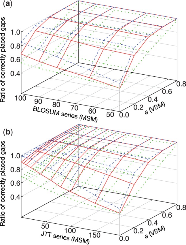
Comparison between MSM and VSM for (a) the BLOSUM series and (b) the JTT series. Blue dashed lines, red solid lines and green dotted lines correspond to the gap cost values of 2.5, 1.5 and 0.5× (the average of the diagonal elements of the original scoring matrix), respectively. The default gap cost of MAFFT is 1.53 in this scale and thus close to red

In the case of BLOSUM-MSM (the plots at a = 0.0 in Fig. 1a), a moderate effect of changing matrices was observed; by changing BLOSUM45 (for remote homologs) to BLOSUM100 (for close homologs), the average score increased from 0.441 to 0.679 in the red solid line. The effect of VSM (changing a) was clearly larger; the average score increased from 0.441 to 0.999 in the red solid line for BLOSUM45. The effect of VSM was also large for BLOSUM62 (0.515 → 0.999). The reason for the limited effect of BLOSUM-MSM is probably that BLOSUMx is built from blocks with identity of no more than x%. This means that distantly-related sequences are included even in the calculation of BLOSUM90 and 100.

JTT-MSM (Fig. 1b) was more effective (0.422 → 0.904 (red solid line) and 0.484 → 0.990 (blue dashed line) at a = 0.0) than BLOSUM-MSM. The JTT PAMx matrix is based on the extrapolation of a transition probability matrix of a closely-related pair. Consequently, the distantly-related pairs are not included in the calculation when x is small. This is probably the reason why JTT-MSM outperformed BLOSUM-MSM in this test. For the same reason, however, empirical matrices directly based on remote homologs are naturally preferable to extrapolated matrices for aligning distantly-related sequences. It is still unclear why JTT-VSM slightly outperformed JTT-MSM.

We compared several matrices in the above test using ‘expected ratio’ E, defined as the ratio of expected score (Henikoff and Henikoff, 1992) over the the average of diagonal elements (expected score for the alignment of identical sequences), $E(M(,))={\displaystyle \sum {\displaystyle \sum f_A}}{f}_{B}M(A,B)/{\displaystyle \sum f_A}M(A,A),$ where $M(,)$ is a scoring matrix and f_A and f_B are the frequencies of amino acids A and B, respectively. The actual values of $E(\text{JTT\hspace{0.17em}PAM1}),E(\text{JTT\hspace{0.17em}PAM200}),E(\text{BLOSUM100})$ and $E(\text{BLOSUM45})$ are –1.684, –0.184, –0.322 and –0.130, respectively, when assuming standard amino acid frequencies of the JTT model. The performance in avoiding over-alignment is JTT PAM1 > BLOSUM100 > BLOSUM45 ∼ JTT PAM200. This order is as theoretically expected and was confirmed in the above test. Thus E may be useful for predicting the behavior of a scoring matrix for this type of over-alignment before performing the actual calculation.

In the actual implementation of MAFFT, the scoring matrix is normalized such that the average of all elements (expected score) is zero, as noted in Methods. The modification with a is applied to this normalized matrix (Eq. 1). In this scoring scheme, E is always zero before subtracting a (the effect of MSM is cancelled), and then determined exclusively by a; $E=-a/(1-a)$. In the case of a = 0.8, for example, E=–4.0 independently of the selection of scoring matrix. In the subsequent parts of this report, we examine the effects and possible side effects of VSM in this scoring scheme with BLOSUM62, using actual data and more realistic simulations.

3.1 Examples

Figure 2 shows two examples to illustrate the efficacy of VSM. For each example, the same sequence dataset was aligned by MAFFT with and without the use of a VSM. Two MSAs of vertebrate CDK1 protein sequences are shown in Figure 2a and b. The sequences are highly conserved but there are three unusual segments, possibly because of alternative splicing. Conventional MAFFT (G-INS-i without VSM) aligns these unusual segments (Fig. 2a). In contrast, by applying a VSM with $a_{\text{max}}$=0.8, the unusual segments are not aligned (Fig. 2b). Depending on the necessity of the downstream analysis, the user can select an appropriate type of alignment.

Fig. 2.

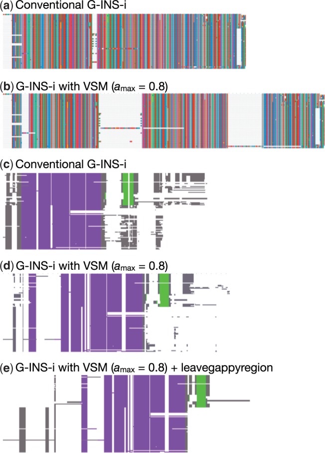
(a) and (b), MSAs of CDK1 sequences with and without VSM, visualized on Jalview (Waterhouse et al., 2009); (c–e), NYN domain (purple), ZF domain (green) and regions without a predicted structure (gray) in MSAs of the zc3h12a-like and N4BP1-like families, with and without VSM. In e, an additional option (- - leavegappyregion; see Supplemental data for details) was applied that tends to return easy-to-understand alignments in gappy regions

The second example illustrates the difficulty of aligning structured protein domains surrounded by intrinsically disordered regions, using two NYN domain-containing protein families (zc3h12a-like and N4BP1-like) as a test case. Both families contain an NYN domain as well as a significant fraction of intrinsically disordered residues; however, the zc3h12a-like family, but not the N4BP1-like family, also contains a C3H zinc finger (ZF) (Marco and Marin, 2009). Figure 2c shows that conventional MAFFT aligns the ZF in the zc3h12a-like family with intrinsically disordered regions in N4BP1. This alignment can cause misidentification of domains or other problems in downstream analyses, without knowledge-based inspection. In contrast, by using VSM (Fig. 2d and e), the ZF domains are automatically separated from intrinsically disordered regions.

3.2 Benchmarks

We conducted benchmark tests based on real and simulated protein sequences to assess the effect of the VSM on accuracy and to determine an appropriate range for the parameter $a_{\text{max}}$. To isolate the effect of the VSM, the G-INS-i option of MAFFT with and without VSM were compared. Actual commands are:

$$\begin{array}{cc}\mathrm{mafft-ginsi}& (\text{G-INS-i\hspace{0.17em}default})\\ \mathrm{mafft-ginsi}\mathrm{--allowshift}\mathrm{--unalignlevel}{a}_{\text{max}}& (\text{G-INS-i\hspace{0.17em}with\hspace{0.17em}VSM})\end{array}$$

Some popular aligners, MUSCLE (Edgar, 2004a, b) v3.8.31, PRANK (with the -F option) (Löytynoja and Goldman, 2008) v150803, MSAprobs (Liu et al., 2010) v0.9.7 and BAli-Phy (Redelings, 2014) v2.3.5 (assuming the WAG (Whelan and Goldman, 2001) + discrete gamma (Yang, 1994) model) were included in the comparison. Since BAli-Phy is not for large datasets, it was applied only to a subset of the benchmark cases with a relatively small number of sequences ($\le 100$). Even in these cases, it was difficult to run BAli-Phy to convergence in a practical amount of time. Therefore, we stopped the calculation at the 1000th cycle. In order not to offset the effect of stopping BAli-Phy before convergence, we ran the program two times from entirely different initial states (unaligned sequences and G-INS-i + VSM alignment) for each problem and included results from both runs in this report. In addition, a simple progressive method, MAFFT-FFT-NS-2, and MAFFT-G-INS-i with the - - leavegappyregion option (used in Fig. 2e) were included in the comparison as reference.

The results of two different protein-based benchmarks, PREFAB (Edgar, 2004b) and OXBench (Raghava et al., 2003), are shown in Figure 3. These datasets are based on protein structural alignments. In relatively difficult cases, only short conserved regions (usually functional sites under strong evolutionary constraint) are aligned in the reference and it is assessed how correctly these sites are aligned by methods to be tested. By using VSM, this type of benchmark score decreased. The amount of decrease depends on the parameter $a_{\text{max}}$; small as $a_{\text{max}}$ approaches 0.8 and relatively large when $a_{\text{max}}=0.9$. The benchmark scores of PRANK and BAli-Phy are low, consistent with a previous study (Sievers et al., 2011). This test does not take the over-alignment problem into account.

Fig. 3.

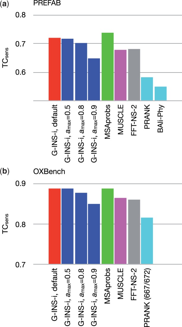
Comparison of sensitivity based on two real protein-based benchmarks. (a) In the PREFAB test, the ${\text{TC}}_{\text{sens}}$ score (Eq. 7) was computed with the qscore program (Edgar, 2004a) and averaged for the 1682 entries. The scores of BAli-Phy with the two initial states were similar to each other, 0.5465 and 0.5480. (b) In the ‘extended’ subset of OXBench, the column score was computed using the run_metric.pl program (Raghava et al., 2003) and averaged for the 672 entries. For PRANK, the average for 667 entries are shown because it failed in five entries. BAli-Phy was not applicable to this test, because the maximum number of sequences in an MSA is 668

It is necessary to simultaneously assess MSA methods with two different criteria: (i) How accurately are functionally or structurally similar regions detected? (ii) How many evolutionarily unrelated sites are correctly gapped (i.e. not over-aligned)? Protein structure-based benchmarks can be used only for (i) as explained in Introduction. As an alternate approach, we used artificial sequences generated under conditions to mimic real protein-based benchmarks; two ‘functional’ regions or catalytic centers, where no insertions/deletions (indels) were allowed, were set in each alignment. Indels were allowed in the remaining regions. Using these artificial sequences, we assessed two different types of alignment quality.

First, sensitivity was assessed using

$${\text{TC}}_{\text{sens}}=\frac{\text{The\hspace{0.17em}number\hspace{0.17em}of\hspace{0.17em}correctly\hspace{0.17em}aligned\hspace{0.17em}columns}}{\text{The\hspace{0.17em}number\hspace{0.17em}of\hspace{0.17em}aligned\hspace{0.17em}columns\hspace{0.17em}in\hspace{0.17em}the\hspace{0.17em}reference}},$$ (7)

where the reference is the alignment of the ‘functional’ regions. There are no gaps in these regions in the simulation setting here. This is an established criterion used in Figure 3 and many benchmark studies based on real data.

Second, we used three different criteria in which the over-alignment problem is taken into account. (i):

$${\text{TC}}_{\text{gap}}=\frac{\text{The\hspace{0.17em}number\hspace{0.17em}of\hspace{0.17em}correctly\hspace{0.17em}aligned\hspace{0.17em}or\hspace{0.17em}gapped\hspace{0.17em}columns}}{\text{The\hspace{0.17em}true\hspace{0.17em}alignment\hspace{0.17em}length}}$$ (8)

was calculated for the regions excluding the ‘functional’ regions. If a column with the same set of residue(s) and the same gap pattern in the reference MSA and the estimated MSA is found, the column is regarded to be correct. We also calculated (ii) a distance $d_{\text{evol}}$ to the true MSA, using the MetAl program (Blackburne and Whelan, 2012b). This metric compares the homology sets (see Blackburne and Whelan, 2012b for the definition) of two MSAs, considering the positional and phylogenetic information about where indel events occurr, where we assumed the true tree topology. In addition, we calculated (iii) the false positive (FP) error rate to assess how correctly unrelated sites are gapped, using the FastSP program (Mirarab and Warnow, 2011). FP means the number of pairs that are aligned in an estimated MSA but not aligned in the true MSA. These three criteria can be calculated only when we know the true positions of the all gaps.

We used INDEliBLE version 1.03 (Fletcher and Yang, 2009) with the WAG model (Whelan and Goldman, 2001) for this simulation. Each artificial sequence was divided into five regions with lengths of 90, 10, 90, 10, 100 in the initial state. The second and fourth regions were set as ‘functional’ regions, where no indels were allowed. Sequences were generated based on a common tree topology, but branch lengths differ between two classes, the ‘functional’ regions and the remaining regions, in order to avoid oversimplification to some extent. In each class, the summation of branch lengths from the root to each terminal node is not constant. To cover various cases from easy ones to difficult ones, we tried all possible eight combinations of the indel rate in non-‘functional’ regions (0.1 and 0.01), maximum distance (0.5 and 2.0) and the number of sequences (100 and 500). The actual setting file is given in Supplemental data. The simulation was repeated 100 times for each of the eight conditions.

The results of this simulation-based benchmark are shown in Figure 4. The vertical axis (${\text{TC}}_{\text{sens}}$) is the standard criterion for alignment accuracy, while the horizontal axis considers over-alignment. The upper eight panels (a–h) and the lower eight panels (a′–h′) use ${\text{TC}}_{\text{gap}}$ and $d_{\text{evol}}$, respectively. Panels e and e′ correspond to a difficult condition (larger dataset with higher indel rate and divergence), while panels d and d′ correspond to an easy condition (smaller dataset with lower indel rate and divergence). A similar comparison using the FP error rate as the horizontal axis is shown in Figure S1.

Fig. 4.

Results of simulation-based benchmark with eight settings. In each panel, the vertical axis is ${\text{TC}}_{\text{sens}}$ (Eq. 7) for aligning the ‘functional’ regions. The horizontal axes of a–h and a$\prime$–h$\prime$ are ${\text{TC}}_{\text{gap}}$ (Eq. 8) and $d_{\text{evol}}$ (Blackburne and Whelan, 2012b), respectively, in which over-alignment is taken into account. Average score and standard deviation for 100 replications for each setting/method/criterion are plotted. Average scores of G-INS-i with $a_{\text{max}}$ values of 0.0–0.9 are plotted as a blue curve in each panel. In e and e$\prime$, PRANK and MUSCLE failed to complete the calculation for 16 and 4 out of the 100 replications, respectively. In g and g$\prime$, PRANK failed for 16 replications. In these cases, the average and standard deviation of the successful runs of each method are shown. BAli-Phy was applied only to the settings with 100 sequences (a–d and a$\prime$–d$\prime$). Results from two different initial states (see main text) are separately shown (upward triangles in cyan), but their difference was negligible

In Figures 4 and S1, the effect of VSM corresponds to the difference between the red filled circle (conventional G-INS-i) and the blue filled square (G-INS-i with VSM). The ${\text{TC}}_{\text{gap}}$ score (horizontal axis of Fig. 4a–h) consistently increased (shifts right on the plot) with the introduction of VSM, in all cases except for the very easy one. Similarly, the distance $d_{\text{evol}}$ and the FP error rate decreased with VSM (Fig. 4a′–h′ and Fig. S1). For the ${\text{TC}}_{\text{sens}}$ score (vertical axis; sensitivity in aligning ‘functional’ regions), the effect of VSM was mostly neutral, but there were even some cases (Fig. 4a and e) where the ${\text{TC}}_{\text{sens}}$ score increased by VSM. When the parameter $a_{\text{max}}$ was 0.9, the benchmark scores became worse in some cases (Fig. 4c and g).

The ${\text{TC}}_{\text{gap}}$ scores of PRANK and BAli-Phy (shown cyan in Fig. 4a–h) were always higher than other methods, while their ${\text{TC}}_{\text{sens}}$ scores were relatively lower for diverged sequences (a, e and g) and for large datasets (e and g). In the $d_{\text{evol}}$ metric (Fig. 4a′–h′), the advantage of PRANK was unclear for large input data (e′–h′). These observations are consistent with the fact that these methods were designed for aligning a small number of closely-related sequences.

Comparing Figures 3 and 4, the sensitivity (measured by ${\text{TC}}_{\text{sens}}$) of PRANK and BAli-Phy was observed to be relatively higher (e.g, relative to MUSCLE) in Figure 4 (simulation) than in Figure 3 (real data). Thus the discrepancy from real benchmarks remains even in this simulation setting. Possibly the evolutionary model was still unrealistically simple. Stronger violation of assumptions might be necessary to reproduce a realistic situation. Moreover, this simulation setting does not explicitly assume the type of alignment used for Figure 1 (adjacent non-homologous regions). Thus there is an inconsistency between the assumption of the proposed method and the evaluation shown in Figure 4. More realistic simulation designs might help a better understanding of the behavior of this method.

The - - leavegappyregion option of MAFFT was used as default previously (till 2013 Oct, versions <7.113). Because this option has a problem in handling a large number of sequences, the default setting was changed since version 7.113 (See Supplemental data for details). Still, the previous default is selectable, with the flag - - leavegappyregion, in the current version, because it returns an easily-understandable MSA for a small number of sequences, as exemplified in Figure 2 e. This is sometimes useful for visual inspection. In Figure 4, the effect of VSM was observed with the - - leavegappyregion option in relatively easy cases (compare red open circles and blue open squares in a, a$\prime$, b and b$\prime$) largely as well as the current default (red filled circles and blue filled squares). When this option was applied to relatively difficult problems with 500 sequences (e, e$\prime$, f$\prime$ and f), the alignment quality in terms of ${\text{TC}}_{\text{gap}}$ and $d_{\text{evol}}$ (horizontal axis) was worse and VSM was less effective than in the current default.

The CPU time for each method to perform the tests is listed in Table 1. By introducing VSM to MAFFT-G-INS-i, the CPU time became several times longer than the normal calculation. The causes of slowdown are digitalization of distance in the iterative refinement step and the increase of alignment length. Since the iterative refinement method is not applicable to a large MSA consisting of thousands of sequences, we are developing a combination of fast progressive method and iterative refinement method for large MSAs (manuscript in preparation).

Table 1.

CPU time for calculating each benchmark dataset

	PREFAB	OXBench	Simulation100	Simulation500
G-INS-i default	53 min	1.8 h	4.3 h	10 days
G-INS-i $a_{\text{max}}=0.8$	3.2 h	6.6 h	12 h	22 days
MSAprobs	12 h	18 h	19 h	26 days
MUSCLE	24 min	22 min	2.1 h	2.4 days
FFT-NS-2	3.1 min	1.5 min	3.1 min	22 min
PRANK	1.8 days	1.4 days	3.8 days	23 days

Each program ran on AMD Opteron(tm) Processor 2344 using a single core. Simulation100 indicates the total CPU time for computing 400 MSAs each with 100 sequences (Fig. 4a–d), and Simulation500 indicates the total CPU time for computing 400 MSAs each with 500 sequences (Fig. 4e–h). BAli-Phy was excluded from this table because we stopped the calculation at the 1000th cycle before convergence. It took several months of CPU time, using different computer systems, for PREFAB and for simulation100.

The proposed method was designed for protein data, but the same calculation is possible for DNA data. We are planning to test its efficacy using real DNA data with ultramicro inversions (Hara and Imanishi, 2011), in which unrelated (must-be-gapped) sites can be unambiguously determined.

4 Discussion

According to Blackburne and Whelan (2012a), MSA methods can be classified into two types, similarity-based ones and evolution-based ones. Similarity-based methods, including MAFFT, have two advantages, speed and applicability to datasets of weaker similarity. However, similarity-based methods tend to be affected by over-alignment, while this tendency is smaller in evolution-based methods, such as PRANK and BAli-Phy. In real protein-based benchmarks and simulation-based benchmarks, we reproduced this difference in tendency between the two types of aligners. The proposed method, VSM, tries to avoid over-alignment while still using similarity information.

By introducing VSM to MAFFT-G-INS-i, the number of correctly gapped sites increased without seriously decreasing correctly aligned sites. In the simulation-based benchmarks, the ${\text{TC}}_{\text{gap}},d_{\text{evol}}$ and FP scores were improved by VSM, but still worse than those of evolution-based methods. On the other hand, the advantage of similarity-based methods over evolution-based methods in sensitivity was kept even with VSM.

This method has an additional parameter, $a_{\text{max}}$. Our results suggest that the side effect of VSM (overlooking conserved regions) is relatively small when $a_{\text{max}}$ is less than or close to 0.8 and drastically increases when $a_{\text{max}}=0.9$. The same tendency was consistently observed in real data (Fig. 3) and simulation (Fig. 4c and g). Therefore $a_{\text{max}}=0.8$ may be a rational setting. A fine tuning of this parameter may be possible but not easy, because there can be more heterogeneous sources of noise than the simulations we tried, in actual data as discussed in Introduction. Here we observed only a general tendency in simple cases. We are planning more realistic benchmarks for specific purposes and/or specific data, such as detection of positively selected sites, phylogenetic inference and NGS data.

4.1 Assumptions and limitations

Generally, the inclusion of entirely non-homologous sequences in an MSA results in unnecessarily long and/or meaningless alignments, and it has to be avoided. In the proposed method, if non-homologous sequences are given, their distances to other sequences are estimated to be large and thus they are normally aligned with a = 0. At present, MAFFT has no function to exclude such divergent input sequences. The proposed method also has other limitations common to conventional MSA methods; the order of letters in each input sequence is completely preserved in the alignment process. Accordingly, domain rearrangement in protein sequences is not considered.

4.2 Perspectives

When gapped regions are not of interest, the over-alignment problem does not need to be considered explicitly. We can apply highly sensitive (and careless about over-alignment) aligners, such as MAFFT-G-INS-i or MSAprobs, followed by filtering methods (Capella-Gutierrez et al., 2009; Castresana, 2000; Chang et al., 2014; Penn et al., 2010). In such an approach, the ability of filtering methods to correctly exclude non-homologous sites is crucial to overall performance. From a practical viewpoint, it is yet unclear which strategy will work best: (i) over-aligned data plus filtering, (ii) less over-aligned data plus filtering, or (iii) less over-aligned data without filtering. The optimal approach will probably depend on multiple factors, including similarity of homologous sequences, data size and purpose of downstream analyses. Careful tests, preferably based on real data, will be necessary.

Possible extensions of the VSM technique include: (i) Use of a more complex function for a(d), such as a sigmoidal dependence. (ii) Use of multiple variable matrices (MVSM), which is a combination of MSM and VSM. It might improve simulation-based benchmark scores further, but Figure 1 suggests that the effect of VSM is dominant in avoiding over-alignment. (iii) BLOSUM and JTT do not completely satisfy the requirements for aligning a mixture of distantly-related sequences and closely-related sequences as discussed in Section 3. This report proposes BLOSUM-VSM as a possible solution. For a better solution, we have a plan to build and use a new series of empirical matrices, each of which is for a strictly specific range of similarity levels, based on MIQS (Yamada and Tomii, 2014). By excluding too remote pairs (unlike BLOSUM), MIQS-VSM, -MSM or -MVSM might result in a better tradeoff between sensitivity and over-alignment. (iv) There is a natural requirement that a stronger gap cost should be applied for closely-related sequences. The proposed method was designed for an apparently opposite requirement; additional gaps should be inserted for a set of highly similar sequences when they have unexpectedly dissimilar segments. Actually, the relationship between the parameter a and gap cost is not simple. The increase of a introduces additional gaps by design, but it functions to replace a number of short gaps with a small number of long gaps, like a strong gap open cost does, as in Figure 1. It may be possible to vary gap cost, too, based on an evolutionary model of indels (eg., Knudsen and Miyamoto, 2003; Redelings and Suchard, 2007). Still, it will be useful to take into account that unexpectedly dissimilar segments can result from non-evolutionary processes such as sequencing errors and mistranslations, in addition to evolutionary process.

Possible applications include: (i) Increasing the diversity of MSAs to quantify residue-wise reliability in perturbation-based methods, such as HoT (Landan and Graur, 2007) or GUIDANCE (Penn et al., 2010). (ii) Providing partial MSAs for integrative aligners, such as MCoffee (Wallace et al., 2006) and PASTA (Mirarab et al., 2015). When more diverged MSAs are necessary, varying a, instead of simply defining $a_{\text{max}}$, may be effective.

In addition to its practical utility, we emphasize the simplicity and extendability of VSM. It is based on natural biological reasoning—different parameters should be used for close and remote homologs in alignment calculations. Therefore, it is compatible with most DP-based MSA calculations. It has just one additional parameter and its meaning is clear, as described in Methods. We speculate that this idea can be used in other MSA methods. For example, the performance of MSAprobs, an HMM-based method, is high in ${\text{TC}}_{\text{sens}}$ but low in ${\text{TC}}_{\text{gap}}$ (Fig. 4). That is, this method is highly sensitive but highly susceptible by over-alignment. ProbCons (Do et al., 2005), an early HMM-based aligner, also has a similar tendency. These methods perform all-to-all pairHMM calculations to obtain probabilistic consistency and then build an MSA progressively using DP matrices derived from the probabilistic consistency. If a VSM-like modification is made on the DP matrices in the second step, it may suppress over-alignment of these methods.

In the field of similarity search, Mills and Pearson (2013) recently proposed to realign query and target with an appropriate scoring matrix according to the similarity level, to give more accurate alignment boundaries avoiding ‘over extension’. They addressed single-to-single local alignment, but the over extension problem can occur when the profile of an MSA is used as a query, too. We expect the proposed method can contribute to the improvement in query MSA construction. That is, there is a possibility that an ‘over-aligned’ query MSA by conventional methods could have a negative effect (possibly over extension) on the similarity search step. By avoiding over-alignment without missing functional or structurally conserved regions in the query MSA, better results may be realized in similarity searches, but this should also be tested on actual data in the future.

Funding

This research is supported by the Platform Project for Supporting in Drug Discovery and Life Science Research (Platform for Drug Discovery, Informatics, and Structural Life Science) from Japan Agency for Medical Research and Development (AMED).

Conflict of Interest: none declared.

References

- Barton G.J., Sternberg M.J. (1987) A strategy for the rapid multiple alignment of protein sequences. confidence levels from tertiary structure comparisons. J. Mol. Biol., 198, 327–337. [DOI] [PubMed] [Google Scholar]
- Berger M.P., Munson P.J. (1991) A novel randomized iterative strategy for aligning multiple protein sequences. Comput. Appl. Biosci., 7, 479–484. [DOI] [PubMed] [Google Scholar]
- Blackburne B.P., Whelan S. (2012a) Class of multiple sequence alignment algorithm affects genomic analysis. Mol. Biol. Evol., 30, 642–653. [DOI] [PubMed] [Google Scholar]
- Blackburne B.P., Whelan S. (2012b) Measuring the distance between multiple sequence alignments. Bioinformatics, 28, 495–502. [DOI] [PubMed] [Google Scholar]
- Bradley R.K. et al. (2009) Fast statistical alignment. PLoS Comput. Biol., 5, e1000392.. [DOI] [PMC free article] [PubMed] [Google Scholar]
- Brent M.R. (2005) Genome annotation past, present, and future: how to define an ORF at each locus. Genome Res., 15, 1777–1786. [DOI] [PubMed] [Google Scholar]
- Capella-Gutierrez S. et al. (2009) trimAl: a tool for automated alignment trimming in large-scale phylogenetic analyses. Bioinformatics, 25, 1972–1973. [DOI] [PMC free article] [PubMed] [Google Scholar]
- Castresana J. (2000) Selection of conserved blocks from multiple alignments for their use in phylogenetic analysis. Mol. Biol. Evol., 17, 540–552. [DOI] [PubMed] [Google Scholar]
- Chang J.M. et al. (2014) TCS: a new multiple sequence alignment reliability measure to estimate alignment accuracy and improve phylogenetic tree reconstruction. Mol. Biol. Evol., 31, 1625–1637. [DOI] [PubMed] [Google Scholar]
- Dayhoff M.O. et al. (1978). A model of evolutionary change in proteins In: Dayhoff M.O., Ech R.V. (eds) Atlas of Protein Sequence and Structure. National Biomedical Research Foundation, Washington, DC, pp. 345–352. [Google Scholar]
- Do C.B. et al. (2005) ProbCons: Probabilistic consistency-based multiple sequence alignment. Genome Res., 15, 330–340. [DOI] [PMC free article] [PubMed] [Google Scholar]
- Edgar R.C. (2004a) MUSCLE: a multiple sequence alignment method with reduced time and space complexity. BMC Bioinf., 5, 113.. [DOI] [PMC free article] [PubMed] [Google Scholar]
- Edgar R.C. (2004b) MUSCLE: multiple sequence alignment with high accuracy and high throughput. Nucleic Acids Res., 32, 1792–1797. [DOI] [PMC free article] [PubMed] [Google Scholar]
- Edgar R.C. (2010) Quality measures for protein alignment benchmarks. Nucleic Acids Res., 38, 2145–2153. [DOI] [PMC free article] [PubMed] [Google Scholar]
- Feng D.F., Doolittle R.F. (1987) Progressive sequence alignment as a prerequisite to correct phylogenetic trees. J. Mol. Evol., 25, 351–360. [DOI] [PubMed] [Google Scholar]
- Fletcher W., Yang Z. (2009) INDELible: a flexible simulator of biological sequence evolution. Mol. Biol. Evol., 26, 1879–1888. [DOI] [PMC free article] [PubMed] [Google Scholar]
- Gonnet G.H. et al. (1992) Exhaustive matching of the entire protein sequence database. Science, 256, 1443–1445. [DOI] [PubMed] [Google Scholar]
- Gotoh O. (1996) Significant improvement in accuracy of multiple protein sequence alignments by iterative refinement as assessed by reference to structural alignments. J. Mol. Biol., 264, 823–838. [DOI] [PubMed] [Google Scholar]
- Gotoh O. et al. (2014) Assessment and refinement of eukaryotic gene structure prediction with gene-structure-aware multiple protein sequence alignment. BMC Bioinf., 15, 189.. [DOI] [PMC free article] [PubMed] [Google Scholar]
- Hara Y., Imanishi T. (2011) Abundance of ultramicro inversions within local alignments between human and chimpanzee genomes. BMC Evol. Biol., 11, 308.. [DOI] [PMC free article] [PubMed] [Google Scholar]
- Henikoff S., Henikoff J.G. (1992) Amino acid substitution matrices from protein blocks. Proc. Natl. Acad. Sci. U. S. A., 89, 10915–10919. [DOI] [PMC free article] [PubMed] [Google Scholar]
- Higgins D.G., Sharp P.M. (1988) CLUSTAL: a package for performing multiple sequence alignment on a microcomputer. Gene, 73, 237–244. [DOI] [PubMed] [Google Scholar]
- Jones D.T. et al. (1992) The rapid generation of mutation data matrices from protein sequences. Comput. Appl. Biosci., 8, 275–282. [DOI] [PubMed] [Google Scholar]
- Katoh K., Standley D.M. (2013) MAFFT multiple sequence alignment software version 7: improvements in performance and usability. Mol. Biol. Evol., 30, 772–780. [DOI] [PMC free article] [PubMed] [Google Scholar]
- Katoh K. et al. (2002) MAFFT: a novel method for rapid multiple sequence alignment based on fast Fourier transform. Nucleic Acids Res., 30, 3059–3066. [DOI] [PMC free article] [PubMed] [Google Scholar]
- Knudsen B., Miyamoto M.M. (2003) Sequence alignments and pair hidden Markov models using evolutionary history. J. Mol. Biol., 333, 453–460. [DOI] [PubMed] [Google Scholar]
- Landan G., Graur D. (2007) Heads or tails: a simple reliability check for multiple sequence alignments. Mol. Biol. Evol., 24, 1380–1383. [DOI] [PubMed] [Google Scholar]
- Liu Y. et al. (2010) MSAProbs: multiple sequence alignment based on pair hidden Markov models and partition function posterior probabilities. Bioinformatics, 26, 1958–1964. [DOI] [PubMed] [Google Scholar]
- Löytynoja A., Goldman N. (2005) An algorithm for progressive multiple alignment of sequences with insertions. Proc. Natl. Acad. Sci. U. S. A., 102, 10557–10562. [DOI] [PMC free article] [PubMed] [Google Scholar]
- Löytynoja A., Goldman N. (2008) Phylogeny-aware gap placement prevents errors in sequence alignment and evolutionary analysis. Science, 320, 1632–1635. [DOI] [PubMed] [Google Scholar]
- Marco A., Marin I. (2009) CGIN1: a retroviral contribution to mammalian genomes. Mol. Biol. Evol., 26, 2167–2170. [DOI] [PubMed] [Google Scholar]
- Mills L.J., Pearson W.R. (2013) Adjusting scoring matrices to correct overextended alignments. Bioinformatics, 29, 3007–3013. [DOI] [PMC free article] [PubMed] [Google Scholar]
- Mirarab S., Warnow T. (2011) FastSP: linear time calculation of alignment accuracy. Bioinformatics, 27, 3250–3258. [DOI] [PubMed] [Google Scholar]
- Mirarab S. et al. (2015) PASTA: ultra-large multiple sequence alignment for nucleotide and amino-acid sequences. J. Comput. Biol., 22, 377–386. [DOI] [PMC free article] [PubMed] [Google Scholar]
- Nagy A., Patthy L. (2013) MisPred: a resource for identification of erroneous protein sequences in public databases. Database, 2013, doi:10.1093/database/bat053.. [DOI] [PMC free article] [PubMed] [Google Scholar]
- Needleman S.B., Wunsch C.D. (1970) A general method applicable to the search for similarities in the amino acid sequence of two proteins. J. Mol. Biol., 48, 443–453. [DOI] [PubMed] [Google Scholar]
- Notredame C. et al. (1998) COFFEE: an objective function for multiple sequence alignments. Bioinformatics, 14, 407–422. [DOI] [PubMed] [Google Scholar]
- Penn O. et al. (2010) An alignment confidence score capturing robustness to guide tree uncertainty. Mol. Biol. Evol., 27, 1759–1767. [DOI] [PMC free article] [PubMed] [Google Scholar]
- Raghava G.P. et al. (2003) OXBench: a benchmark for evaluation of protein multiple sequence alignment accuracy. BMC Bioinf., 4, 47.. [DOI] [PMC free article] [PubMed] [Google Scholar]
- Redelings B. (2014) Erasing errors due to alignment ambiguity when estimating positive selection. Mol. Biol. Evol., 31, 1979–1993. [DOI] [PMC free article] [PubMed] [Google Scholar]
- Redelings B.D., Suchard M.A. (2007) Incorporating indel information into phylogeny estimation for rapidly emerging pathogens. BMC Evol. Biol., 7, 40.. [DOI] [PMC free article] [PubMed] [Google Scholar]
- Schwartz A.S., Pachter L. (2007) Multiple alignment by sequence annealing. Bioinformatics, 23, e24–e29. [DOI] [PubMed] [Google Scholar]
- Sievers F. et al. (2011) Fast, scalable generation of high-quality protein multiple sequence alignments using Clustal Omega. Mol. Syst. Biol., 7, 539.. [DOI] [PMC free article] [PubMed] [Google Scholar]
- Suchard M.A., Redelings B.D. (2006) BAli-Phy: simultaneous Bayesian inference of alignment and phylogeny. Bioinformatics, 22, 2047–2048. [DOI] [PubMed] [Google Scholar]
- Thompson J.D. et al. (1994) CLUSTAL W: improving the sensitivity of progressive multiple sequence alignment through sequence weighting, position-specific gap penalties and weight matrix choice. Nucleic Acids Res., 22, 4673–4680. [DOI] [PMC free article] [PubMed] [Google Scholar]
- Thompson J.D. et al. (2011) A comprehensive benchmark study of multiple sequence alignment methods: current challenges and future perspectives. PLoS One, 6, e18093.. [DOI] [PMC free article] [PubMed] [Google Scholar]
- Vingron M., Waterman M.S. (1994) Sequence alignment and penalty choice. review of concepts, case studies and implications. J. Mol. Biol., 235, 1–12. [DOI] [PubMed] [Google Scholar]
- Wallace I.M. et al. (2006) M-Coffee: combining multiple sequence alignment methods with T-Coffee. Nucleic Acids Res., 34, 1692–1699. [DOI] [PMC free article] [PubMed] [Google Scholar]
- Waterhouse A.M. et al. (2009) Jalview Version 2 – a multiple sequence alignment editor and analysis workbench. Bioinformatics, 25, 1189–1191. [DOI] [PMC free article] [PubMed] [Google Scholar]
- Whelan S., Goldman N. (2001) A general empirical model of protein evolution derived from multiple protein families using a maximum-likelihood approach. Mol. Biol. Evol., 18, 691–699. [DOI] [PubMed] [Google Scholar]
- Yamada K., Tomii K. (2014) Revisiting amino acid substitution matrices for identifying distantly related proteins. Bioinformatics, 30, 317–325. [DOI] [PMC free article] [PubMed] [Google Scholar]
- Yandell M., Ence D. (2012) A beginner’s guide to eukaryotic genome annotation. Nat. Rev. Genet., 13, 329–342. [DOI] [PubMed] [Google Scholar]
- Yang Z. (1994) Maximum likelihood phylogenetic estimation from DNA sequences with variable rates over sites: approximate methods. J. Mol. Evol., 39, 306–314. [DOI] [PubMed] [Google Scholar]
Associated Data
This section collects any data citations, data availability statements, or supplementary materials included in this article.