Exploring Automatic Prostate Histopathology Image Gleason Grading via Local Structure Modeling

Abstract

Gleason-grading of prostate cancer pathology specimens reveal the malignancy of the cancer tissues, thus provides critical guidance for prostate cancer diagnoses and treatment. Computer-aided automatic grading methods have been providing efficient and result-consistent alternative to traditional manually slide reading approach, through statistical and structural feature analysis of the digitized pathology slides. In this paper, we propose a novel automatic Gleason grading algorithm through local structure model learning and classification. We use attributed graph to represent the tissue glandular structures in histopathology images; representative sub-graphs features were learned as bags-of-words features from labeled samples of each grades. Then structural similarity between sub-graphs in the unlabeled images and the representative sub-graphs were obtained using the learned codebook. Gleason grade was given based on an overall similarity score. We validated the proposed algorithm on 300 prostate histopathology images from the TCGA dataset, and the algorithm achieved average grading accuracy of 91.25%, 76.36% and 64.75% on images with Gleason grade 3, 4 and 5 respectively.

I. Introduction

Prostate cancer has become the 2nd most common cancer in American men, and also the 2nd leading cause of cancer death in American men, according to the latest statistics from the American Cancer Society reported in March, 2014 [1]. Successful treatment for prostate cancer largely depends on early diagnosis [20], which is determined mainly via the pathology analysis of biopsy samples [2].

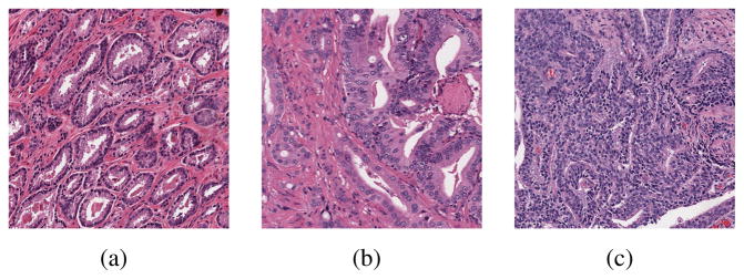
As there are major biological deformation to the tissue cell structure as prostate cancer originates and develops, a grading system based on tissue cells deformation, the Gleason grading system [3], was developed and widely adopted to measure the malignance of caner tissue. In the Gleason system, a grade of 1 to 5 is given to the sampled prostate tissue based on the tissue architecture. Grade 1 corresponds to well-differentiated structure with the highest degree of resemblance to normal tissues, while grade 5 corresponds to poorly differentiated tissue with the highest degree of resemblance to cancer tissues. In pathology practice, only tissue with a Grade of 3 and higher are considered carcinoma, so in this work we only focus on the inter-class classification among Grade 3, 4, and 5. Figure 1 illustrated the representative tissue samples of Gleason score 3, 4 and 5.

Fig. 1.

Example histopathology images of Gleason grade 3(a), grade 4(b) and grade 5(c).

With the widely used of digital pathology systems and whole-slide imaging (WSI) technology in prostate cancer research field, lots of work has been dedicated in developing automatic analysis and grading algorithms [4]–[10] in the past few years. Early auto-grading algorithm [4], [5] used statistical features to capture the structure differences between tissue images of different grades. Huang et.al [4] used fractal-dimension (FR), a texture feature to capture the local-repentance appeared in tissue patches. Doyle et al. [5] combined first-order statistic feature with texture features (co-occurrence feature [11] and Gabor feature [12]), and generated a concatenated feature of 927 dimensions. Although showed good classification accuracies, it requires a higher feature dimension to achieve high classification accuracy, as well as effective feature selection and dimension reduction methods. In work [5], Doyle et al. used AdaBoost [13] classifier to select the most effective features from the 927 dimension feature.

Later research [6]–[10] tried to directly extract the component-level information from the tissue images by modeling and quantifying the organization and distribution of the histopathological components within tissues. In work [6]–[9], graph-based feature were proposed to model and quantify global structural organization. Recently, Ozdemir et al. [10] introduced to use attributed sub-graph to model the local structural features. However in the work, the classifications were conducted in a semi-automatic way through comparing to pre-selected sub-graphs from groud-truth query images.

Inspired by the work in [10] in this paper we propose a novel automatic Gleason grading algorithm based on local structural modeling. We use attributed graph to represent the tissue glandular structures in histopathology images, and introduce a distribution histogram to model the labeled subgraph and quantify the similarity between local structures. The rest of the paper is organized as follows, in Section II we describe our local structure feature modeling based automatic-grading algorithm; the evaluation results were detailed in Section III; with concluding remarks in Section IV.

II. Methodology

A. Overview

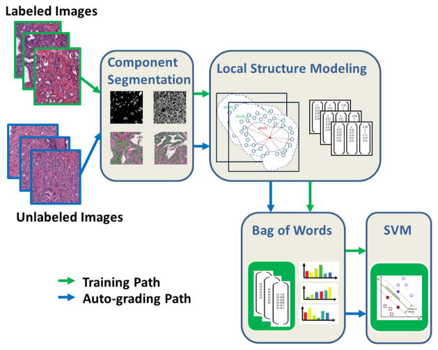
Figure 2 gives an overview of the proposed automatic grading method. The method is composed of 2 phases: training phase and auto-grading phase. (1) During the training phase, sub-graphs were built based on the segmented tissue components (nuclei and lumen in this study), and the local structure features were extracted from the sub-graphs. A codebook was learned from the local structure feature set using bag-of-words [15] method. Then based on the learned codebook, each set of local structure features can be represented using one word-frequency feature. A multi-class SVM classifier was then trained from the word-frequency features. (2) During the auto-grading phase, local structure features were extracted similarly from the sub-graphs built on the unlabeled input image, and the class label of the unlabeled image were assigned by the multi-class SVM classifier using the word-frequency features mapped from the codebook. Each step will be detailed in the following sections.

Fig. 2.

Overview of the proposed algorithm.

B. Tissue Component Segmentation

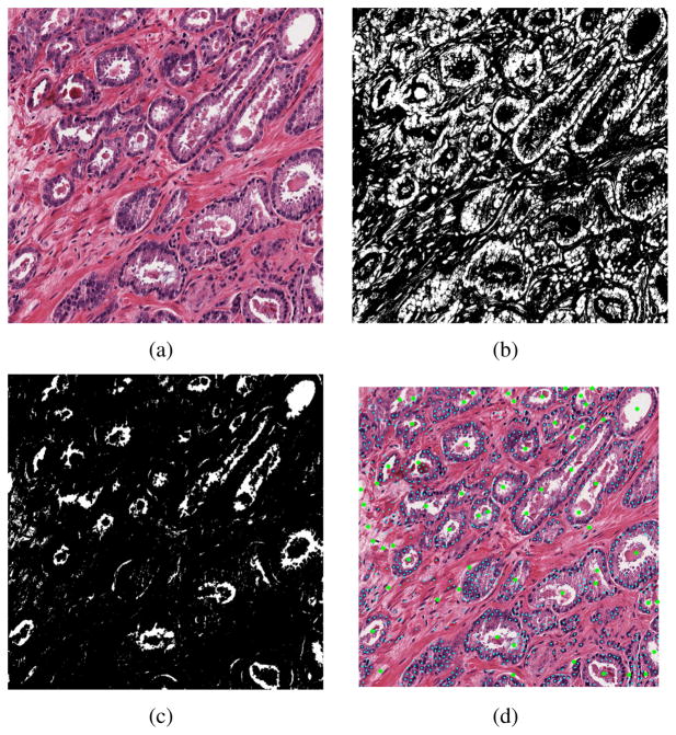
In order to capture the centroids of the lumen regions, we used a 2-level segmentation method. In the 1st level, tissue image were segmented into 4 groups: nuclei, lumen, stroma and cytoplasm using a trained Bayes classifier. The classifier used the RGB value as the feature and trained from a labeled sample set of 1600 points, with 400 points from each category. Then in level-2, we adopted the method from [14] and used Fast Radial Symmetry Transform (FRST) feature as marker to perform a marker-controlled watershed segmentation. The centroids were refined using additional criterias. Figure 3(c) and 3(b) showed the segmented nuclei and lumen region of a sample image (Figure 3(a)), and the nuclei and lumen centroids from level-2 segmentation were showed in Figure 3(d).

Fig. 3.

Lumen and nuclei segmentation. (a) Original image, (b)segmented nuclei region, (c) segmented lumen regions, (d) detected lumen and nuclei centroids.

C. Local Structure Modeling

As illustrated in Figure 1, the spatial distribution and organization of nuclei and lumen in the prostate tissue characterize the malignance of the tissue sample. In this method, we only focus on building a tissue graph to represent the spatial distribution of nuclei and lumen in the tissue sample.

1) Local Structure Grouping

Normal prostate histopathology tissue consists of gland units surrounded by fibromuscular tissue (named stroma), which mechanically supports the gland units. Each gland unit is composed of rows of epithelial cells situated around a duct(named lumen). To better capture the glandular structure in the tissue, we group the tissue component into lumen-centered local groups. Let NucC and LumC represent the centroid sets of the segmented nuclei and lumen region in the image, with N_nuc and N_lum equal the number of nuclei and lumen regions segmented. And define LumB_iL as the iL_th lumen boundary, in which iL ∈ [1, 2, ..., N_lum]. To group the nuclei with its nearest lumen area, we define the grouping criteria as in Equation 1 and Equation 2.

$${\mathit{gid}}_i^N=j,\forall i\in [1,2,\dots ,N_{\mathit{lum}}],{\mathit{Dis}}_j^{\mathit{NLc}}<{\mathit{Dis}}_i^{\mathit{NLc}}$$ (1)

$${\mathit{Dis}}_i^{\mathit{NLc}}=\mathit{min}({\mathit{dis}}_{j,k}^{\mathit{NLb}}),k\in {\text{LumB}}_{jL}$$ (2)

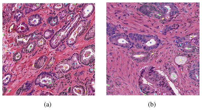
In which, ${\mathit{gid}}_i^N$ is the grouping label of the i_th nuclei, ${\mathit{Dis}}_{j,k}^{\mathit{NLb}}$ represent the distance between the i_th nuclei and the j_th lumen boundary point. Figure 4 showed the grouping results of nuclei and lumen elements on sample images of grade 3 and grade 4.

Fig. 4.

Nuclei-lumen local grouping result of grade 3(a) and grade 4(b) images.

2) Lumen-nuclei Co-location (LNCL) Feature

In this work, we design a new feature lumen-nuclei co-location (LNCL) to quantize the organization and distribution of nuclei and lumen in a local group. LNCL feature is built to model the statistic distribution of distance and tilting angle between each pair of component elements in a local glandular group. In our study, we use 2 groups of component elements: nuclei-lumen (NL) and nuclei-nuclei (NN). Figure 5 illustrate the NL and NN pairs on a pseudo gland unit. LNCL feature is defined as:

$$\mathit{LNCL}=[{\mathit{hist}}_{\mathit{dis}}^{NL},{\mathit{hist}}_{\mathit{ang}}^{NL},{\mathit{hist}}_{\mathit{dis}}^{NN},{\mathit{hist}}_{\mathit{ang}}^{NN}],$$ (3)

Fig. 5.

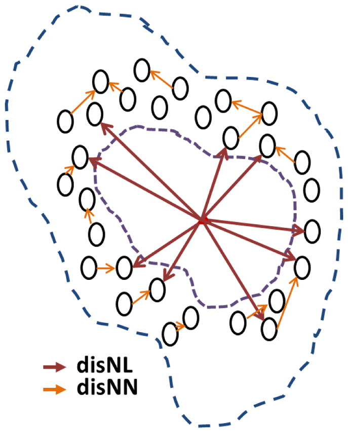
Illustration of LNCL feature on a pseudo gland.

In which, ${\mathit{hist}}_{\mathit{dis}}^{NL}({\mathit{hist}}_{\mathit{dis}}^{NN}),{\mathit{hist}}_{\mathit{ang}}^{NL}({\mathit{hist}}_{\mathit{ang}}^{NN})$ represent the histogram of distance and tilting angle between the nuclei-lumen (nuclei-nuclei) pairs within a local glandular group.

3) Relaxed-LNCL (rLNCL) Feature

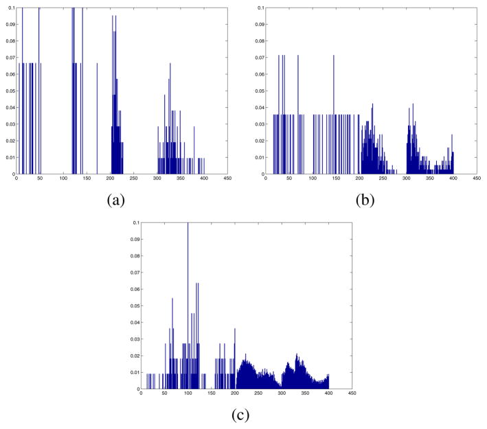
Due to the histopathology structure, lumen regions were not present in some tissue structures. Using the grouping criteria, in these cases, the nuclei will be grouped with the nearest lumen element. Although not grouped as exist glandular unit, the histograms (in Equation 3) still captures the organization and distribution of between the nuclei, we refer to them as relaxed-LNCL features. Figure 6 showed example LNCL (rLNCL) feature from sample structure group from tissue of different Gleason grade.

Fig. 6.

LNCL (rLNCL) feature from sample structure group of Grade 3(a), 4(b) and 5(c) tissue region.

D. Grade Classification through Bags of Words

To quantify the element-wise similarity between structure groups from different images, we adopt the bag-of-words [15] paradigm for LNCL based grade classification. Here we use K-means [16] clustering algorithm and hard-assign to build a codebook from the LNCL (rLNCL) feature set calculated with all labeled (training) images. Then a 3-class SVM classifier (one-vs-one) was trained using the mapped word-frequency feature. With the learned classifier, during the auto-grading phase, the output of the 3-class SVM will be the auto-grading label for the unlabeled input image.

III. Experimental Evaluation

A. Dataset

We tested the proposed auto-grading algorithm on a dataset of 300 H&E stained prostate histopathology images. The images were selected as region-of-interest (ROI)s of whole-slide images from National Cancer Institute (NCI) [18] the Cancer Genome Atlas (TCGA) [19] database. The ROIs were sampled at 40X magnification, and pixel resolution of 2048×2048 from the whole-slide images. The images are chosen evenly with ground-truth labeled Grade 3, 4 and 5.

B. Results

1) Classification Accuracy

We evaluated the grading algorithm using 10-folds cross validation, and the classification accuracy on images of groud-truth Gleason scores 3, 4 and 5 are showed in Table I. Here we use codebook size K = 300.

TABLE I.

Classification Accuracy on Dataset with Different Ground-truth Gleason Score %

Test Dataset	High	Low	Average
Grade 3 carcinoma	93.75	87.50	91.25
Grade 4 carcinoma	86.36	63.64	76.36
Grade 5 carcinoma	72.72	60.81	64.75

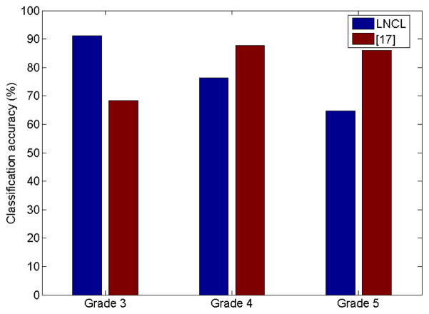
We further evaluate the proposed local-structure based LNCL (rLNCL) feature by comparing it with our statistic feature based former work [17]. Comparison results in Figure 7 showed that structure feature outperformed statistic feature in testing images with more structural characteristic (Grade 3).

Fig. 7.

Classification accuracy comparison between the proposed algorithm and classification algorithm in [17].

2) Parameter Analysis

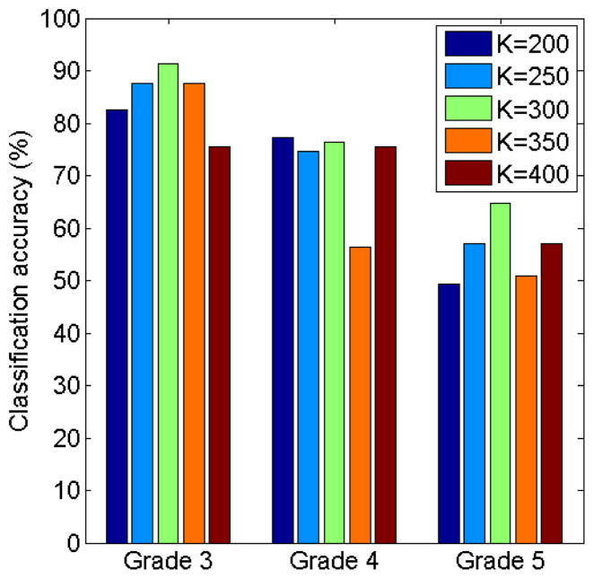
To test the bag-of-words paradigm under different parameters, we evaluated the performance of the classification using different codebook sizes, K ∈ {200, 250, 300, 350, 400}. The classification accuracy of the proposed algorithm under different codebook sizes were showed below in Figure 8.

Fig. 8.

Classification accuracy of the proposed algorithm under different codebook sizes.

IV. Conclusion

In this paper, we proposed a novel automatic Gleason grading algorithm through supervised tissue structure learning and supervised classification. Representative sub-graphs features were modeled by a novel lumen-nuclei co-location (LNCL) feature and learned as bags-of-words features from labeled samples of each grades. Structural similarity between sub-graphs in the unlabeled images and the representative sub-graphs were obtained using the learned codebook and 3-class SVM classifier. Validation on sampled prostate histopathology images showed average grading accuracy of 91.25%, 76.36% and 64.75% respectively on Grade 3, 4 and 5 samples respectively.

References

- 1.American Cancer Society. http://www.cancer.org.
- 2.Matlaga B, Eskew L, McCullough D. Prostate biopsy: Indications and technique. J Urol. 2003;169(1):12–19. doi: 10.1016/S0022-5347(05)64024-4. [DOI] [PubMed] [Google Scholar]
- 3.Gleason D. Classification of prostate carcinomas. Cancer Chemother Rep. 1966;50(3):125–128. [PubMed] [Google Scholar]
- 4.Huang P, Lee C. Automatic classification for pathological prostate images based on fractal analysis. IEEE Transaction on Medical Imaging. 2009 Jul;28(7):1037–1350. doi: 10.1109/TMI.2009.2012704. [DOI] [PubMed] [Google Scholar]
- 5.Doyle S, Feldman M, Tomaszewski J, Madabhushi A. A boosted Bayesian multiresolution classifier for prostate cancer detection from digitized needle biopsies. IEEE Transaction on Biomedical Engineering. 2012 May;59(5):1205–1218. doi: 10.1109/TBME.2010.2053540. [DOI] [PubMed] [Google Scholar]
- 6.Doyle S, Hwang M, Shah K, Madabhushi A, et al. Automated grading of prostate cancer using architectural and textural image features. Biomedical Imaging: From Nano to Macro, 2007. ISBI 2007. 4th IEEE International Symposium on; pp. 1284–1287. [Google Scholar]
- 7.Basavanhally AN, Ganesan S, Agner S, Monaco JP, Feldman MD, Tomaszewski JE, Bhanot G, Madabhushi A. Computerized image-based detection and grading of lymphocytic infiltration in HER2+ breast cancer histopathology. IEEE Transaction on Biomedical Engineering. 2010 Mar;57(3):642–653. doi: 10.1109/TBME.2009.2035305. [DOI] [PubMed] [Google Scholar]
- 8.Jondet M, Agoli-Agbo R, Dehennin L. Automatic measurement of epithelium differentiation and classification of cervical intraneoplasia by computerized image analysis. Diagnostic Pathol. 2010;5(7) doi: 10.1186/1746-1596-5-7. [DOI] [PMC free article] [PubMed] [Google Scholar]
- 9.Altunbay D, Cigir C, Sokmensuer C, Gunduz-Demir C. Color graphs for automated cancerdiagnosis and grading. IEEE Transaction on Biomedical Engineering. 2010 Mar;57(3):665–674. doi: 10.1109/TBME.2009.2033804. [DOI] [PubMed] [Google Scholar]
- 10.Ozdemir E, Grunduz-Demir C. A hybrid classification model for digital pathology using structural and statistical pattern recognition. IEEE Transaction on Medical Imaging. 2013 Feb;32(2):474–483. doi: 10.1109/TMI.2012.2230186. [DOI] [PubMed] [Google Scholar]
- 11.Haralick R, Shanmugam K, Dinstein I. Textural features for image classification. IEEE Trans Syst, Man Cybern. 1973 Nov;SMC-3(6):610–621. [Google Scholar]
- 12.Jain A, Farrokhnia F. Unsupervised texture segmentation using gabor filters. Proc IEEE Int Conf Syst, Man, Cybern. 1990:14–19. [Google Scholar]
- 13.Freund Y, Schapire R. Experiments with a new boosting algorithm. Proc 13th Int Conf Mach Learning. 1996:148–156. [Google Scholar]
- 14.Veta M, van Diest PJ, et al. Automatic nuclei segmentation in H&E stained breast cancer histopathology images. Proc INTERMAG Conf. 1987 doi: 10.1371/journal.pone.0070221. 2.2-12.2-6. [DOI] [PMC free article] [PubMed] [Google Scholar]
- 15.Sivic J, Zisserman A. Video google: A text retrieval approach to object matching in videos. ICCV. 2003 [Google Scholar]
- 16.Lloyd SP. Least squares quantization in PCM. IEEE Transactions on Information Theory. 28(2):129–137. [Google Scholar]
- 17.Wang D, Granados MD, et al. High-throughput automatic Gleason-grading system for prostate histopathology images using CometCloud. The 7th International Workshop on High Performance Computing for Biomedical Image Analysis (HPC-MICCAI); Boston. pp. 21–30. [Google Scholar]
- 18.The National Cancer Institute. http://www.cancer.gov.
- 19.The Cancer Genome Atlas. http://cancergenome.nih.gov.
- 20.Wolf AMD, Wender RC, et al. American Cancer Society Guideline for the Early Detection of Prostate Cancer. American Cancer Society (ACS) 2010 doi: 10.3322/caac.20066. [DOI] [PubMed] [Google Scholar]