On Two Numerical Techniques for Light Scattering by Dielectric Agglomerated Structures

Abstract

Smoke agglomerates are made of many soot sphcres, and their light scattering response is of interest in fire research. The numerical techniques chiefly used for theoretical scattering studies are the method of moments and the coupled dipole moment. The two methods have been obtained in this tutorial paper directly from the monochromatic Maxwell curl equations and shown to be equivalent. The effects of the finite size of the primary spheres have been numerically delineated.

1. Introduction

Electromagnetic scattering problems involving complicated geometries are treated numerically nowadays. Apart from some low- or high-frequency methods [1, 2] and the T-matrix method [3], implementation of most numerical techniques entails a partitioning of the region occupied by the scatterer into may subregions. This is generally true whether a differential formulation is used or an integro differential formalism.

The method of moments (MOM) [4–6], as applied to an inhomogeneous dielectric scatterer, is an approach based on the evaluation of an electric field volume integral equation over the region occupied by the scatterer. This region is partitioned into a number of subregions; the electric field in each subregion is represented by a subregional basis function; and the volume integral equation is converted into a set of simultaneous algebraic equations that are solved using standard procedures. The subregions are generally cubes, although the relevant self-terms are usually evaluated as that of equivoluminal spheres.

Whereas the MOM is an actual field formalism, the coupled dipole method (CDM) is based on the concept of an exciting field. The CDM was formulated intuitively in 1969 by Purcell and Pennypacker [7] for dielectric scatterers, although it had by that time a rich history spanning many decades [8]. Conceived from a microscopic viewpoint, the CDM has only a semi-microscopic basis; indeed, the operational basis for applying the CDM to boundary value problems is totally macroscopic [9]. Both the MOM and the CDM were recently extended to bianisotropic scatterers and their respective weak and strong forms were shown to be equivalent [10].

This tutorial paper contains a complete derivation of the MOM and the CDM for the scattering of time-harmonic electromagnetic waves by an inhomogeneous dielectric object possessing an isotropic permittivity, the starting point of the exercise being the monochromatic Maxwell curl equations. A central topic of the paper is the elucidation of the relationship between the MOM, which is widely used in electrical engineering, and the CDM, which is motivated by concepts in atomic physics [7]. Our treatment is directed towards the researcher who is interested in understanding these methods but who may not be a specialist in electromagnetic field theory.

A current topic of considerable interest is light scattering by agglomerated structures made up of individual spheres arranged in a low-density structure. Examples of such structures include smoke agglomerates formed in fires or internal combustion engines; various materials produced in combustion systems including silica and titanium dioxide; and, perhaps, interstellar dust. The earliest relevant analyses [11, 12] of light scattering from smoke were based on the Rayleigh-Debye approximation, in which the field exciting any particular primary sphere is taken to be just the field that is actually incident on the agglomerate. Such a procedure neglects multiple scattering effects, and is acceptable for primary spheres with size parameter (= radius multiplied by the free space wavenumber) less than about 0.2. The typical size parameters for the smoke agglomerates mentioned above lie in the range 0.1 to about 0.25 at visible frequencies.

Both the CDM [13, 14] and the MOM [15, 16] have been applied to compute scattering from smoke agglomerates in the recent past, since neither technique suffers from the limitations of the Rayleigh-Debye approximation. While the MOM and the CDM are expected to give the same results for infinitesimally small size parameters [17], the methods – as ordinarily used – do not yield identical results as the primary sphere size increases [18, 19]. This is because the CDM has been used chiefly in what may be called its weak form, while it is the strong form of the MOM that is in standard usage [10]. The strong form is valid for larger primary spheres because the effect of the singularity of the free space dyadic Green’s function is better estimated therein than in the weak form. This becomes clearer in the following sections.

2. Volume Integral Equation

As is schematically illustrated in Fig. 1, let all space be divided into two mutually disjoint regions, V_int and V_ext, that are distinguishable from each other by the occupancy of matter. The region V_ext is vacuous; hence,

$$\mathit{D}(\mathit{x})={ϵ}_0\mathit{E}(\mathit{x});\mathit{x}\in V_{\text{ext}.}$$ (1a)

$$\mathbf{B}(\mathit{x})={\mu }_0\mathit{H}(\mathit{x});\mathit{x}\in V_{\text{ext}}.$$ (1b)

Fig. 1.

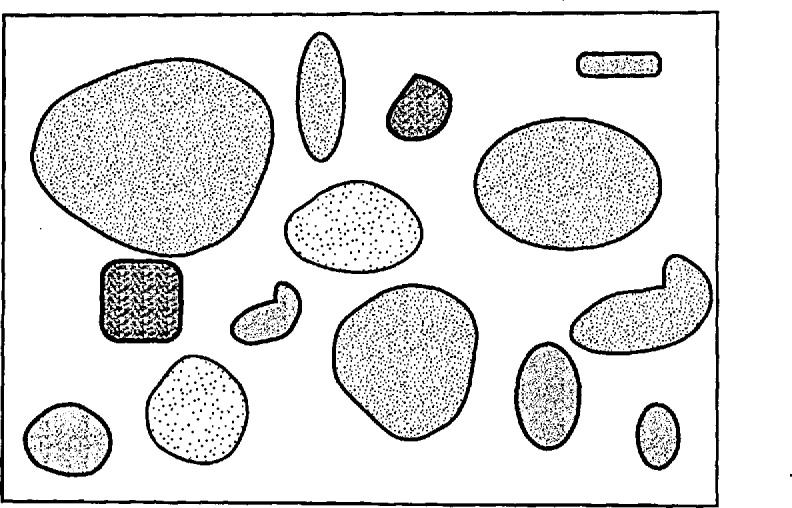
Schematic of the scattering problem. The unshaded region V_ext extends to infinity in all directions, while the shaded regions collectively constitutc V_int.

The region V_int is filled with an isotropic, linear, possibly inhomogeneous, dielectric continuum with frequency dependent [exp(−iωt)] constitutive equations

$$\mathit{D}(\mathit{x})={ϵ}_0{ϵ}_{\mathrm{r}}(\mathit{x})\mathit{E}(\mathit{x});\mathit{x}\in V_{\mathrm{int}},$$ (2a)

$$\mathbf{B}(\mathit{x})={\mu }_0\mathit{H}(\mathit{x});\mathit{x}\in V_{\mathrm{int}},$$ (2b)

where ϵ_r(x) is the complex relative permittivity scalar. The square root of ϵ_r(x) is the local complex refractive index, Imag [ωϵ₀ϵ_r(x)] is the local conductivity, and ω is the circular frequency.

There is no requirement that V_int be a simply-connected convex region. Sharp corners and cusps should be absent, it being preferable that the boundary surface that separates V_int from V_ext be at least once-differentiable everywhere to enable the unambiguous prescription of a unit normal at every point on it. Furthermore, the maximum linear extent of V_int must be bounded so that only the region V_ext extends out to infinity in all directions.

The monochromatic Maxwell curl equations, in the absence of any externally impressed sources, are given in V_ext as

$$\nabla \times \mathit{E}(\mathit{x})-i\omega {\mu }_0\mathit{H}(\mathit{x})=\mathit{0};\mathit{x}\in V_{\text{ext},}$$ (3a)

$$\nabla \times \mathit{H}(\mathit{x})-i\omega {ϵ}_0\mathit{E}(\mathit{x})=\mathit{0};\mathit{x}\in V_{\text{ext},}$$ (3b)

with 0 denoting the null vector. Similarly, in V_int we have

$$\nabla \times \mathit{E}(\mathit{x})-i\omega {\mu }_0\mathit{H}(\mathit{x})=0;\mathit{x}\in V_{\text{int},}$$ (4a)

$$\nabla \times \mathit{H}(\mathit{x})+\mathrm{i}\omega {ϵ}_0{ϵ}_{\mathrm{r}}(\mathit{x})\mathit{E}(\mathit{x})=0;\mathit{x}\in V_{\mathrm{int}.}$$ (4b)

On rewriting Eq. (4b) as

$$\begin{array}{c}\nabla \times \mathit{H}(\mathit{x})+\mathrm{i}\omega {ϵ}_0\mathit{E}(\mathit{x})+\mathrm{i}\omega {ϵ}_0[{ϵ}_{\mathrm{r}}(\mathit{x})-1]\mathit{E}(\mathit{x})\\ =\mathit{0};\mathit{x}\in V_{\mathrm{int},}\end{array}$$ (4c)

and comparing it with Eq. (3b), we are able to state the Maxwell curl equations everywhere as

$$\nabla \times \mathit{E}(\mathit{x})-\mathrm{i}\omega {\mu }_0\mathit{H}(\mathit{x})=\mathit{0};\mathit{x}\in V_{\mathrm{int}}+V_{\text{ext},}$$ (5a)

$$\nabla \times \mathit{H}(\mathit{x})+\mathrm{i}\omega {ϵ}_0\mathit{E}(\mathit{x})=\mathit{J}(\mathit{x});\mathit{x}\in V_{\mathrm{int}}+V_{\text{ext}.}$$ (5b)

In Eq. (5b), the volume electric current density J(x) ≡ 0 for x ∈ V_ext, but

$$\mathit{J}(\mathit{x})=-\mathrm{i}\omega {ϵ}_0[{ϵ}_{\mathrm{r}}(\mathit{x})-1]\mathit{E}(\mathit{x});\mathit{x}\in V_{\mathrm{int}.}$$ (5c)

In this fashion a volume electric current density has effectively replaced the dielectric matter occupying the region V_int [20, Sec. 3–11].

The volume electric current density J(x) defined by Eq. (5c) is not a fictitious entity in the present context. We must remember that, while the region V_ext is vacuous, the region V_int is occupied by dielectric matter. The monochromatic polarization current density in this dielectric matter is given by

$$\begin{array}{c}{\mathit{J}}_{\text{pol}}(\mathit{x})=-i\omega {ϵ}_0\{\text{Real}[{ϵ}_{\mathrm{r}}(\mathit{x})]-1\}\mathit{E}(\mathit{x});\\ \mathit{x}\in V_{\mathrm{int},}\end{array}$$ (6a)

while the conduction current density is given by

$${\mathit{J}}_{\text{cond}}(\mathit{x})=\omega {ϵ}_0\text{Imag}[{ϵ}_{\mathrm{r}}(\mathit{x})]\mathit{E}(\mathit{x});\mathit{x}\in V_{\mathrm{int}.}$$ (6b)

It is now easy to see that

$$\mathit{J}(\mathit{x})={\mathit{J}}_{\text{pol}}(\mathit{x})+{\mathit{J}}_{\text{cond}}(\mathit{x});\mathit{x}\in V_{\mathrm{int},}$$ (6c)

which implies that J(x) is not merely a mathematically convenient quantity for dielectric scatterers.

It is enough that we look for the solution of the differential equations (5a, b) in terms of only the electric field, since the magnetic field everywhere may be obtained from Eq. (5a) if the electric field is known everywhere: H(x) = ∇ × E(x)/iωμ₀. On taking the curl of both sides of Eq. (5a), and then substituting for ∇ × H(x) from Eq. (5b) in the result, we get

$$\begin{array}{c}\nabla \times \nabla \times \mathit{E}(\mathit{x})-{{\mathit{k}}_0}^2\mathit{E}(\mathit{x})=i\omega {\mu }_0\mathit{J}(\mathit{x});\\ \mathit{x}\in V_{\mathrm{int}}+V_{\text{ext},}\end{array}$$ (7)

where k₀ = ω(μ₀ϵ₀)^1/2 is the free space wavenumber. We take cognizance of the fact that when J(x) is set equal to zero everywhere, Eq. (7) reduces to the celebrated vector Helmholtz equation.

As shown in Appendix A, it follows from Eq. (7) that the electric field E(x) is the solution of the volume integral equation

$$\begin{array}{l}\mathit{E}(\mathit{x})-{\mathit{E}}_{\text{inc}}(\mathit{x})=i\omega {\mu }_0{\displaystyle {\iiint }_{{\nu }_{\mathrm{int}}}{\mathrm{d}}^3{\mathit{x}}^{\prime }}\\ \{\mathbf{G}(\mathit{x},{\mathit{x}}^{\prime })\cdot \mathit{J}({\mathit{x}}^{\prime })\}\mathit{x}\in V_{\mathrm{int}}+V_{\text{ext},}\end{array}$$ (8a)

or, equivalently,

$$\begin{array}{l}\mathit{E}(\mathit{x})-{\mathit{E}}_{\text{inc}}(\mathit{x})={{\mathit{k}}_0}^2{\displaystyle {\iiint }_{{\nu }_{\mathrm{int}}}{\mathrm{d}}^3{\mathit{x}}^{\prime }\{[{ϵ}_{\mathrm{r}}({\mathit{x}}^{\prime })-1]}\\ \mathbf{G}(\mathit{x},{\mathit{x}}^{\prime })\cdot \mathit{E}({\mathit{x}}^{\prime })\};\mathit{x}\in V_{\mathrm{int}}+V_{\text{ext},}\end{array}$$ (8b)

on using Eq. (5c). Here

$$\begin{array}{c}\mathbf{G}(\mathit{x},{\mathit{x}}^{\prime })=[\mathbf{I}+(1/{{\mathit{k}}_0}^2)\nabla \nabla ][\exp (i{\mathit{k}}_0|\mathit{x}-{\mathit{x}}^{\prime }|)/\\ 4\pi |\mathit{x}-{\mathit{x}}^{\prime }|]\end{array}$$ (8c)

is the free space dyadic Green’s function and I is the identity dyadic. The field E_inc(x) is the solution of Eq. (7) when J(x) ≡ 0 for all x ∈ V_int + V_ext, and is the electric field existing in V_int + V_ext if ϵ_r(x) = 1 for all x ∈ V_int. The standard radiation conditions are satisfied by the right sides of Eqs. (8a, b) as k₀|x|→∞ [21].

3. Intermediate Remarks

Equation (8a) is utilized in setting up the CDM, while the integral Eq. (8b) is solved in the MOM, and it is this commonality that partially begets the algorithmic equivalence of the two techniques. In setting up the solutions of Eq. (7) in the form of the integral Eqs. (8a, b), we have brought in two significant topics that need some rumination right now: (i) dyadics and (ii) the free space dyadic Green’s function.

Dyadics are as American as apple pie, being the brainchildren of Josiah Willard Gibbs. In 1884, Gibbs circulated a pamphlet introducing the concept and nomenclature of dyadics. Mathematics books with dyadic notation were written every so often earlier in this century, but most mathematicians appear to have eventually discarded dyadics in favor of tensors. In electromagnetics, though, dyadic notation has been used with great profit, the books by van Bladel [22], Fedorov [23] and Chen [24] being immensely popular. A short exposition on dyadics was brought out by Lindell [25] in 1981, and is much recommended to the interested reader.

A dyadic serves as a linear mapping from one vector to another vector; thus, a dyadic D is a mapping from a to b given by b = D · a. This property leads to the idea of a dyad that is composed of two vectors, i.e., D₁₂ = d₁d₂. It follows that D₁₂ · a =d₁(d₂ · a) and a · D₁₂ = (a · d₁) d₂ are vectors, and D₁₂ × a = d₁(d₂ × a) and a × D₁₂ = (a × d₁)d₂ are dyads, and the oft-used appellation bivectors for dyads appears justified [26]. Because a dyadic can be written as the sum of dyads, the general representation of a dyadic is the sum D = Σ_km D_kmd_kd_m [27].

The identity dyadic I is such that D · I = D = I · D, and the null dyadic 0 is such that D · 0 = 0 = 0 · D. The simplest antisymmetric dyadic is u × I, where u is any vector of unit length. Even vector differential operators can be thought of as dyadics; thus, the curl operator is written as ∇ × I, and the divergence operator as ∇ · I, in dyadic notation. It is not possible for us to go through all the wonderful properties of dyadics than can be exploited in theoretical electromagnetics research, so we refer the interested reader to the compendiums in the books by Chen [24], van Bladel [22], and Varadan et al. [28]. The main feature of computational significance is that, as dyads are bivectors, all dyadics used in this paper can be thought of as 3 × 3 matrices.

The second issue concerns the singularity of the dyadic Green’s function G(x, x′) used in Eqs. (8a, b) and defined in Eq. (8c): the factor exp (ik₀ |x−x′|)/4π|x−x′| goes to infinity as |x−x′|→0. When evaluating G(x, x′), the second derivatives therefore have to be carefully handled. As shown by van Bladel [29], the classical procedure leads one to write

$$\begin{array}{l}{\displaystyle {\iiint }_v{\mathrm{d}}^3{\mathit{x}}^{\prime }\mathbf{G}(\mathit{x},{\mathit{x}}^{\prime })\cdot \mathit{b}({\mathit{x}}^{\prime })=-(1/3{{\mathit{k}}_0}^2)\mathit{b}(\mathit{x})+}\\ \mathrm{P}.\mathrm{V}.{\displaystyle {\iiint }_v{\mathrm{d}}^3{\mathit{x}}^{\prime }\{\mathbf{G}(\mathit{x},{\mathit{x}}^{\prime })\cdot \mathit{b}({\mathit{x}}^{\prime })\};\mathit{x}\in V},\end{array}$$ (9)

where P.V. stands for “principal value.” When computing the P.V. integral on the right side of Eq. (9), an infinitesimally small spherical region centered about the point x′ = x is excluded from the domain of integration. Computing the P.V. integral is not problematic because [30]

$$\begin{array}{l}\mathbf{G}(\mathit{x},{\mathit{x}}^{\prime })=[(\mathbf{I}-{\mathit{u}}_x{\mathit{u}}_x)+(i/{\mathit{k}}_0|\mathit{X}|)(1+i/{\mathit{k}}_0|\mathit{X}|)\\ (\mathbf{I}-3{\mathit{u}}_x{\mathit{u}}_x)]\{\exp (i{\mathit{k}}_0|\mathit{X}|)/4\pi |\mathit{X}|\};|\mathit{X}|\ne 0,\end{array}$$ (10)

is not singular when the source point x′ and the field point x do not coincide; here X = x − x′ and u_x = X/|X|. Yaghjian [31] has modified the right side of (9) to an expression wherein the excluded infinitesimal region need not be spherical.

We will use an alternative approach to evaluate the integral (9), as shown in Appendix 2. In this approach [6, 10, 32], the region of integration is split into two regions: one region includes the point x' = x in its interior, while the second one is the remainder. Use is made of Gauss’ theorem and the Green’s function for Poisson’s equation to determine this integral. This procedure is attractive as it places very little restrictions on the shape and the size of the region surrounding the point x′ = x.

4. The Method of Moments

The method of moments is a general mathematical procedure for transforming a linear operator equation into a set of simultaneous algebraic equations, and the interested reader is referred to [4], Chap. 1, for a simple introduction. We are, however, confining ourselves here to the application of MOM to electromagnetic scattering problems.

Although the MOM has grown increasingly sophisticated in the last decade [6, 33], a simple version [5] suffices for the easy conversion of the integral equation (8b) into a set of simultaneous algebraic equations. We begin by partitioning the scatterer region V_int into simply connected subrogions V_m, 1 ≤ m ≤ M, each bounded by a closed surface S_m, so that Eq. (8b) can be transformed to

$$\begin{array}{l}\mathit{E}(\mathit{x})={\mathit{E}}_{\text{inc}}(\mathit{x})+{{\mathit{k}}_0}^2{\sum }_m{\displaystyle {\iiint }_{V_m}{d}^3{\mathit{x}}^{\prime }\{[{ϵ}_{\mathrm{r}}({\mathit{x}}^{\prime })-1]}\\ \mathbf{G}(\mathit{x},{\mathit{x}}^{\prime })\cdot \mathit{E}({\mathit{x}}^{\prime })\},\mathit{x}\in {\sum }_m{V}_m+V_{\text{ext}.}\end{array}$$ (11)

The main features of this partitioning scheme are as follows:

1. Each subregion V_m is modeled as being homogeneous such that

   $${ϵ}_{\mathrm{r}}(\mathit{x})={ϵ}_{\mathrm{r},m};\mathit{x}\in V_{m.}$$ (12)

2. The maximum linear cross-sectional extent 2a_m of V_m is such that a_m/λ < 0.1 and a_m|ϵ_r,m^1/2|/λ < 0.1; that is, the dimension a_m is no more than a tenth of the wavelength λ in the exterior region V_ext as well as of the wavelength in the subregion V_m.

3. The surface S_m that bounds the subregion V_m is sufficiently smooth so as to be at least once differentiable, which enables the unambiguous prescription of a normal at any point on S_m.

Satisfaction of these three conditions, in practice, means that the union Σ_mV_m of the subrogions is only approximately coincident with the scatterer region V_int. Condition (i) can lead to an artificial material discontinuity across the interface of two adjacent subrogions, therefore the simple MOM algorithm given in this section works best when adjacent subrogions do not differ widely in their permittivities. Condition (ii) ensures that the spatial variations of the electromagnetic field inside each subregion are small enough so that each sub-region can be thought of as a dipole scatterer [34], though different authors use somewhat different upper bounds on the subregional size [35, 36]. Condition (iii) is mostly ignored by MOM users, their usual practice being to use cubical subrogions. Thus, the adequacy and the accuracy of the MOM – and the CDM – results depend in large measure on the adequacy of the partitioning scheme.

Two ancillary aspects of the partitioning scheme need to be stated for the simple MOM algorithm. First, the incident field must have slow enough spatial variations that it may be considered almost spatially constant over any subregion. Second, not only the permittivity but also the actual field is assumed spatially constant in each subregion. Together, these two assumptions constitute a long wavelength approximation [37], whose consequences are exploited in the MOM as well as in the CDM.

Let the volume of V_m be denoted by ${\nu }_m={\displaystyle {\iiint }_{V_m}{\mathrm{d}}^{3}x}$, and let x_m denote a distinguished point (such as the centroid) lying inside V_m. On setting x = x_k in Eq. (11) we get the relation

$$\begin{array}{l}\mathit{E}({\mathit{x}}_{\mathit{k}})-{{\mathit{k}}_0}^2[{ϵ}_{\mathrm{r},\mathit{k}}-1]{\displaystyle {\iiint }_{V_{\mathit{k}}}{\mathrm{d}}^3{\mathit{x}}^{\prime }}\\ \{\mathbf{G}({\mathit{x}}_{\mathit{k}},{\mathit{x}}^{\prime })\cdot \mathit{E}({\mathit{x}}^{\prime })\}={\mathit{E}}_{\text{inc}}({\mathit{x}}_{\mathit{k}})+{{\mathit{k}}_0}^2{\sum }_{m,m\ne \mathit{k}}[{ϵ}_{\mathrm{r},m}-1]\\ {\displaystyle {\iiint }_{V_m}{\mathrm{d}}^3{\mathit{x}}^{\prime }\{\mathbf{G}({\mathit{x}}_{\mathit{k}},{\mathit{x}}^{\prime })\cdot \mathit{E}({\mathit{x}}^{\prime })\};1\le \mathit{k}\le M.}\end{array}$$ (13a)

Next, on using the approximation E(x) ≅ E(x_m) for all x ∈ V_m and carrying out the integrations over all subrogions, we get

$$\begin{array}{l}{\mathit{E}}_{\mathit{k}}-({ϵ}_{\mathrm{r},\mathit{k}}-1)[{{\mathit{k}}_0}^2{\mathbf{M}}_{\mathit{k}}-{\mathbf{L}}_{\mathit{k}}]\cdot {\mathit{E}}_{\mathit{k}}=\\ {\mathit{E}}_{\text{inc}}({\mathit{x}}_{\mathit{k}})+{{\mathit{k}}_0}^2{\sum }_{m,m\ne \mathit{k}}\{{\nu }_m[{ϵ}_{r,m}-1]\\ \mathbf{G}({\mathit{x}}_{\mathit{k},}{\mathit{x}}_m)\cdot {\mathit{E}}_m\};1\le \mathit{k}\le M,\end{array}$$ (13b)

where E_m ≅ E(x_m). In obtaining Eq. (13b) from Eq. (13a), we have accomplished the integration on the subregion V_m, m ≠ k, very simply by evaluating the specific integrand at x_m and multiplying it by the volumetric capacity v_m. The integral $\int \int {\int }_{V_{\mathit{k}}}{\mathrm{d}}^3{\mathit{x}}^{\prime }G({\mathit{x}}_{\mathit{k}},{\mathit{x}}^{\prime })\cdot \mathit{E}({\mathit{x}}^{\prime })$, on the other hand, has been estimated using Eq. (A2-5a).

With the assistance of Eqs. (5c) and (12), we transform Eq. (13b) into 3M simultaneous algebraic equations compactly stated in vector dyadic notation as

$${\mathit{E}}_{\text{inc}}({\mathit{x}}_{\mathit{k}})={\sum }_{m\in \{1,2,\dots M\}}[{\mathbf{A}}_{km}\cdot {\mathit{E}}_m];1\le \mathit{k}\le M,$$ (14a)

where the 3M unknowns are the cartesian components of the fields E_m, 1 ≤ m ≤ M. The dyadic kernel used in Eq. (14a) is given as

$$\begin{array}{l}{\mathbf{A}}_{km}=\mathbf{I}{\delta }_{km}+(1-{ϵ}_{\mathrm{r},\mathit{k}}){\delta }_{km}[{{\mathit{k}}_0}^2{\mathbf{M}}_{\mathit{k}}-{\mathbf{L}}_{\mathit{k}}]+\\ {{\mathit{k}}_0}^2{\nu }_m(1-{ϵ}_{\mathrm{r},m})(1-{\delta }_{km}){\mathbf{G}}_{km,}\end{array}$$ (14b)

where δ_km is the Kronecker delta and the definition

$$\begin{array}{c}{\mathbf{G}}_{km}=\mathbf{G}({\mathit{x}}_{\mathit{k},}{\mathit{x}}_m)=[(\mathbf{I}-{\mathit{X}}_{km}{\mathit{X}}_{km}/{|{\mathit{X}}_{km}|}^2)+\\ (i/{\mathit{k}}_0|{\mathit{X}}_{km}|)(\mathbf{I}-3{\mathit{X}}_{km}{\mathit{X}}_{km}/{|{\mathit{X}}_{km}|}^2)+\\ {(i/{\mathit{k}}_0|{\mathit{X}}_{km}|)}^2(\mathbf{I}-3{\mathit{X}}_{km}{\mathit{X}}_{km}/{|{\mathit{X}}_{km}|}^2)]\\ [\exp (i{\mathit{k}}_o|{\mathit{X}}_{km}|)/4\pi |{\mathit{X}}_{km}|];m\ne \mathit{k},\end{array}$$ (15)

follows from Eq. (A2-6a) with X_km = x_k − x_m. In this straightforward and simple version of the MOM, wherein the electric field has been assumed to be piecewise constant over the scatterer region V_int, Eq. (14a) has to be solved for the three cartesian components of all E_m for specified E_inc(x).

Bearing in mind that all of our dyadics can be easily thought as 3 × 3 matrices, one can solve Eq. (14a) using a variety of matrix manipulation techniques. The Gauss elimination procedure [38] is simple but places a heavy demand on computer memory. Much less computationally intensive is the conjugate gradient method [39], which is now being heavily employed for MOM calculations [40].

Once all E_m have been thus calculated, the scattered electric field in V_ext can be computed as the sum

$$\begin{array}{l}{\mathit{E}}_{\text{sca}}(\mathit{x})=\mathit{E}(\mathit{x})-{\mathit{E}}_{\text{inc}}(\mathit{x})=\\ {{\mathit{k}}_0}^2{\sum }_{m\in \{1,2,\dots M\}}\{{\nu }_m[{ϵ}_{\mathrm{r},m}-1]\mathbf{G}(\mathit{x},{\mathit{x}}_m)\cdot {\mathit{E}}_m\};\mathit{x}\in V_{\text{ext},}\end{array}$$ (16)

which expression follows from Eq. (8b). Now, from Eq. (A2-6a), we have the asymptote [41]

$$\begin{array}{l}{\text{Tend}}_{{\mathit{k}}_0|x-x_m|\to \alpha }\mathbf{G}(\mathit{x},{\mathit{x}}_m)\cong [\mathbf{I}-(\mathit{x}-{\mathit{x}}_m)(\mathit{x}-{\mathit{x}}_m)/\\ {|\mathit{x}-{\mathit{x}}_m|}^2][\exp (i\mathit{k}0|\mathit{x}-{\mathit{x}}_m|)/4\pi |\mathit{x}-{\mathit{x}}_m|],\end{array}$$ (17a)

correct to order 1/|x − x_m|. Since all x_m are generally distributed around the origin, the further reduction

$$\begin{array}{l}{\text{Tend}}_{{\mathit{k}}_0|x-x_m|\to \infty }\mathbf{G}(\mathit{x},{\mathit{x}}_m)\cong [\mathbf{I}-\mathit{xx}/{|\mathit{x}|}^2]\\ \{\exp (i{\mathit{k}}_0|\mathit{x}-{\mathit{x}}_m|)/4\pi |\mathit{x}|\},\end{array}$$ (17b)

is reasonable. Finally, making the Fraunhofer approximation [42]

$$\exp (i{\mathit{k}}_0|\mathit{x}-{\mathit{x}}_m|)\cong \exp [i{\mathit{k}}_0|\mathit{x}|]\exp [i{\mathit{k}}_0\mathit{x}\cdot {\mathit{x}}_m/|\mathit{x}|]$$ (17c)

on the left side of Eq. (17b) yields

$$\begin{array}{c}{\text{Tend}}_{{\mathit{k}}_0|x-x_m|\to \infty }\mathbf{G}(\mathit{x},{\mathit{x}}_m)\cong [\mathbf{I}-\mathit{xx}/{|\mathit{x}|}^2]\exp (i{\mathit{k}}_0|\mathit{x}|)\\ \exp (-i{\mathit{k}}_0\mathit{x}\cdot {\mathit{x}}_m/|\mathit{x}|)/4\pi |\mathit{x}|].\end{array}$$ (17d)

Consequently, the scattered electric field of Eq. (16) has the asymptotic representation

$${\text{Tend}}_{{\mathrm{k}}_{0}x\to \infty }{E}_{\text{sca}}(x{\mathit{u}}_{\mathbf{s}})\cong [\exp (i{\mathit{k}}_{0}x)/\mathit{x}]{\mathit{F}}_{\text{sca}}({\mathit{u}}_{\mathrm{s}}),$$ (18)

in the direction u_s in the far zone, with the far-zone scattering amplitude defined by

$$\begin{array}{c}{\mathit{F}}_{\text{sca}}({\mathit{u}}_{\mathbf{s}})=({{\mathit{k}}_0}^2/4\pi )[\mathbf{I}-{\mathit{u}}_{\mathbf{s}}{\mathit{u}}_{\mathbf{s}}].\\ {\displaystyle {\sum }_{m\in \{1,2,..M\}}\{\exp (-i{\mathit{k}}_0{\mathit{u}}_{\mathbf{s}}\cdot {\mathit{x}}_m){\nu }_m[{ϵ}_{\mathrm{r},m}-1]{\mathit{E}}_m\}},\end{array}$$ (19)

which shows quite clearly that u_s · F_sca(u_s) ≡ 0.

5. The Coupled Dipole Method

The heart of the MOM is Eq. (13b) which involves the electric field E_k that is actually present at x_k. However, in the CDM we have to consider the electric field that excites the subregion V_k, each subregion being explicitly modeled as an electric dipole moment. In order to obtain an expression for this exciting field, we return to Eq. (8a), and rewrite it as

$$\begin{array}{c}\mathit{E}(\mathit{x})-i\omega {\mu }_0{\displaystyle {\iiint }_{V_{\mathit{k}}}{\mathrm{d}}^3{\mathit{x}}^{\prime }\{\mathbf{G}(\mathit{x},{\mathit{x}}^{\prime })\cdot \mathit{J}({\mathit{x}}^{\prime })\}=}\\ {\mathit{E}}_{\text{inc}}(\mathit{x})+i\omega {\mu }_0{\sum }_{m,m\ne \mathit{k}}{\displaystyle {\iiint }_{V_m}{\mathrm{d}}^3{\mathit{x}}^{\prime }\{\mathbf{G}(\mathit{x},{\mathit{x}}^{\prime })\cdot \mathit{J}({\mathit{x}}^{\prime })\};}\\ \mathit{x}\in {\sum }_m{V}_m+V_{\text{ext}},\end{array}$$ (20)

after partitioning the scatterer region precisely in the same manner as was done for the MOM solution. We know that E_inc(x) is the field in the absence of the scatterer and that the quantity

$$i\omega {\mu }_0{\displaystyle {\iiint }_{V_m}{\mathrm{d}}^3{\mathit{x}}^{\prime }\{\mathbf{G}(\mathit{x},{\mathit{x}}^{\prime })\cdot \mathit{J}({\mathit{x}}^{\prime })\};\mathit{x}\notin V_m,m\ne \mathit{k}},$$

is an electric field whose source clearly lies in the subregion V_m, m ≠ k. Thus, the whole of the right side of Eq. (20) is a composite electric field with multiple sources, but none of the sources lies in V_k. This composite electric field

$$\begin{array}{c}{ }^{(\mathit{k})}{\mathit{E}}_{\text{exc}}(\mathit{x})={\mathit{E}}_{\text{inc}}(\mathit{x})+i\omega {\mu }_0{\sum }_{m,m\ne \mathit{k}}{\displaystyle {\iiint }_{V_m}{\mathrm{d}}^3{\mathit{x}}^{\prime }}\\ \{\mathbf{G}(\mathit{x},{\mathit{x}}^{\prime })\cdot \mathit{J}({\mathit{x}}^{\prime })\};\mathit{x}\in V_{\mathit{k}},\end{array}$$ (21a)

can be thought of as the field that excites V_k.

Since the left side of Eq. (20) must be equal to its right side, it follows that

$${ }^{(\mathit{k})}{\mathit{E}}_{\text{exc}}(\mathit{x})=\mathit{E}(\mathit{x})-i\omega {\mu }_0{\displaystyle {\iiint }_{V_{\mathit{k}}}{\mathrm{d}}^3{\mathit{x}}^{\prime }\{\mathbf{G}(\mathit{x},{\mathit{x}}^{\prime })\cdot \mathit{J}({\mathit{x}}^{\prime })\};\mathit{x}\in V_{\mathit{k}}}.$$ (21b)

On setting x = x_k in Eq. (21b), and completing the volume integration therein using Eq. (A2-5a), we get the expression

$$\begin{array}{c}{\mathit{E}}_{\text{exc},\mathit{k}}={\mathit{E}}_{\mathit{k}}-i\omega {\mu }_0[{\mathbf{M}}_{\mathit{k}}-(1/{{\mathit{k}}_0}^2){\mathbf{L}}_{\mathit{k}}]\cdot {\mathit{J}}_{\mathit{k}}={\mathit{E}}_{\text{exc},\mathit{k}};\\ 1\le \mathit{k}\le M;\end{array}$$ (22)

here, J_k = J(x_k) and E_exc,k = ^(k)E_exc(x_k). But, by virtue of Eq. (5c) we have

$${\mathit{J}}_{\mathit{k}}=i\omega {ϵ}_0(1-{ϵ}_{\mathrm{r},\mathit{k}}){\mathit{E}}_{\mathit{k}};1\le \mathit{k}\le M,$$ (23a)

which means that Eq. (22) reduces to

$${\mathbf{A}}_{\mathit{k}\mathit{k}}\cdot {\mathit{E}}_{\mathit{k}}={\mathit{E}}_{\text{exc},\mathit{k}};1\le \mathit{k}\le M,$$ (23b)

whence,

$${\mathit{E}}_{\mathit{k}}={{\mathbf{A}}_{\mathit{k}\mathit{k}}}^{-1}\cdot {\mathit{E}}_{\text{exc},\mathit{k}};1\le \mathit{k}\le M,$$ (23c)

$${\mathit{J}}_{\mathit{k}}=i\omega {ϵ}_0(1-{ϵ}_{\mathrm{r},\mathit{k}}){{\mathbf{A}}_{\mathit{k}\mathit{k}}}^{-1}\cdot {\mathit{E}}_{\text{exc},\mathit{k}};1\le \mathit{k}\le M.$$ (23d)

Consistent with the long-wavelength approach, in the CDM we think of the equivalent electric dipole moment [9, 10]

$${\mathit{p}}_{\mathit{k}}=(i/\omega ){\nu }_{\mathit{k}}{\mathit{J}}_{\mathit{k}}$$ (24a)

located at x_k; thus,

$${\mathit{p}}_{\mathit{k}}={\mathbf{t}}_{\mathit{k}}\cdot {\mathit{E}}_{\text{exc},\mathit{k}},$$ (24b)

after using Eq. (21b), where

$${\mathbf{t}}_{\mathit{k}}={\nu }_{\mathit{k}}{ϵ}_0({ϵ}_{\mathrm{r},\mathit{k}}-1){{\mathbf{A}}_{\mathit{k}\mathit{k}}}^{-1}$$ (24c)

is the polarizability dyadic of the dielectric region V_k.

We return to Eq. (21a) at this stage, set x =x_k therein, and do the volume integrations; the result is the vector dyadic relation

$$\begin{array}{c}{\mathit{E}}_{\text{exc},\mathit{k}}={\mathit{E}}_{\text{inc}}({\mathit{x}}_{\mathit{k}})+i\omega {\mu }_0{\sum }_{m,m\ne \mathit{k}}\{{\nu }_m{\mathbf{G}}_{km}\cdot {\mathit{J}}_m\};\\ 1\le \mathit{k}\le M,\end{array}$$ (25)

in accord with the long-wavelength approximation. With the aid of Eq. (24a), we rewrite Eq. (25) as

$${\mathit{E}}_{\text{exc},\mathit{k}}={\mathit{E}}_{\text{inc}}({\mathit{x}}_{\mathit{k}})+{\omega }^2{\mu }_0{\sum }_{m,m\ne \mathit{k}}\{{\mathbf{G}}_{km}\cdot {\mathit{p}}_m\},$$ (26a)

and the use of Eq. (24b) yields

$${\mathit{E}}_{\text{exc},\mathit{k}}={\mathit{E}}_{\text{inc}}({\mathit{x}}_{\mathit{k}})+{\omega }^2{\mu }_0{\sum }_{m,m\ne \mathit{k}}\{{\mathbf{G}}_{km}\cdot {\mathbf{t}}_m\}\cdot {\mathit{E}}_{\text{exc},m}.$$ (26b)

Equation (26b) constitutes the core of the CDM and, for numerical work, is best rewritten as the set of the 3M algebraic scalar equations

$${\mathit{E}}_{\text{inc}}({\mathit{x}}_{\mathit{k}})={\sum }_{m\in \{1,2,\dots M\}}[{\mathbf{Q}}_{km}\cdot {\mathit{E}}_{\text{exc},m}];1\le \mathit{k}\le M,$$ (27a)

for the cartesian components of E_exc,m, where the dyadic kernel

$${\mathbf{Q}}_{km}=\mathbf{I}{\delta }_{km}-{\omega }^2{\mu }_0{\mathbf{G}}_{km}\cdot {\mathbf{t}}_m(1-{\delta }_{km}).$$ (27b)

The CDM algorithm is structurally just the same as the MOM algorithm, as is easily demonstrated by a comparison of Eqs. (27a, b) with Eqs. (14a, b). Hence, computational techniques for solving Eq. (27a) are the same as for solving Eq. (14a).

Once all E_exc,m have been obtained as the solution of Eq. (27a), one can use Eq. (24b) to find all p_m and ascertain the scattered field as the sum

$$\begin{array}{c}{\mathit{E}}_{\text{sca}}(\mathit{x})=\mathit{E}(\mathit{x})-{\mathit{E}}_{\text{inc}}(\mathit{x})=\\ {\omega }^2{\mu }_0{\sum }_{m\in \{1,2,\dots M\}}\{\mathbf{G}(\mathit{x},{\mathit{x}}_m)\cdot {\mathit{p}}_m\};\mathit{x}\in V_{\text{ext}},\end{array}$$ (28)

which relation follows from Eq. (8a). Equation (18) still applies for the scattered electric field in the far zone, but the far-zone scattering amplitude is now given by

$$\begin{array}{c}{\mathit{F}}_{\text{sca}}({\mathit{u}}_{\mathbf{s}})=({\omega }^2{\mu }_0/4\pi )[\mathbf{I}-{\mathit{u}}_{\mathbf{s}}{\mathit{u}}_{\mathbf{s}}]\cdot \\ {\sum }_{m\in \{1,2,\dots M\}}\{\exp (-i{\mathit{k}}_0{\mathit{u}}_{\mathbf{s}}\cdot {\mathit{x}}_m){\mathit{p}}_m\};\end{array}$$ (29a)

equivalently,

$$\begin{array}{c}{\mathit{F}}_{\text{sca}}({\mathit{u}}_{\mathbf{s}})=({\omega }^2{\mu }_0/4\pi )[\mathbf{I}-{\mathit{u}}_{\mathbf{s}}{\mathit{u}}_{\mathbf{s}}]\cdot \\ {\sum }_{m\in \{1,2,\dots M\}}\{\exp (-i{\mathit{k}}_0{\mathit{u}}_{\mathbf{s}}\cdot {\mathit{x}}_m){\mathbf{t}}_m\cdot {\mathit{E}}_{\text{exc},m}\}.\end{array}$$ (29b)

Parenthetically, we remark here that the Rayleigh-Debye approximation for scattering by smoke agglomerates [11, 12] may be obtained by replacing E_exc,m in Eq. (29b) by E_inc(x_m).

6. Scattering and Absorption

The presence of a scatterer has two observable consequences insofar as the conservation of electromagnetic energy is concerned. A portion of the energy radiated by the source of E_inc(x) is scattered in all directions by the scatterer. Another portion is absorbed by the scatterer and converted into other forms such as heat. All calculations pertaining to the scattered and the absorbed powers at a given circular frequency ω are made in terms of power averaged over the time period 2π/ω.

Because F_sca(u_s) is of the form [I − u_su_s] · b, it follows that u_s · F_sca(u_s) ≡ 0, as has been mentioned earlier. By virtue of Eqs. (3a) and (18), we have

$$\begin{array}{c}{\text{Tend}}_{{\mathit{k}}_{0}x\to \infty }{\mathit{H}}_{\text{sca}}(\mathit{x}{\mathit{u}}_{\mathbf{s}})\cong \\ (1/{\eta }_0)[\exp (i{\mathit{k}}_{0}x)/x]{\mathit{u}}_{\mathbf{s}}\times {\mathit{F}}_{\text{sca}}({\mathit{u}}_{\mathbf{s}}),\end{array}$$ (30)

where η₀ = (μ₀/ϵ₀)^1/2 is the intrinsic impedance of free space. These observations imply that the scattered field in the far zone is Transverse Electro-Magnetic (TEM) in character.

The time-averaged scattered power per unit solid angle in the direction u_s is defined as

$$\begin{array}{c}\mathrm{d}{\mathit{P}}_{\text{sca}}({\mathit{u}}_{\mathbf{s}})/\mathrm{d}\Omega ({\mathit{u}}_{\mathbf{s}})=(1/2)\\ {\text{Tend}}_{{\mathit{k}}_{0}x\to \infty }\text{Real}[{\mathit{x}}^2{\mathit{u}}_{\mathbf{s}}\cdot \{{\mathit{E}}_{\text{sca}}(\mathit{x}{\mathit{u}}_{\mathbf{s}})\times {\mathit{H}}_{\text{sca}}\ast (\mathit{x}{\mathit{u}}_{\mathbf{s}})\}],\end{array}$$ (31a)

with dΩ(u_s) ≡ sinθ_s dθ_s dϕ_s, as is customary in spherical coordinates, and the asterisk denoting the complex conjugate. After putting Eqs. (18) and (30) in Eq. (31a), we obtain

$$\mathrm{d}{\mathit{P}}_{\text{sca}}({\mathit{u}}_{\mathbf{s}})/\mathrm{d}\Omega ({\mathit{u}}_{\mathbf{s}})=(1/2{\eta }_0){\mathit{F}}_{\text{sca}}({\mathit{u}}_{\mathbf{s}})\cdot {\mathit{F}}_{\text{sca}}\ast ({\mathit{u}}_{\mathbf{s}});$$ (31b)

consequently, we are able to ascertain the total time-averaged scattered power as the integral

$$\begin{array}{c}{\mathit{P}}_{\text{sca}}=(1/2{\eta }_0){\displaystyle {\int }_0^{2\pi }\mathrm{d}{\varphi }_s{\displaystyle {\int }_0^{\pi }\mathrm{d}{\theta }_s\sin {\theta }_{\mathrm{s}}}}\\ {\mathit{F}}_{\text{sca}}({\mathit{u}}_{\mathbf{s}})\cdot {\mathit{F}}_{\text{sca}}\ast ({\mathit{u}}_{\mathbf{s}}).\end{array}$$ (31c)

Unless the scatterer material is intrinsically lossless, there is absorption of electromagnetic energy in V_int. Because the scatterer is simply a dielectric object here, the time-averaged power absorbed in V_int may be computed as the volume integral

$${\mathit{P}}_{\text{abs}}=\text{Real}[(i\omega /2){\displaystyle {\iiint }_{V_{\mathrm{int}}}{\mathrm{d}}^3\mathit{x}\mathit{E}(\mathit{x})\cdot \mathit{D}\ast (\mathit{x})}]$$ (32a)

from Poynting’s theorem for monochromatic fields [24, Chap. 2]. After using Eq. (2a) on the right side of this relation, we get the result

$$\begin{array}{c}{\mathit{P}}_{\text{abs}}=\text{Real}[(i\omega /2)\\ {\displaystyle {\iiint }_{V_{\mathrm{int}}}{\mathrm{d}}^3\mathit{x}\{{ϵ}_0{ϵ}_{\mathrm{r}}\ast (\mathit{x})\mathit{E}(\mathit{x})\cdot \mathit{E}\ast (\mathit{x})\}}].\end{array}$$ (32b)

Finally, after using Eq. (12) as well as the long-wavelength approximation made heretofore, we are able to reduce this expression to the sum

$$\begin{array}{c}{P}_{\text{abs}}=\text{Real}[(i\omega /2){\displaystyle {\iiint }_{V_{\mathrm{int}}}{\mathrm{d}}^3\mathit{x}\{{ϵ}_0{ϵ}_{\mathrm{r},m}\ast {\mathit{E}}_m\cdot {\mathit{E}}_m\ast \}]=}\\ -(\omega /2)\text{Imag}[{\sum }_m{\nu }_m\{{ϵ}_0{ϵ}_{\mathrm{r},m}\ast {\mathit{E}}_m\cdot {\mathit{E}}_m\ast \}].\end{array}$$ (33)

Because E_m · E_m* is purely real, no power absorption will take place in V_m if ϵ_r,m is purely real; indeed, P_abs ≡ 0, provided Imag [ϵ_r(x)] ≡ 0 for all x ∈ V_int.

Insofar as the MOM is concerned, the solution {E_m; m = 1, 2,…, M} of Eq. (14a) may be directly substituted into Eq. (33) for the computation of P_abs. The calculation of P_abs in the CDM is only slightly more complicated: the exciting fields {E_exc,m; m = 1, 2,…, M} obtained by solving Eq. (27a) have to be substituted into Eq. (23c) to get {E_m;m = 1,2,…, M}. Thus, an useful expression for CDM computations is

$$\begin{array}{l}{\mathit{P}}_{\text{abs}}=-(\omega /2)\text{Imag}[{\sum }_m{\nu }_m\{{ϵ}_0{ϵ}_{\mathrm{r},m}\ast \\ {\mathbf{T}}_m\cdot {\mathit{E}}_{\text{exc},m}\cdot {\mathbf{T}}_m\ast \cdot {\mathit{E}}_{\text{exc},m}\ast \}],\end{array}$$ (34a)

where

$${\mathbf{T}}_m={[\mathbf{I}+(1-{ϵ}_{\mathrm{r},m})({{\mathit{k}}_0}^2{\mathbf{M}}_m-{\mathbf{L}}_m)]}^{-1}.$$ (34b)

The total time-averaged power extinguished by the scatterer region is the sum

$$P_{\text{ext}}=P_{\text{sca}}+P_{\text{abs}}.$$ (35)

Quite often, one is interested in the extinction of the plane wave

$${\mathit{E}}_{\text{inc}}(\mathit{x})={\mathit{e}}_{\text{inc}}\exp [i{\mathit{k}}_0{\mathit{u}}_{\text{inc}}\cdot \mathit{x}],$$ (36a)

$${\mathit{H}}_{\text{inc}}(\mathit{x})=(1/{\eta }_0){\mathit{u}}_{\text{inc}}\times {\mathit{e}}_{\text{inc}}\exp [i{\mathit{k}}_0{\mathit{u}}_{\text{inc}}\cdot \mathit{x}],$$ (36b)

where e_inc carries the units of volts per meter and u_inc is a dimensionless unit vector such that e_inc · u_inc = 0. In this case, the total time-averaged power extinguished by the presence of matter in V_int can be estimated using the forward scattering amplitude as [22, Chap. 8]:

$${\mathit{P}}_{\text{ext}}=(2\pi /\omega {\mu }_0)\text{Imag}[{\mathit{e}}_{\text{inc}}\ast \cdot {\mathit{F}}_{\text{sca}}({\mathit{u}}_{\text{inc}})].$$ (37)

Substitution of Eqs. (29a) and (36a) in this relation gives us

$${\mathit{P}}_{\text{ext}}=(\omega /2)\text{Imag}[{\sum }_m\{{\mathit{E}}_{\text{inc}}\ast ({\mathit{x}}_m)\cdot {\mathit{p}}_m\}],$$ (38a)

whence,

$${\mathit{P}}_{\text{ext}}=(\omega /2)\text{Imag}[{\sum }_m\{{\mathit{E}}_{\text{inc}}\ast ({\mathit{x}}_m)\cdot {\mathbf{t}}_m\cdot {\mathit{E}}_{\text{exc},m}\}]$$ (38b)

for use with the CDM. The MOM analog of Eq. (38b) is easily obtained by substituting Eq. (23b) therein; ergo,

$$\begin{array}{c}{\mathit{P}}_{\text{ext}}=(\omega {ϵ}_0/2)\text{Imag}[{\sum }_m\{{\nu }_m({ϵ}_{\mathrm{r},m}-1)\\ {\mathit{E}}_{\text{inc}}\ast ({\mathit{x}}_m)\cdot {\mathit{E}}_m\}],\end{array}$$ (38c)

for use with the MOM.

7. Spherical and Cubical Subrogions

Although spheroidal and ellipsoidal subregions have been used [43, 44], it is commonplace in literature to have cubical or spherical subregions. CDM users are more comfortable with spherical subregions, while MOM users are fond of cubical ones. Cubes and spheres have the same dyadic L, and in many MOM codes the M dyadic of a cube is estimated as that of an equi-voluminal sphere; see Appendix C. Without any particular loss of generality therefore, we take the subregions to be spherical and of identical radii in the remainder of this paper.

Let the subregion V_k be the sphere of radius a with its center at x_k. As a result, the volume v_k = (4π/3)a³, the dyadic L_k = (1/3)I, and the dyadic M_k = (2/3k₀²)[(l − ik₀a) exp(ik₀a) − 1]I, as shown in Appendix C. Consequently, the MOM dyadic kernel given in Eq. (14b) reduces to

$$\begin{array}{c}{\mathbf{A}}_{\mathit{k}\mathit{k}}=\mathbf{I}[1+(1/3)(1-{ϵ}_{\mathrm{r},\mathit{k}})\{2(1-i{\mathit{k}}_{0}a)\\ \exp (i{\mathit{k}}_{0}a)-3\}],\end{array}$$ (39a)

$${\mathbf{A}}_{km}=(4\pi /3)a^3{{\mathit{k}}_0}^2(1-{ϵ}_{\mathrm{r},m}){\mathbf{G}}_{km};m\ne \mathit{k}.$$ (39b)

In the same manner, the CDM dyadic kernel of Eq. (27b) simplifies to

$${\mathbf{Q}}_{\mathit{k}\mathit{k}}=\mathrm{I},$$ (40a)

$$\begin{array}{l}{\mathbf{Q}}_{km}=-{\omega }^2{\mu }_0(4\pi /3)a^3{ϵ}_0({ϵ}_{\mathrm{r},m}-1)\\ [1+(1/3)(1-{ϵ}_{\mathrm{r},m})\{2(1-i{\mathit{k}}_{0}a)\\ \exp (i{\mathit{k}}_{0}a)-3\}{]}^{-1}{\mathbf{G}}_{km};m\ne \mathit{k}.\end{array}$$ (40b)

An analysis of the self-terms is crucial to the understanding of the MOM and the CDM. From Eq. (39a) it follows that the MOM self-term can be broken up as

$${\mathbf{A}}_{\mathit{k}\mathit{k}}=\{{\mathit{Á}}_{\mathit{k}\mathit{k}}+{\mathit{\AA }}_{\mathit{k}\mathit{k}}\}\mathbf{I},$$ (41a)

where

$${\mathit{Á}}_{\mathit{k}\mathit{k}}=({ϵ}_{\mathrm{r},\mathit{k}}+2)/3,$$ (41b)

and

$${\mathit{\AA }}_{\mathit{k}\mathit{k}}=(2/3)(1-{ϵ}_{r,\mathit{k}})[(1-i{\mathit{k}}_{0}a)\exp (i{\mathit{k}}_{0}a)-1].$$ (41c)

Both Á_kk and Å_kk should be called self-terms; instead, it seems only Å_kk has been accorded that honor in some MOM papers, e.g., [16–19, 45].

The CDM self-term is somewhat obscure, being hidden as the polarizability dyadic t_k of Eq. (24b). In the present instance, the polarizability dyadic reduces to a scalar because the subregion is spherical; hence,

$${\mathbf{t}}_{\mathit{k}}=\mathbf{I}{\tau }_{\mathit{k}},$$ (42a)

where

$${\tau }_{\mathit{k}}={\alpha }_{\mathit{k}}/(1+{\mathit{\AA }}_{\mathit{k}\mathit{k}}/{\mathit{Á}}_{\mathit{k}\mathit{k}}),$$ (42b)

and

$${\alpha }_{\mathit{k}}=4\pi a^3{ϵ}_0({ϵ}_{\mathrm{r},\mathit{k}}-1)/({ϵ}_{\mathrm{r},\mathit{k}}+2)$$ (42c)

is the Mossotti-Clausius polarizability [46, 47] of the electrically small dielectric sphere.

Let k₀a < < 1 in Eq. (41c) and Å_kk be evaluated correct to order k₀³a³. Then,

$${\tau }_{\mathit{k}}\cong {\alpha }_{\mathit{k}}/\{1-{{\mathit{k}}_0}^2(a^{-1}+2i{\mathit{k}}_0/3){\alpha }_{\mathit{k}}/4\pi {ϵ}_0\},$$ (43)

and we observe that the (2ik₀³/3)α_k/4πϵ₀ term in the denominator of the right side of Eq. (43) is the radiative reaction term used by Draine [48] in his CDM formulation. More often, Å_kk is evaluated correct only to the first order in k₀a, leading to τ_k ≅ α_k [7], and thereby giving rise to the semi-microscopic flavor of this numerical approach [9].

8. Strong and Weak Forms

The various approximations that can be made for the self-terms lead us to the strong and the weak forms of the MOM and the CDM [10]. In the strong forms (S-CDM & S-MOM), Eq. (A2-5a) is used to estimate the self-term (m = k) in Eqs. (13a) and (21b). In the Weak forms (W-CDM & W-MOM), Eq. (A2-7) is used in place of Eq. (A2-5a) for this estimation. For isotropic dielectric scatterers, the W-CDM is exemplified by Purcell and Pennypacker [7] using spherical subregions, and the S-CDM has become recently available [17] for the same problem. The S-MOM has been used for isotropic dielectric scatterers for many years [6, 33], but the idea of W-MOM is of more recent provenance [17].

The W-MOM corresponds exactly to the W-CDM, while the S-MOM corresponds exactly to the S-CDM. When all subregional volumetric capacities are very small, the S-MOM/S-CDM effectively transmutes into the W-MOM/W-CDM. Generally stated, therefore, it can be surmised that the scatterer region V_int must be broken up into a larger number of subregions when the W-MOM/W-CDM is used than if the S-MOM/S-CDM is used. Comparison of S-MOM results with the W-CDM results, with identical partitioning of the scatterer region, [e.g., 16, 18, 19], in some instances may be like comparing apples with oranges. The difference between S-CDM/S-MOM and W-CDM/W-MOM is solely due to the inclusion or the exclusion of the dyadic M_k in the expression for A_kk, therefore computational time is marginally increased and the memory requirement negligibly, when one shifts from W-CDM/W-MOM to S-CDM/S-MOM.

9. Spherical Subregions and Finite-Size Effects

An assessment of the MOM and the CDM for isotropic dielectric scatterers with spherical subregions is now in order. To facilitate such a comparison, we reiterate that

$$\begin{array}{cc}{\mathbf{A}}_{\mathit{k}\mathit{k}}=\{1+(1+{ϵ}_{\mathrm{r},\mathit{k}})[(2/3)(1-i{\mathit{k}}_{0}a)& \\ \exp (i{\mathit{k}}_{0}a)-1]\}\mathbf{I},& [\text{S-MOM}]\end{array}$$ (44a)

$$\begin{array}{cc}{\mathbf{A}}_{\mathit{k}\mathit{k}}\cong \{({ϵ}_{\mathrm{r},\mathit{k}}+2)/3\}\mathbf{I};& [\text{W-MOM}]\end{array}$$ (44b)

and correspondingly,

$$\begin{array}{cc}{\tau }_{\mathit{k}}=(4\pi /3)a^3{ϵ}_0({ϵ}_{\mathrm{r},\mathit{k}}-1)/\{1+(1-{ϵ}_{\mathrm{r},\mathit{k}})[(2/3)& \\ (1-i{\mathit{k}}_{0}a)\exp (i{\mathit{k}}_{0}a)-1]\},& [\text{S-CDM}]\end{array}$$ (45a)

$$\begin{array}{cc}{\tau }_{\mathit{k}}\cong 4\pi a^3{ϵ}_0({ϵ}_{\mathrm{r},\mathit{k}}-1)/({ϵ}_{\mathrm{r},\mathit{k}}+2)={\alpha }_{\mathit{k}}.& \\ & [\text{W-CDM}]\end{array}$$ (45b)

We can evaluate the strong forms vis-a-vis the weak forms through the Taylor expansion of the ratio r/a about ϵ_r = 1, there being no need for us to continue the subscript k in the remainder of this paper. Using Eqs. (41b), (41c) and (42b), we get the expansion

$$\begin{array}{l}\tau /\alpha =1+2\Lambda [({ϵ}_{\text{r}}-1)/3]+\\ 2\Lambda (2\Lambda -1){[({ϵ}_{\text{r}}-1)/3]}^2+\cdots ,\end{array}$$ (46a)

where Λ = [(1 − ik₀a) exp(ik₀a) − 1] has been used for convenience; and it becomes clear that the weak forms are poor approximations of the strong forms when the relative permittivity is significantly different from unity.

Likewise, the Maclaurin expansion of τ/α with respect to the size parameter k₀a,

$$\begin{array}{l}\tau /\alpha =1+[({ϵ}_{\mathrm{r}}-1)/({ϵ}_{\mathrm{r}}+2)]{({\mathit{k}}_{0}a)}^2+\\ +(2i/3)[({ϵ}_{\mathrm{r}}-1)/({ϵ}_{\mathrm{r}}+2)]{({\mathit{k}}_{0}a)}^3+\dots ,\end{array}$$ (46b)

indicates that the weak forms become increasingly inadequate as the size parameter of the subregion increases.

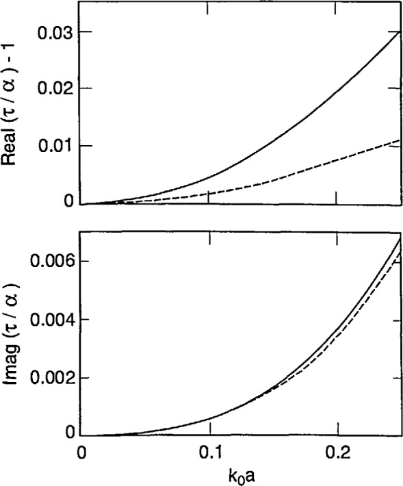
Equations (46a) and (46b) tell us that strong forms incorporate finite-size effects meaningfully, while the weak forms do so trivially. This conclusion is reinforced by Figs. 2–4 that show plots of τ/α versus the normalized radius k₀a of an electrically small sphere for ϵ_r = 1.5, 2.5 and 4.0. In these figures we have ensured that the maximum value of k₀a|ϵ_r^1/2| is about 0.5. We observe – not surprisingly – that τ is complex while α is purely real for these input parameters. Furthermore, in all three figures the ratio |τ/α| lies between 1.02 and 1.03 when k₀a|ϵ_r^1/2| ≅ 0.5; while τ/α = 1 for k₀a = 0, of course. Similar conclusions can be drawn from Fig. 5, wherein the calculations of τ/α have been reported for a lossy dielectric sphere with ϵ_r = 3.75 + 0.25i. These figures highlight the understanding on finite-size effects drawn from Eqs. (46a, b), and it follows that coarser partitioning of V_int may be acceptable when S-CDM/S-MOM is used than when W-CDM/W-MOM is used. These thoughts can be validated by careful examination of the graphs recently published by Ku [19].

Fig. 2.

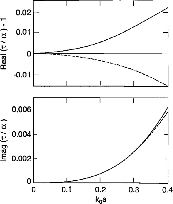
Functions [τ/α − 1] (solid lines) and [τ_DB/α − 1] (dashed lines) as functions of the size parameter k₀a of a spherical sub-region whose relative permittivity ϵ_r = 1.5; the Mossotti-Clausius polarizability α = 4πa³ ϵ₀(ϵ_r − 1)/(ϵ_r + 2).

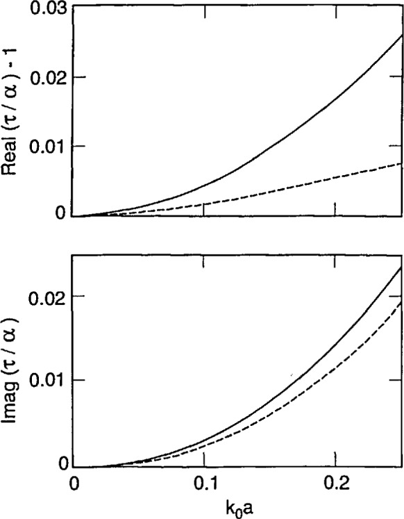
Fig. 3.

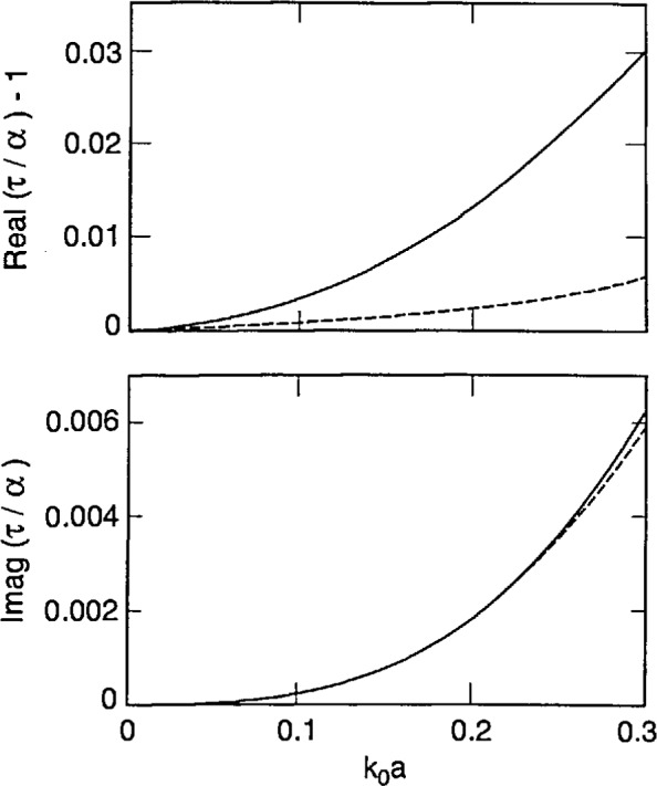
Same as Fig. 2, but ϵ_r = 2.5.

Fig. 4.

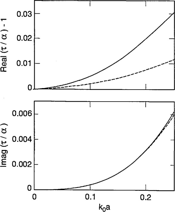
Same as Fig. 2, but ϵ_r = 4.0.

Fig. 5.

Same as Fig. 2, but ϵ_r = 3.75 + 0.25i.

The strong forms discussed above are not the only way of introducing finite-size effects, there being at least two more CDM algorithms available for that purpose. As alluded to earlier, Draine [48] replaced the Mossotti-Clausius polarizability by

$$\begin{array}{cc}{\tau }_{\mathrm{D}}=\mathit{\alpha }/\{1-(i/6\mathit{\pi }{ϵ}_0){{\mathit{k}}_0}^3\mathit{\alpha }\}.& [\text{D-CDM}]\end{array}$$ (47)

However, τ_D is fully contained in τ, as we have seen in Eq. (43); and τ_D approaches α as the size parameter k₀a becomes vanishingly small.

The second source for the incorporation of finite-size effects has been the Lorentz-Mie-Debye analysis for scattering by a dielectric sphere [46]. The electromagnetic field scattered by any object can be described in terms of a multipole expansion [49]. With inspiration from Doyle [50], Dungey and Bohren [51] introduced finite-size effects in the CDM by using the lowest order Mie coefficient – corresponding to the electric dipole term of the mutipole expansion – for the polarizability in place of the Mossotti-Clausius polarizability α. Thus,

$$\begin{array}{l}{\tau }_{\text{DB}}=(i6\pi {ϵ}_0/{{\mathit{k}}_0}^3)\\ \frac{[{{ϵ}_{\mathrm{r}}}^{1/2}\psi ({\mathit{k}}_{0}a{{ϵ}_r}^{1/2})\partial \psi ({\mathit{k}}_{0}a)-\psi ({\mathit{k}}_{0}a)\partial \psi ({\mathit{k}}_{0}a{{ϵ}_{\mathrm{r}}}^{1/2})]}{[{{ϵ}_{\mathrm{r}}}^{1/2}\psi ({\mathit{k}}_{0}a{{ϵ}_{\mathrm{r}}}^{1/2})\partial \zeta ({\mathit{k}}_{0}a)-\zeta ({\mathit{k}}_{0}a)\partial \psi ({\mathit{k}}_{0}a{{ϵ}_{\mathrm{r}}}^{1/2})]}[\text{DB-CDM}]\end{array}$$ (48)

was used in [47], with ψ(β) = β⁻¹ sin(β) − cos(β), ∂ψ(β) = dψ/df/dβ, ζ(β) = − (1 + i/β) exp(iβ), and ∂ζ(β) = dζ/dβ.

Using Eq. (48), it can be shown that τ_DB approaches α as the normalized radius k₀a becomes vanishingly small. This is also borne out in Figs. 2–5, wherein the computed values of τ_DB/α are compared with those of τ/α as functions of the normalized radius k₀a for ϵ_r = 1.5, 2.5, 4.0 and 3.75 + 0.2i. The general behavior of τ_DB is the same as of τ: (i) τ_DB is complex even for purely real ϵ_r and (ii) the ratio |τ_DB/α| lies between 0.99 and 1.01 when k₀a |ϵ_r^1/2| ≅ 0.5 in these figures. A more remarkable observation is that |1 − τ_DB/α| ≤ |1 − τ/α|; in other words, τ_DB is closer to the Mossotti-Clausius polarizability α than τ is.

Draine [48] and Dungey and Bohren [51] concluded from their numerical investigations that D-CDM and DB-CDM, respectively, generally provide scattering results superior to those from W-CDM. This does not come as a surprise because the self-terms in W-CDM (or W-MOM) are estimated with the least accuracy. On the other hand, although it is difficult to provide general enough conclusions for the adequacy of either D-CDM or DB-CDM vis-a-vis that of the S-CDM/S-MOM, it is safe to state that any claims of superiority – based purely on the estimation of some gross parameter, such as the total scattering cross-section – are debatable. Indeed, the only good way of deciding on the superiority of S-CDM, D-CDM or DB-CDM is by making calculations for the specific problem under consideration: The scatterer region should be subdivided into different numbers of subregions, and computed data from the various algorithms for different partitioning schemes compared for the property of interest [52–54].

The refractive index of soot at visible frequencies has been measured by a variety of experimental techniques, and has been found to be dependent on the source materials [55]. We conclude with calculations of τ/α and τ_DB/α for ϵ_r = 2.40 + 2.38i, corresponding to a complex refractive index of 1.7 + 0.7i, in Fig. 6. It is not difficult to gather from this figure that conclusions drawn in the previous paragraphs of this section apply to light scattering by soot agglomerates.

Fig. 6.

Same as Fig. 2, but ϵ_r = 2.40 + 2.38i.

Glossary

0

Null vector

0

Null dyadic

a

Radius of a spherical subregion

a, b, d₁, d₂

Arbitrary vectors

a_m

(1/2) × maximum linear cross-sectional dimension of the sub-region V_m

A_km

Dyadic kernel for the MOM equations

Å_kk, Á_kk

Self-terms when MOM is used with spherical subregions

b

Side of a cubical subregion

B(x)

Magnetic flux density (weber per square meter)

D(x)

Electric flux density (coulomb per square meter)

e_inc

Electric field intensity amplitude of an incident plane wave

E(x)

Electric field intensity (volt per meter)

^(m)E_exc(x)

Electric field intensity exciting the subregion V_m

E_cxc,m

= ^(m)E_exc(X_m)

E_inc(x)

Incident electric field intensity

E_m

Electric field intensity at x_m

E_sca(x)

Scattered electric field intensity

F_sca(u_s)

Far-zone scattering amplitude in the direction u_s

G(x, x′)

Free space dyadic Green’s function

G_km

= G(x_k, x_m)

H(x)

Magnetic field intensity (ampere per meter)

H_sca(x)

Scattered magnetic field intensity

i

= (−1)^1/2

I

Identity dyadic

J(x)

Electric current density (ampere per cubic meter)

J_m

= J(x_m)

J_cond(x)

Conduction current density (ampere per cubic meter)

J_pol(x)

Polarization current density (ampere per cubic meter)

k₀

Free space wavenumber (inverse meter)

L_m, M_m, T_m

Depolarization dyadics for the three-dimensional subregion V_m

M

Total number of subregions

p_m

Electric dipole moment equivalent to the subregion V_m

P_abs

Time-averaged absorbed power

P_sca

Time-averaged scattered power

P_ext

Time-averaged extinguished power

Q_km

Dyadic kernel for the CDM equations

S_m

Closed surface of the three-dimensional subregion V_m

t

Time (seconds)

t_m

Polarizability dyadic of the subregion V_m

u_s

Unit vector denoting direction in the far zone

u_inc

Unit vector denoting propagation direction of an incident plane wave

V_ext

Three-dimensional region external to the scatterer

V_int

Three-dimensional region occupied by the scatterer

V_m

Three-dimensional subregion

x

Three-dimensional position vector (meter)

x_m

Distinguished point inside the subregion V_m

X_km

x_k-x_m

α

Mossotti-Clausius polarizability scalar of a spherical subregion

α_m

Mossotti-Clausius polarizability scalar of the m-th spherical subregion

δ_km

Kronecker delta

δ(x–x′)

Dirac delta

ϵ₀

Permittivity of free space (= 8.854 × 10⁻¹² farad per meter)

ϵ_r

Relative permittivity

ϵ_r(x)

Relative permittivity of dielectric matter occupying V_int

ϵ_r, _m

Relative permittivity of dielectric matter of the subregion V_m

η₀

Intrinsic impedance of free space (= 120 π ohm)

Λ

= [(1 − ik₀a) exp(ik₀a) − 1]

λ

= Wavelength in free space (= 2π/k₀)

μ₀

Permeability of free space (= 4π × 10⁻⁷

ω

Circular frequency (radian per second)

Ω

Solid angle

τ

Polarizability scalar of a spherical subregion

τ_m

Polarizability scalar of the m-th spherical subregion

τ_D

Draine’s polarizability scalar of a spherical subregion

τ_DB

Dungey-Bohren polarizability scalar of a spherical subregion

ν_m

Volume of the subregion V_m (cubic meter)

ψ(β)

A Riccati-Bessel function of argument β

ζ(β)

A Riccati-Hankel function of argument β

Biography

About the authors: Akhlesh Lakhtakia is Associate Professor of Engineering Science and Mechanics at the Pennsylvania State University. George W. Mulholland is Research Chemist and Group Leader, Smoke Dynamics Research Group at NIST. The National Institute of Standards and Technology is an agency of the Technology Administration, U.S. Department of Commerce.

10. Appendix A. The Volume Integral Equation for the Electric Field

The free space Green's function G(x,x′) satisfies the dyadic differential equation

$$\begin{array}{c}\nabla \times \nabla \times \mathbf{G}(\mathit{x},{\mathit{x}}^{\prime })-{{\mathit{k}}_0}^2\mathbf{G}(\mathit{x},{\mathit{x}}^{\prime })=\\ \mathbf{I}\delta (\mathit{x},-{\mathit{x}}^{\prime }),\end{array}$$ (A1-1)

where δ(x−x') is the Dirac delta function. Since J(x′) is not a function of x, it follows that ∇ × [G(x,x′) · J(x′)] = [∇ × G(x, x′)] · J(x′); hence,

$$\begin{array}{c}\nabla \times \nabla \times [\mathbf{G}(\mathit{x},{\mathit{x}}^{\prime })\cdot \mathit{J}({\mathit{x}}^{\prime })]-\\ {{\mathit{k}}_0}^2[\mathbf{G}(\mathit{x},{\mathit{x}}^{\prime })\cdot \mathit{J}({\mathit{x}}^{\prime })]=\mathbf{I}\cdot \mathit{J}({\mathit{x}}^{\prime })\delta (\mathit{x}-{\mathit{x}}^{\prime }).\end{array}$$ (A1-2)

We multiply both sides of this equation by iωμ₀ and integrate over all x′ to get

$$\begin{array}{c}(\nabla \times \nabla \times \mathbf{I}-{{\mathit{k}}_0}^2\mathbf{I})\cdot {\displaystyle {\iiint }_{|{\mathit{x}}^{\prime }|\le \infty }{\mathrm{d}}^3{\mathit{x}}^{\prime }}\\ [i\omega {\mu }_0\mathbf{G}(\mathit{x},{\mathit{x}}^{\prime })\cdot \mathit{J}({\mathit{x}}^{\prime })]=\\ i\omega {\mu }_0{\displaystyle {\iiint }_{|{\mathit{x}}^{\prime }|\le \infty }{\mathrm{d}}^3{\mathit{x}}^{\prime }\mathit{J}({\mathit{x}}^{\prime })\delta (\mathit{x},{\mathit{x}}^{\prime })},\end{array}$$ (A1-3)

whence,

$$\begin{array}{c}(\nabla \times \nabla \times \mathbf{I}-{{\mathrm{k}}_0}^2\mathbf{I})\cdot {\displaystyle {\iiint }_{|{\mathit{x}}^{\prime }|\le \infty }{\mathrm{d}}^3{\mathit{x}}^{\prime }}\\ [i\omega {\mu }_0\mathbf{G}(\mathit{x},{\mathit{x}}^{\prime })\cdot \mathit{J}({\mathit{x}}^{\prime })]=i\omega {\mu }_0\mathit{J}(\mathit{x}).\end{array}$$ (A1-4)

Now by comparing Eqs. (7) and (A1-4), it is not too arduous to convince ourselves that

$$\begin{array}{c}\mathit{E}(\mathit{x})=i\omega {\mu }_0{\displaystyle {\iiint }_{|{\mathit{x}}^{\prime }|\le \infty }{\mathrm{d}}^3{\mathit{x}}^{\prime }[\mathbf{G}(\mathit{x},{\mathit{x}}^{\prime })\cdot \mathit{J}({\mathit{x}}^{\prime })]};\\ 0\le |\mathit{x}|\le \infty .\end{array}$$ (A1-5)

Remembering that for the present purposes J(x) is null everywhere except in V_int, we next obtain

$$\begin{array}{c}\mathit{E}(\mathit{x})=i\omega {\mu }_0{\displaystyle {\iiint }_{V_{\mathrm{int}}}{\mathrm{d}}^3{\mathit{x}}^{\prime }[\mathbf{G}(\mathit{x},{\mathit{x}}^{\prime })\cdot \mathit{J}({\mathit{x}}^{\prime })]};\\ \mathit{x}\in V_{\mathrm{int}}+V_{\text{ext}}.\end{array}$$ (A1-6)

The solution of every linear differential equation can be divided into two parts: the particular solution that depends on the forcing function, J(x) being the forcing function here, and the complementary function that holds when the forcing function is identically zero everywhere. The right side of Eq. (A1-6) is the particular solution of Eq. (7), which has the complementary function E_inc(x) satisfying

$$\begin{array}{c}\nabla \times \nabla \times {\mathit{E}}_{\text{inc}}(\mathit{x})-{{\mathit{k}}_0}^2{\mathit{E}}_{\text{inc}}(\mathit{x})=\mathit{0};\\ \mathit{x}\in V_{\mathrm{int}}+V_{\text{ext}}.\end{array}$$ (A1-7)

Hence, the complete solution of Eq. (7) is

$$\begin{array}{c}\mathit{E}(\mathit{x})={\mathit{E}}_{\text{inc}}(\mathit{x})+i\omega {\mu }_0{\displaystyle {\iiint }_{V_{\mathrm{int}}}{\mathrm{d}}^3{\mathit{x}}^{\prime }}\\ [\mathbf{G}(\mathit{x},{\mathit{x}}^{\prime })\cdot \mathit{J}({\mathit{x}}^{\prime })];\mathit{x}\in V_{\mathrm{int}}+V_{\text{ext}},\end{array}$$ (A1-8)

which can be easily re-expressed as Eq. (8a).

11. Appendix B. The Self-Integral

The integral under consideration is given as

$$\mathit{a}({\mathit{x}}_0)={\displaystyle {\iiint }_V{\mathrm{d}}^3{\mathit{x}}^{\prime }\mathbf{G}({\mathit{x}}_0,{\mathit{x}}^{\prime })\cdot \mathit{b}({\mathit{x}}^{\prime })},$$ (A2-1)

where V is the region bounded by the surface S, as shown in Fig. 7, G(x, x′) is given by Eq. (8c), and the point x₀ lies inside V. Because G(x, x′) is of the order 1/|x − x′|³ for |x − x′| ≅ 0, and becomes singular at x = x′, this integral has to be carefully treated.

Fig. 7.

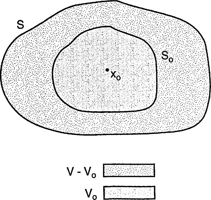
For the evaluation of the integral in Eq. (A2-1) when x₀ ∈ V and x′ ∈ V.

As shown by Fikioris [56], we can transform Eq. (A2-1) to

$$\begin{array}{c}\mathit{a}({\mathit{x}}_0)={\displaystyle {\iiint }_{V-V_0}{\mathrm{d}}^3{\mathit{x}}^{\prime }[\mathbf{G}({\mathit{x}}_0,{\mathit{x}}^{\prime })\cdot \mathit{b}({\mathit{x}}^{\prime })]}+\\ {\displaystyle {\iiint }_{V_0}{\mathrm{d}}^3{\mathit{x}}^{\prime }[\mathbf{G}({\mathit{x}}_0,{\mathit{x}}^{\prime })\cdot \mathit{b}({\mathit{x}}^{\prime })-{\mathbf{G}}_{\mathbf{s}}({\mathit{x}}_0,{\mathit{x}}^{\prime })\cdot \mathit{b}({\mathit{x}}_0)]}\\ -(1/{{\mathit{k}}_0}^2){\displaystyle {\iint }_{{\mathrm{S}}_0}{\mathrm{d}}^2{x}^{\prime }{u_n}^{\prime }}\\ [({\mathit{x}}^{\prime }-{\mathit{x}}_0)/4\pi {|{\mathit{x}}^{\prime }-{\mathit{x}}_0|}^3]\cdot \mathit{b}({\mathit{x}}_0),\end{array}$$ (A2-2)

where

$${\mathbf{G}}_{\mathit{s}}(\mathit{x},{\mathit{x}}^{\prime })=(1/{{\mathit{k}}_0}^2)\nabla \nabla [1/4\pi |\mathit{x}-{\mathit{x}}^{\prime }|]$$ (A2-3)

is an auxiliary dyadic related to the Green’s function for Poisson’s equation [10]; V₀ is an exclusionary region bounded by the surface S₀, as shown in Fig. 7; u_n is the unit normal to S₀, pointing away from V₀, at the point x′ ∈ S₀. The exclusionary region V₀ should be small but not necessarily infinitesimal, and it must be wholly contained within V. Moreover, there is no requirement that S₀ be a miniature copy of S.

The use of the long-wavelength approximation b(x)≅b(x₀) for all x ∈ V reduces Eq. (A2-2) to

$$\begin{array}{c}\mathit{a}({\mathit{x}}_0)\cong {\displaystyle {\iiint }_{V-V_0}{\mathrm{d}}^3{\mathit{x}}^{\prime }[\mathbf{G}({\mathit{x}}_0,{\mathit{x}}^{\prime })\cdot \mathit{b}({\mathit{x}}_0)]+}\\ {\displaystyle {\iiint }_{V_0}{\mathrm{d}}^3{\mathit{x}}^{\prime }\{[\mathbf{G}({\mathit{x}}_0,{\mathit{x}}^{\prime })-{\mathbf{G}}_{\mathit{s}}({\mathit{x}}_0,{\mathit{x}}^{\prime })]\cdot \mathit{b}({\mathit{x}}_0)\}}\\ -(1/{{\mathit{k}}_0}^2){\displaystyle {\iint }_{{\mathrm{S}}_0}{\mathrm{d}}^2{\mathit{x}}^{\prime }{{\mathit{u}}_n}^{\prime }[({\mathit{x}}^{\prime }-{\mathit{x}}_0)/}\\ 4\pi {|{\mathit{x}}^{\prime }-{\mathit{x}}_0|}^3]\cdot \mathit{b}({\mathit{x}}_0).\end{array}$$ (A2-4)

Since V is electrically small, but V₀ need not be infinitesimal, we set V = V₀ and S = S₀ to have

$$\mathit{a}({\mathit{x}}_0)\cong [\mathbf{M}-(1/{{\mathit{k}}_0}^2)\mathbf{L}]\cdot \mathit{b}({\mathit{x}}_0),$$ (A2-5a)

where

$$\mathbf{M}={\displaystyle {\iiint }_V{\mathrm{d}}^3{\mathit{x}}^{\prime }[\mathbf{G}({\mathit{x}}_0,{\mathit{x}}^{\prime })-{\mathbf{G}}_{\mathit{s}}({\mathit{x}}_0,{\mathit{x}}^{\prime })]},$$ (A2-5b)

$$\mathbf{L}={\displaystyle {\iint }_S{\mathrm{d}}^2{\mathit{x}}^{\prime }{{\mathit{u}}_n}^{\prime }[({\mathit{x}}^{\prime }-{\mathit{x}}_0)/4\pi {|{\mathit{x}}^{\prime }-{\mathit{x}}_0|}^3]}.$$ (A2-5c)

The evaluation of M can be accomplished numerically for regions of different shapes using the coordinate-free (i.e., non-indicial) representations [24, Chap. 9]

$$\begin{array}{c}\mathbf{G}(\mathit{x},{\mathit{x}}^{\prime })=[(\mathbf{I}-{\mathit{u}}_X{\mathit{u}}_X)+(i/{\mathit{k}}_0|\mathbf{X}|)(1+i/{\mathit{k}}_0|\mathbf{X}|)\\ (\mathbf{I}-3{\mathit{u}}_X{\mathit{u}}_X)][\exp (i{\mathit{k}}_0|\mathit{x}-{\mathit{x}}^{\prime }|)/4\pi |\mathit{x}-{\mathit{x}}^{\prime }|];\\ |\mathit{X}|\ne 0,\end{array}$$ (A2-6a)

$$\begin{array}{c}{\mathbf{G}}_{\mathit{s}}(\mathit{x},{\mathit{x}}^{\prime })={(i/{\mathit{k}}_0|\mathit{X}|)}^2(\mathbf{I}-3{\mathit{u}}_X{\mathit{u}}_X)]/4\pi |\mathit{X}|;\\ |\mathit{X}|\ne 0,\end{array}$$ (A2-6b)

where X = x−x′ and u_x = X/|X|. The evaluation of the depolarization dyadic L is equally easy on a digital computer, and analytical expressions for L are available for the quite general ellipsoidal shapes [57].

If V is extremely small in electrical size, the simplification

$$\mathit{a}({\mathit{x}}_0)\cong (1/{{\mathit{k}}_0}^2)\mathbf{L}\cdot \mathit{b}({\mathit{x}}_0)$$ (A2-7)

is permissible and leads to the weak forms of the MOM and the CDM.

12. Appendix C: The Self-Dyadics for Spherical and Cubical Regions

Let the region V in Appendix B be a sphere with radius a and center at x₀. Without loss of generality due to the translational invariance of the right sides of Eqs. (A2-6a, b), we set x₀= 0. Furthermore, we set x′ = r′ (u₁ sinθ′ cosϕ′ + u₂ sinθ′ sinϕ′ + u₃ cosθ′), where |x′| = r′, (u₁, u₂, u₃) is the triad of cartesian unit vectors, while (r′, θ′, ϕ′) represent the corresponding spherical coordinate system located at the center of the sphere. Hence,

$$\begin{array}{c}{\displaystyle {\iiint }_V{\mathrm{d}}^3{\mathit{x}}^{\prime }\{\cdot \}\equiv {\displaystyle {\int }_0^a\mathrm{d}{r}^{\prime }{r^{\prime }}^2{\displaystyle {\int }_0^{\pi }\mathrm{d}{\theta }^{\prime }\sin {\theta }^{\prime }{\displaystyle {\int }_0^{2\pi }\mathrm{d}{\varphi }^{\prime }\{\cdot \}}}}},\\ {\displaystyle {\iint }_S{\mathrm{d}}^2{\mathit{x}}^{\prime }\{\cdot \}\equiv a^2{\displaystyle {\int }_0^{\pi }\mathrm{d}{\theta }^{\prime }\sin {\theta }^{\prime }{\displaystyle {\int }_0^{2\pi }\mathrm{d}{\varphi }^{\prime }\{\cdot \}}}}.\end{array}$$

Now,

$$\begin{array}{c}{\displaystyle {\int }_0^{\pi }\mathrm{d}{\theta }^{\prime }\sin {\theta }^{\prime }{\displaystyle {\int }_0^{2\pi }\mathrm{d}\varphi {\mathit{u}}_x{\mathit{u}}_x=}}\\ {\displaystyle {\int }_0^{\pi }\mathrm{d}{\theta }^{\prime }\sin {\theta }^{\prime }{\displaystyle {\int }_0^{2\pi }\mathrm{d}{\varphi }^{\prime }\{({\mathit{u}}_1\sin {\theta }^{\prime }\cos {\varphi }^{\prime }}}+\\ {\mathit{u}}_2\sin {\theta }^{\prime }\sin {\varphi }^{\prime }+{\mathit{u}}_3\cos {\theta }^{\prime })({\mathit{u}}_1\sin {\theta }^{\prime }\cos {\varphi }^{\prime }+{\mathit{u}}_2\\ \sin {\theta }^{\prime }\sin {\varphi }^{\prime }+{\mathit{u}}_3\cos {\theta }^{\prime })\}=\\ \pi {\displaystyle {\int }_0^{\pi }\mathrm{d}{\theta }^{\prime }\sin {\theta }^{\prime }\{({\mathit{u}}_1{\mathit{u}}_1+{\mathit{u}}_2{\mathit{u}}_2){\sin }^2\theta +2{\mathit{u}}_3{\mathit{u}}_3{\cos }^2{\theta }^{\prime }\}}=\\ (4\pi /3)({\mathit{u}}_1{\mathit{u}}_1+{\mathit{u}}_2{\mathit{u}}_2+{\mathit{u}}_3{\mathit{u}}_3)=(4\pi /3)\mathbf{I},\end{array}$$ (A3-1)

and

$${\displaystyle {\int }_0^{\pi }\mathrm{d}{\theta }^{\prime }\sin {\theta }^{\prime }{\displaystyle {\int }_0^{2\pi }\mathrm{d}{\varphi }^{\prime }\mathbf{I}=4\pi \mathbf{I}}}$$ (A3-2)

likewise. It follows that

$$\begin{array}{c}\mathbf{M}{|}_{\text{sphere}}={\displaystyle {\int }_0^a\mathrm{d}{r}^{\prime }{r^{\prime }}^2{\displaystyle {\int }_0^{\pi }\mathrm{d}{\theta }^{\prime }\sin {\theta }^{\prime }{\displaystyle {\int }_0^{2\pi }\mathrm{d}{\varphi }^{\prime }}}}\\ \{[\mathbf{G}(\mathit{0},{\mathit{x}}^{\prime })-{\mathbf{G}}_{\mathit{s}}(\mathit{0},{\mathit{x}}^{\prime })]\}\\ ={\displaystyle {\int }_0^a\mathrm{d}{r}^{\prime }{r^{\prime }}^2[(2\mathbf{I}/3)\exp (i{\mathit{k}}_0{r}^{\prime })/r^{\prime }]}\\ =\mathbf{I}(2/3{{\mathit{k}}_0}^2)[(1-i{\mathit{k}}_{0}a)\exp (i{\mathit{k}}_{0}a)-1].\end{array}$$ (A3-3)

In order to evaluate L for a spherical region, we note that u_n′ = x′/|x′| where x′ ∈ S; ergo, |x′| = a, and

$$\begin{array}{c}\mathbf{L}{|}_{\text{sphere}}=a^2{\displaystyle {\int }_0^{\pi }\mathrm{d}{\theta }^{\prime }\sin {\theta }^{\prime }{\displaystyle {\int }_0^{2\pi }\mathrm{d}{\varphi }^{\prime }}}\\ \{{{\mathit{u}}_n}^{\prime }{\mathit{x}}^{\prime }/4\pi a^3\}=(1/4\pi )\\ {\displaystyle {\int }_0^{\pi }\mathrm{d}{\theta }^{\prime }\sin {\theta }^{\prime }{\displaystyle {\int }_0^{2\pi }\mathrm{d}{\varphi }^{\prime }\{({\mathit{u}}_1\sin {\theta }^{\prime }\cos {\varphi }^{\prime }+}}\\ {\mathit{u}}_2\sin {\theta }^{\prime }\sin {\varphi }^{\prime }+{\mathit{u}}_3\cos {\theta }^{\prime })({\mathit{u}}_1\sin {\theta }^{\prime }\cos {\varphi }^{\prime }+\\ {\mathit{u}}_2\sin {\theta }^{\prime }\sin {\varphi }^{\prime }+{\mathit{u}}_3\cos {\theta }^{\prime })\}\\ =(1/4\pi )(4\pi /3)\mathbf{I}=(1/3)\mathbf{I},\end{array}$$ (A3-4)

after using Eq. (A3-1).

If the region V in Appendix B were to be a cube of side b, we would get

$$\mathbf{L}{|}_{\text{cube}}=(1/3)\mathbf{I},$$ (A3-5)

the same as that for a sphere. No expression exists for the dyadic M for a cube in closed form; however, it is commonplace in MOM practice to use the value for an equivoluminal sphere. Thus,

$$\begin{array}{c}\mathbf{M}{|}_{\text{cube}}\cong \mathbf{I}(2/3{{\mathit{k}}_0}^2)\{[1-i{\mathit{k}}_{0}b{(3/4\pi )}^{1/3}]\\ \exp [i{\mathit{k}}_{0}b{(3/4)}^{1/3}]-1\},\end{array}$$ (A3-6)

because [(3/4π)^1/3 b] is the radius of a sphere having the same volume as the cube of side b.