Robust Cell Detection of Histopathological Brain Tumor Images Using Sparse Reconstruction and Adaptive Dictionary Selection

Abstract

Successful diagnostic and prognostic stratification, treatment outcome prediction, and therapy planning depend on reproducible and accurate pathology analysis. Computer aided diagnosis (CAD) is a useful tool to help doctors make better decisions in cancer diagnosis and treatment. Accurate cell detection is often an essential prerequisite for subsequent cellular analysis. The major challenge of robust brain tumor nuclei/cell detection is to handle significant variations in cell appearance and to split touching cells. In this paper, we present an automatic cell detection framework using sparse reconstruction and adaptive dictionary learning. The main contributions of our method are: 1) A sparse reconstruction based approach to split touching cells; 2) An adaptive dictionary learning method used to handle cell appearance variations. The proposed method has been extensively tested on a data set with more than 2000 cells extracted from 32 whole slide scanned images. The automatic cell detection results are compared with the manually annotated ground truth and other state-of-the-art cell detection algorithms. The proposed method achieves the best cell detection accuracy with a F₁ score = 0.96.

I. Introduction

Brain tumor is one of the leading cancers which has increasing cases recently [1]. Successful diagnostic and prognostic stratification, treatment outcome prediction, and therapy planning depend on reproducible and accurate analysis of digitized histopathological specimens [2], [3]. Current manual analysis of histopathological slides is not only laborious, but also subject to inter-observer variability. Computer-aided diagnosis (CAD) systems have attracted broad interests [4], [5]. In CAD systems, cell detection is often a prerequisite step for cellular level morphological analysis [6], [7].

The accurate cell detection in histopathological images has attracted a wide range of interests recently. A brief summary on nuclei detection and segmentation is presented in [5]. Distance transform based methods have been used to detect seeds (cells) in clustered objects. However, it may not work well for tightly or densely clustered cells. Endeavors combining geometric and intensity information have been proposed to improve the distance transform methods [8]. Despite of the improvement, this method is flawed in high false detection rate. Later, to reduce the false detection, mutual proximity information is exploited to filter out the false seeds [9]. In order to handle cell touching/occlusion, marker-based watershed approaches [10], [11], [12] are widely utilized to locate and split touching cells. In [13], a variant of marker-controlled watershed generating marker from H-minima transform of nuclei shape is investigated. The H-value is derived from the fitting accuracy between the ellipses and nuclei contours. Although H-minima based methods aim to reduce the false detection, they provide only limited robustness to the cells with heterogeneous intensity. In [14], an adaptive H-minima transform is proposed in which markers are detected within connected components obtained by inner distance transform. A supervised marker-controlled watershed algorithm is proposed in [15] in which neighboring local minima are merged based on features extracted from the valley lines between them. This method works well with cells without intracellular heterogeneity. However, false valley lines could be created in the case of intracellular heterogeneity. In [16], a flood level-based watershed algorithm is reported to split overlapping nuclei on RNAi fluorescent cellular images. Their method exploited the cues from different channels of the fluorescent images. Those cues are unavailable in our data. A gradient-weighted watershed algorithm [17] followed by a hierarchical merging tree is presented to separate touching cells. Nevertheless, in the above method intra-class shape variation is not considered. In [18], touching cells and stand-alone cells are classified based on geometric features. Then the conventional watershed method is improved by a subregion merging mechanism and a Laplacian-of-Gaussian (LOG) filter. LoG based methods are usually sensitive to large variations in cell size and the absence of obvious cell boundaries.

Cell detection can also be formulated into a graph cut problem [19]. In [20], cell detection is formulated into a normalized graph cut problem over a weighted graph [21]. Another method applying graph-cut algorithm to an image preprocessed by multiscale LOG filtering is reported in [22]. In [23], the foreground is delineated via multi-reference graph cut. The nuclei separation is conducted through geometric reasoning based on concave points. One drawback of this method is its reliance on robust concave point detection that is challenging in the presence of tightly touching cells or high heterogeneity. Some other graph-based methods can be found in [24], [25]. In general, graph-cut based methods are i) sensitive to large variations in shape; ii) and not robust to the absence of the obvious cell boundaries. In [26], markers are derived by a modified ultimate erosion process and a Gaussian mixture model on B-splines is utilized to infer the object shapes and missing object boundaries. However, the method may not work well on cells with heterogeneous intensity and cluttered background. Recently, a deep learning-based method [27] is applied to mitosis detection and achieves great performance. However, this framework does not apply to touching cells which are very common in our dataset.

Some recent works exploit the cues in cell structure and shape symmetry to tackle touching cell problem. Radial voting based methods [28], [29], [30] are proposed to locate the centers of cells with a major assumption on round shaped cells. In [31], radial symmetry is applied to detect the touching cells. The touching cells are separated based on concave points. Fast radial symmetry transform is used for nuclei detection followed by marker-controlled watershed in [32]. These radial symmetry/voting based methods largely rely on the roundness assumption of the cell shape that is not valid in our data set. A cell splitting method based on ellipse fitting using concave points information is reported in [33]. Su et al. [34] propose to learn a classifier to refine the cell detection results obtained by ellipse fitting.

The major challenges in cell detection for the brain tumor data set include i) shape variation, ii) cell touching or overlapping, and iii) heterogeneous intracellular intensity, and iv) weak cell boundaries. Although the existing methods are able to handle some of these challenges, they fail in simultaneously addressing all of them. Therefore the accurate cell detection in brain tumor histopathological images remains to be a challenging problem.

Sparse representation has been successfully applied to image classification, object recognition, and image segmentation [35], [36], [37]. Yu et al. [38] have found that sparse coding with locality constraint (LCC) produces better reconstruction results. However, solving LCC is computationally expensive due to its iterative optimization procedure [39]. An efficient locality-constrained linear coding (LLC) is proposed in [40]. In LLC, the desirable properties of sparsity is preserved while locality constraint is treated in favor of sparsity. The problem can be efficiently solved by performing a K-nearest neighbor (KNN) search and then computing an analytical solution to a constrained least square fitting problem.

Following the above research line, there is an emerging trend of applying patch dictionary and sparsity based methods to pathology image analysis. Kårsnäs et al. [41] propose to separate the foreground (nuclei) from the background using a patch dictionary learned through a modified vector quantization algorithm. A probability map is obtained through pixel-wise labeling based on the learned patch dictionary and its corresponding label dictionary. Each pixel is assigned a label based on the similarity between the patch centered on the pixel and the dictionary patches. Touching cells are split by the marker controlled watershed algorithm and a complement to the distance transform of a pixel level probability map. The proposed method is not applicable to our data, because a local patch does not contain sufficient information for discerning a real cell boundary and an edge in the background, especially when contrast changes occur. In [42], Sparse shape modeling is coupled with a repulsive balloon snake deformable model for robust segmentation of cells with intracellular inhomogeneity. Sparse learning methods are also observed in the field of classification of sections in histology images [43], [44], [45]. In spite of the above endeavors, the potential advantage of sparse coding for cell detection has not been systematically studied.

In this paper, we propose a novel automatic cell detection algorithm (Figure 1) using adaptive dictionary learning and sparse reconstruction with trivial templates. The algorithm consists of the following steps: 1) A set of training image patches is collected from images of different brain tumor patients at different stages. K-selection [46] is then applied on this dataset to learn a compact cell library. 2) Given a testing image, a testing image specific dictionary is generated by searching in the learned library for similar cells. Cosine distance based on local steering kernel features is employed as the similarity measurement [47], [48]. 3) The sparse reconstruction using trivial templates is applied to handle touching cells. A probability map is obtained by comparing the sparsely reconstructed image patch to each testing window. 4) A weighted mean-shift clustering is used to generate the final cell detection results.

Fig. 1.

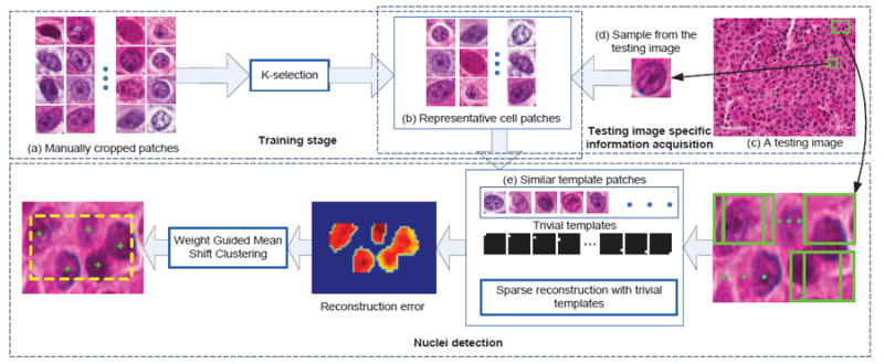
An overview of the proposed algorithm. There are three components, including training stage, testing image specific information acquisition, and cell detection using sparse reconstruction with trivial templates. In training stage, a set of representative patches (b) are selected from thousands of manually cropped single-cell patches (a). In the testing image specific information acquisition, for a given testing image (c), a sample patch (d) is cropped and used to find similar patches (e) from the representative patches (b) to form the dictionary. Cell detection is performed based on sparse representation using trivial templates.

The rest of this paper is organized as the following: Section II describes the proposed framework. Section III evaluates the performance of the proposed system. Section IV concludes this paper.

II. Method

A. Dictionary Learning

At training stage, we manually crop many image patches, and each patch contains one cell located in the center (Fig. 1 (a)). These image patches form an over-complete dictionary, which is neither robust nor efficient. Considering this factor, we propose to use the K-selection [46] to select a subset of representative patches to build a compact dictionary. In order to further improve the computational efficiency, we only utilize the patches similar to the testing image patches as the dictionary candidates measured by cosine similarity metric [47].

Dictionary Learning Using K-Selection

Each cell patch is represented by a m dimensional vectorized patch by concatenating all the pixel intensities. For N manually-cropped cell patches T = {t_i∣i = 1, 2, … , N} ∈ ℝ^m×N (t_i ∈ ℝ^m), the K-selection algorithm directly chooses a set of most representative patches to create the dictionary B = {b_i∣i = 1, 2, … , K} ∈ ℝ^m×K based on locality-constrained sparse representation. The optimization can be formulated as

$$\begin{array}{l}\underset{{\mathit{b}}_k\in B,{\mathit{x}}_i}{\min }\sum _{i=1}^N{\Vert {\mathit{t}}_i-\sum _{k=1}^K{\mathit{b}}_k{x}_{ik}\Vert }^2+\mathrm{\lambda }{\Vert {\mathit{d}}_i\odot {\mathit{x}}_i\Vert }^2,\\ s.t.{\mathbf{1}}^T{\mathit{x}}_i=1,\forall i,\end{array}$$ (1)

where b_k is the k-th basis patch selected from the original template pool, x_i is the sparse coefficient, and x_ik is the k–th entry of x_i, and d_i is the distance between t_i and the basis vectors, and ☉ denotes element-wise multiplication. The constraint 1^Tx_i = 1, ∀ i, enforces the shift-invariance requirement in LLC.

Equation (1) can be optimized by alternatively updating B or {x_i} by fixing the other. Different than K-SVD [49], dictionary B is updated by replacing one basis with another sample selected from the data set (details can be found in [40] and [46]). The locality constraint (the second term in (1)) ensures a sample t_i is represented only by its neighbors. It guarantees that similar patches are assigned similar sparse codes without losing discriminative powers. Therefore, the selected patches can better represent all the training image patches.

The Generation of The Dictionary For A Specific Testing Image

Given a testing image, we propose to choose a subset of cell patches in the representative cell library for the subsequent sparse coding. Instead of using the entire learned library, this step can reduce the computational complexity. The Local steering kernel (LSK) is used as local features to represent each image patch [50]. Cosine similarity is used to measure the similarity between the testing image patch and the learned dictionary bases. The LSK-based feature descriptor measures the local similarity of a pixel to its neighbors by estimating the shape and size of a canonical kernel. A demonstration of the estimated kernels for different local image structures are shown in Fig. 2.

Fig. 2.

A demonstration of LSK at different regions. The local image structure is encoded by LSK.

We calculate the LSKs of a patch by applying a sliding window with stride 3 to the entire patch. Principal component analysis (PCA) is then applied to extract the low dimensional feature vectors of the local steering kernels for each image patch.

Let v_i and v_j denote the low dimensional features representing two different patches. The cosine similarity D_cos between them is:

$$D_{\mathit{cos}}=\frac{{\mathbf{v}}_i^T{\mathbf{v}}_j}{\Vert {\mathbf{v}}_i\Vert \Vert {\mathbf{v}}_j\Vert }.$$ (2)

The reason that we choose the cosine similarity is because contrast variations often exist in digitized pathology images due to unstable staining, and the cosine similarity is proven to be robust to contrast change [48].

In order to provide rotation invariance, the sample patch is rotated into different orientations. For each rotation, a set of most similar cell patches are selected to be the bases for the subsequent sparse reconstruction. Fig. 3 shows two specific dictionaries given two different query cell patches. Each query sample is rotated in five orientations as shown in the first column. For illustration purpose we show only six retrieved patches in the dictionary for each orientation.

Fig. 3.

A demonstration of the adaptive dictionary generation using two sample patches (a and b). The first column in each panel shows the rotated versions of a sample patch. Each row of the other columns shows the retrieved relevant patches in the learned dictionary.

B. Cell Detection via Sparse Representation with Trivial Templates

In this section, we present the proposed cell detection algorithm based on sparse reconstruction with trivial templates to handle touching cells. Sparse reconstruction error of a sliding window (corresponding to an image patch) over the entire testing image is used to generate a probability map that indicates the presence of cells. The final detection results are obtained by applying weighted mean-shift clustering [51] to the probability map.

Sparse Reconstruction Using Trivial Templates

We assume that cells with similar appearances approximately lie in the same low dimensional subspace. Therefore, a sliding window aligned to a cell should approximately lie in the subspace spanned by the dictionary generated in subsection II-A. In other words, given a learned dictionary B ∈ ℝ^m×q, a sliding window p_ij aligned to a cell at location (i, j) can be linearly represented by B:

$${\mathbf{p}}_{\mathit{ij}}\approx \mathbf{Bc}=c_1{\mathbf{b}}_{\mathbf{1}}+c_2{\mathbf{b}}_{\mathbf{2}}+\cdots +c_q{\mathbf{b}}_{\mathbf{q}}.$$ (3)

If the sliding window is not aligned to the center of the cell, Equation (3) does not hold. To differentiate the tumor cells from background, we propose to measure how closely a sliding window can be approximated by a linear combination of the atom patches from the dictionary:

$${\epsilon }_{\mathit{rec}}=\Vert {\mathbf{p}}_{\mathit{ij}}-\mathbf{Bc}\Vert ,$$ (4)

where ε_rec is the reconstruction error and c is the sparse reconstruction coefficients. It can be computed by sparse optimization:

$$\underset{\mathbf{c}}{\min }{\Vert {\mathbf{p}}_{\mathit{ij}}-\mathbf{Bc}\Vert }^2+\mathrm{\lambda }\Vert \mathbf{d}\odot \mathbf{c}\Vert ,s.t.{\mathbf{1}}^T\mathbf{c}=1,$$ (5)

where d is the distance between the test patch p_ij and the dictionary, and ☉ denotes element-wise multiplication. The second term in (5) enforces the encoding to use only the dictionary atoms near to p_ij.

An input patch containing a cell in its central area can be sparsely reconstructed with relatively small reconstruction error, while a patch that does not have a cell in its center will have relatively large sparse reconstruction error, because such patches do not lie in the subspace spanned by the learned dictionary. To achieve fast encoding, we choose the approximated optimization algorithm presented in [40].

One drawback of Equation (3) is its inability to split touching cells. It is very common for a testing sliding window to contain more than just one cell. For these cases, the appearance of the patch is significantly different from the atom patches in the dictionary. In order to handle this situation (referred as partial occlusion in cell detection), we propose to use the following equation:

$${\mathbf{p}}_{\mathit{ij}}\approx \mathbf{Bc}+\mathbf{e},$$ (6)

where e is an error term used to model the occlusion part. In order to model the non-object region that can occur in arbitrary positions of a testing image patch, a set of unit vectors are used as the bases, as suggested in [52], [35]. Such set of bases are composed of the columns of an identity matrix, thus can represent any vector (with a linear combination) in the corresponding space. Equation (6) can be rewritten as:

$${\mathbf{p}}_{\mathit{ij}}\approx \stackrel{\sim }{\mathbf{B}}\stackrel{\sim }{\mathbf{c}}=[\begin{array}{cc}\mathbf{B}& \mathbf{I}\end{array}]\left[\begin{array}{c}\mathbf{c}\\ \mathbf{e}\end{array}\right],$$ (7)

where the columns of identity matrix I ∈ ℝ^m×m are called trivial templates. Accordingly the reconstruction error ε_rec is modified as:

$${\epsilon }_{\mathit{rec}}=\Vert {\mathbf{p}}_{\mathit{ij}}-\stackrel{\sim }{\mathbf{B}}\stackrel{\sim }{\mathbf{c}}\Vert ,$$ (8)

and Equation (5) can be modified as:

$$\underset{\stackrel{\mathbf{\sim }}{\mathbf{c}}}{\min }{\Vert {\mathbf{p}}_{\mathit{ij}}-\stackrel{\mathbf{\sim }}{\mathbf{B}}\stackrel{\mathbf{\sim }}{\mathbf{c}}\Vert }^2+\mathrm{\lambda }{\Vert \mathbf{d}\odot \mathbf{c}\Vert }^2+\gamma {\Vert \mathbf{e}\Vert }^2,s.t.{\mathbf{1}}^T\stackrel{\mathbf{\sim }}{\mathbf{c}}=1,$$ (9)

where the first term incorporates the trivial templates to model the touching cells and the second term enforces that only local neighbors in the dictionary are used for the sparse reconstruction. The third term controls the contribution of the trivial templates in the reconstruction. A smaller γ encourages more contribution from the trivial templates. Thus better reconstruction. A larger one limits the contribution of the trivial templates. In order to solve the locality-constrained sparse optimization for a given input patch, we first perform a KNN search in the dictionary excluding the trivial templates. The selected nearest neighbor bases together with the trivial templates form a much smaller local coordinate. Next, we solve the sparse reconstruction problem with least square minimization. We demonstrate the reconstruction results of touching cells with and without trivial templates in Fig. 4.

Fig. 4.

A demonstration of the sparse reconstruction with/without trivial templates to handle touching cells. (a) Two sliding windows aligned to cells touching with other cells. (b) The reconstructed patch using only the dictionary patches. (c) The reconstructed patch using trivial templates to model the occlusion parts. (d) Visualization of the first term and the second term (error) in Equation (6). The upper ones are the clean images and the bottom ones are the visualizations of the error terms. As we can see that the reconstructions (b) without trivial templates have higher level of noise and weaker edges. However, the sparse reconstructions using trivial templates (c) are very similar to the original image. In addition, compared to the original patches in (a), it is clear that the clean image in (d) (rows 1 and 3) not only preserves the original shape of the cell, but also removes the touching cells (occlusions). This is due to the contribution of the trivial templates. Using the reconstruction images (c) provides better cell detection results, because it gives much smaller sparse reconstruction errors even there exist occlusions.

The interpretation of why the trivial templates help handling touching/occlusion lies in the comparison between Eq. 5 and Eq. 9. In Eq. 5, since each atom corresponds to one training patch with one single non-touching cell at its center, the atoms can sufficiently represent a testing patch with a centered single non-touching cell, by using Eqs. (3, 5) and exhibiting a low reconstruction error (Eq. 4). However, the patches with touching/occlusion cells exhibit unexpected appearances in the background such that they are not consistent with the dictionary atoms, and thus sparse reconstruction with Eq. 5 could result in larger reconstruction errors. An error term e is introduced in Eq. (6) to model the non-object region. With a regularization on e in Eq. 9 and a properly selected parameter γ, the non-object regions can be effectively modeled using Eq. 9 so that the reconstruction error with Eq. 8 will be significantly reduced. More specifically, for an input patch with touching/occlusion cells, it will be effectively represented by a linear combination of dictionary atoms (model the centered cell) and a subset of the trivial templates (model the touching/occlusion parts). Only a subset of the trivial templates are used in the representation is due to the regularization term e in Eq. 9. In this scenario, it will produce a low reconstruction error using Eq. 8, and this will facilitate the subsequent calculation of probability maps, which guides the mean-shift algorithm to seek the final cell centers. To better illustrate our idea of utilizing trivial templates to handle occlusions in sparse reconstruction-based cell detection, we show the reconstruction results and errors for several cells in Fig. 5. In each panel, row 1 displays one sliding window aligned to a cell and four others deviated from the cell center. From rows 2 to 6, each column shows the reconstruction results with trivial templates and corresponding errors for one sliding window. From rows 2 to 6, we present the sliding window (patch), reconstruction patch, recovered clean patch, reconstruction errors, and the spatial kernel weighted reconstruction errors that will be discussed later.

Fig. 5.

The sparse reconstruction results and errors of four randomly selected cells. In each panel, the left image patch in row 1 displays a sliding window that is overlaid at the center of the cell, and the right one contains four sliding windows that deviate from the cell center. For rows 2 to 6, from left to right, each column shows the reconstruction results with trivial templates and their corresponding errors for one color coded sliding window; from top to down, each row represent the sliding window (patch), reconstruction patch, recovered clean patch, reconstruction errors, and the spatial kernel weighted reconstruction errors, respectively. It is clear that the left-most columns in each panel represents the best reconstruction result.

As one can observe, when the sliding window is well aligned with the center of the cell indicating accurate detection, it can be correctly recovered and the occlusion parts are accurately removed. On the contrary, the unaligned windows show much higher level of reconstruction errors and the clean images can not be fully recovering, indicating non-preferred detection locations in our algorithm. Clearly, Equation (9) explicitly models occlusion for aligned windows, and unaligned windows do not lie in the subspace spanned by the dictionary, therefore they are not able to be effectively reconstructed using the learned sparse dictionary.

After sparse optimization, we can calculate the probability map based on the reconstruction errors:

$$H_{\mathit{ij}}=\frac{\mid {\epsilon }_{\mathit{rec}}-\max (E)\mid }{\max (E)-\min (E)},$$ (10)

where H_ij denotes the probability at location (i, j) in the testing image, and E represents the reconstruction errors of all the sliding windows of the testing image. The generated probability map indicates the potential cell locations in the image.

Spatial Kernel Weighted Reconstruction Error

In order to enhance the contributions of cell central regions to locate the cell centers, we propose to provide more penalties to the reconstruction errors in these regions. A bell-shape kernel is introduced to give more weights to the errors in the central region of a sliding window. In this way the reconstruction error of aligned windows can be reduced and those of the unaligned ones will be increased relatively. The effects of spatial weighting are demonstrated in Fig. 5.

Take the sliding windows in Fig. 5 as an example, the benefit of a spatial kernel is measured by an increase of the relative difference between the reconstruction errors of the aligned sliding windows, and their corresponding unaligned windows. Let ${\epsilon }_{\mathit{rec}}^{\alpha }$ denote the reconstruction error of an aligned window, and ${\overline{\epsilon }}_{\mathit{rec}}^u$ denote the mean reconstruction error of the corresponding unaligned windows, the relative difference d_r is defined by:

$$d_r=\frac{\mid {\epsilon }_{\mathit{rec}}^{\alpha }-{\overline{\epsilon }}_{\mathit{rec}}^u\mid }{{\overline{\epsilon }}_{\mathit{rec}}^u}.$$ (11)

This metric measures how different an aligned window is in compared to the unaligned ones in terms of the reconstruction error. The larger difference it has, the easier we can locate cell centers precisely. Fig. 5 shows that the relative differences are increased by 5%, 3%, 1%, and 8% for the four cells (left to right, top to bottom), respectively, and the visualization of the weighted reconstruction errors are shown in row six in each panel of Fig. 5. One can observe that the introduction of a spatial kernel can significantly improve the reliability of the generated probability maps, especially for challenging cases shown in Fig. 6 and Fig. 7. In our algorithm, we use the kernel defined as a cosine function within the range of [−π/2, π/2].

Fig. 6.

The probability maps and cell detection results. (a) Five original test images. Due to the size of the sliding window, only the region inside the yellow boxes are considered. (b) The probability maps generated using Equation (10) without the spatial kernel. (c) The probability maps generated using Equation (10) with the spatial kernel. The spatial kernel can help to create better probability maps that highlight the cell central regions (especially for the first two image patches). (d) The cell detection results obtained after applying the weight-guided mean shift clustering to the probability maps in (c).

Fig. 7.

The probability maps and detection results of two challenging images.

To improve the efficiency of the sliding window mechanism, we preprocess the images to filter out the background region using edge preserving smoothing [53] followed by adaptive thresholding. Only the foreground region is scanned.

Local Maxima Detection Based on Weighted Mean Shift Clustering

To generate the final point detection from the probability map, we apply weighted mean shift clustering [51] to find the local maxima:

$${\widehat{f}}_{z,K}(\mathbf{x})=\frac{c_{k,d}}{n{z}^d}\sum _{i=1}^n{w}_{i}k({\Vert \frac{\mathbf{x}-{\mathbf{x}}_i}{z}\Vert }^2),$$ (12)

where $\frac{c_{k,d}}{n{z}^d}$ is constant to make sure the density function sums to 1, and z denotes the bandwidth, and w_i is the weight of point i, and k(·) is kernel profile defined by kernel functions (i.e., Gaussian kernel or Epanechnikov kernel). The mean-shift vector is:

$$\mathbf{m}=\frac{{\sum }_{i=1}^n{w}_i{\mathbf{x}}_{i}g({\Vert \frac{\mathbf{x}-{\mathbf{x}}_i}{z}\Vert }^2)}{{\sum }_{i=1}^n{w}_{i}g({\Vert \frac{\mathbf{x}-{\mathbf{x}}_i}{z}\Vert }^2)}-\mathbf{x},$$ (13)

where g(·) is the derivative of the kernel profile k(·). Several randomly picked examples are shown in Fig. 6. As can be tell, both touching and non-touching cells are correctly detected.

III. Experimental Results

We have conducted experiments based on a data set containing 59 brain tumor images. The images are captured at 40× magnification. 27 images are randomly selected as training images from which N = 2000 patches with a centralized single cell are manually cropped. K = 1400 of the 2000 patches are picked out by K-selection described in Section II-A. More than 2000 cells from 32 images are used for testing. Patches with size 45 × 45 are cropped. The parameter setting used for the comparison experiment is shown in Table I. In equation (12), due to the variation in cell size, the clustering bandwidth z is selected in the range of 9 ~ 12 depending on the testing images. These parameters are selected through cross validation. We discuss the parameter settings and sensitivity of the parameters later.

TABLE I.

Parameter setting of our method in the comparison experiments.

Parameters	Set values
K in Eq. 1	1400
N in Eq. 1	2000
λ in Eq. 1	10−4
Number of orientationS of the sample patch	5
Dictionary size	100
Patch size m	45 × 45
γ in Eq. 9	10−3
Mean-shift clustering bandwidth z in Eq. 12	9 ~ 12 pixels

A. Comparison Experiments

We first demonstrate the effect of the trivial templates for cell detection in Fig. 8, which shows the probability map and detection results of two sample testing images containing touching cells with or without trivial templates. Columns (b) and (c) present the probability maps and detection results obtained without trivial templates, and columns (d) and (e) contain the probability maps and detection results using trivial templates in the sparse reconstruction. As one can tell, the trivial templates significantly improve the cell detection accuracy in such challenging cases.

Fig. 8.

The effects of using trivial templates in the sparse reconstruction. (a) Two original testing images. (b) The probability map obtained by sparse reconstruction without trivial templates. (c) The detection results based on (b). (d) The probability map obtained with trivial templates. (e) The detection results based on (d). It is obvious that the proposed sparse reconstruction with trivial templates can generate better probability maps that lead to more accurate cell detection results.

The performance of the proposed algorithm is compared with four state-of-the-art cell detection methods, i.e., Laplacian-of-Gaussian (LoG) [22], iterative radial voting (IRV) [28], image-based tool for counting nuclei (ITCN) [54], and single-pass voting (SPV) [30], through both qualitative analysis and quantitative analysis. A qualitative comparison between our method and the four existing methods is displayed in Fig. 9. It can be observed that LoG is sensitive to heterogenous intensity of the objects (Fig. 9 (b) row 1 and 2). In addition, both LoG and IRV tend to produce false positive detections for elongated cells (Fig. 9 (b)-(c)). Compared with LoG and IRV, although ITCN is more robust to shape variations and inhomogeneous intensities, it fails to detect the touching cells with intensity variations (Fig. 9 (d) row 2 and 5). The performance of SPV is close to our method, but it is not robust enough to handle elongated shapes. Our algorithm is robust to shape variations and/or cell clusterings. This is due to: 1) the adaptive dictionary selection creates a customized dictionary for a particular image. This helps to handle shape variations because usually the inter-image variation is large while the intra-image variation is limited; 2) the sparse reconstruction with trivial templates contributes to handling touching cells; 3) since our method exploits the global information in a patch rather than solely relying on the local image gradient that is noisy, it is more robust to intracellular heterogeneity. In Fig. 10, thousands of cells with various shapes and clustering patterns are correctly detected.

Fig. 9.

The comparison of detection results of four existing methods. (a) is the original image patches. (b)-(f) are the corresponding results obtained by LoG [22], IRV [28], ITCN [54], SPV [30], and the proposed method. Some detection errors are highlighted with yellow rectangles.

Fig. 10.

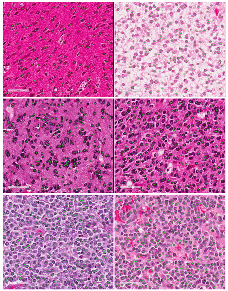
Detection results of several big testing image patches.

For the quantitative comparison, we measure the pixel-wise Euclidean distance between the manually annotated cell centers (ground truth) and the seeds detected by different algorithms. In this assessment, we only consider the correctly detected seeds that are algorithm-produced seeds within 8-pixel distance to the ground truth cell centers. The results are listed in Table II. It can be observed that the proposed method has the smallest variance and a competitive mean error with respect to detection offsets measured by Euclidean distance.

TABLE II.

The comparison of performance evaluated by the Euclidean distance (pixels) from the ground truth cell center to the detected seed. Only the seeds detected within the circular neighborhood of 8-pixel distance around the ground truth cell centers are considered.

Algorithms	Mean	Variance	Min	Max
LoG [22]	3.13	3.14	0	8
IRV [28]	2.85	3.09	0	8
ITCN [54]	3.04	4.02	0	8
SPV [30]	2.7	2.97	0.25	7.9
SR w/o Triv. Templ.	3.06	3.10	0	8
SR w/ Triv. Templ.	2.88	2.64	0	8

To evaluate our algorithm comprehensively, we also define a set of metrics including false negative rate (FN), false positive rate (FP), over-detection rate (OR), effective rate (ER), precision, recall, and F₁ score. FN means no seed is detected within 8-pixel distance to a ground truth seed. FP means for a ground truth seed multiple seeds are detected in its 12-pixel circular neighborhood. OR is the ratio of the number of the overly detected seeds over the number of the ground truth seeds. Ideally, there should be no over detection indicating (i.e., OR = 0). ER is the ratio that will be calculated by the number of the correctly detected seeds over the number of the ground truth seeds (ER = 1 indicates perfect detection). Precision (P), recall (R), and F₁score are defined as $P=\frac{TP}{TP+FP}$, $R=\frac{TP}{TP+FN}$, and $F_1=\frac{2\ast P\ast R}{P+R}$, where TP denotes true positive. In our experiment, true positive is defined as a detected seed that is within 8-pixel distance to a ground truth, and there is no other seeds in a circular region with a radius r = 12 pixels around this ground truth. The comparison results are shown in Table III. It can be observed that the proposed method outperforms all the other methods in terms of all the metrics except for FP and OR, in which ITCN presents the smallest errors. However, this is because ITCN tends to put less detections than the number of cells, which will lead to lower FP and OR, but presenting the highest errors in FP among all the methods.

TABLE III.

The comparison of performance measured by different metrics.

Algorithms	FN	FP	OR	ER	P	R	F1
LoG [22]	0.15	0.004	0.3	0.8	0.94	0.84	0.89
IRV [28]	0.15	0.04	0.07	0.76	0.95	0.83	0.88
ITCN [54]	0.22	0.0005	0.01	0.77	0.99	0.77	0.87
SPV [30]	0.1	0.02	0.06	0.86	0.98	0.89	0.93
SR w/o Triv Templ.	0.09	0.002	0.05	0.91	0.99	0.91	0.95
SR w/ Triv Templ.	0.07	0.0007	0.04	0.92	0.99	0.93	0.96

We also show the precision, recall, and F₁ score as functions of the number of nearest neighbors (10, 25, 50, 75, 100) in the dictionary used in equation (9) for cell detection in Fig. 11(a). The detection accuracy measured by the pixel-wise deviation from the center of the cell (shown in Table II), and different evaluation metrics shown in Table III are illustrated in Fig. 11 (b) and (c), respectively. As we can see, as the number of nearest neighbors increases, the performance improves accordingly. It converges when more than 100 neighbors are selected. The detection result reported in Table II and III are obtained using 100 nearest neighbors in the sparse cell dictionary.

Fig. 11.

Effects of the number of local neighbors in the cell dictionary used in Equation (9) for cell detection. We have experimented with different numbers of nearest neighbors {10, 25, 50, 75, 100}. As the neighbors in the sparse reconstruction increase, the detection results are also improved. (a) Precision, recall, and F₁ score are presented as functions of the number of local neighbors in the sparse dictionary. (b) Mean and variance of the pixel-wise deviation of the seeds generated by the proposed algorithm, and the effective rate (ER) of the detection results. (c) The false negative rate, false positive rate, and the over detection rate of the proposed algorithm.

B. Parameter Selection and Sensitivity

In this subsection we show the effects of parameter selection on the performance. Through experiments, we found that the four parameters, K, m, and γ and z, shown in Table IV are critical to the detection performance. To test the sensitivity of each parameter, we keep other parameters fixed as the optimal value { K = 1400, m = 45 × 45, γ = 10⁻³ } and z is set between 9 and 12 depending on each testing image. In Table IV, for each parameter the first row shows the selection of the values and the second row shows the corresponding F₁ scores. As can be seen that a small parameter K can cause a lower F₁ score due to the limited variation encoded in the dictionary. For patch size m, it is observed that too small and too large patch sizes both can cause drop in performance. This is because the patch size should be large enough to fully contain most cells in the data set. On the contrary, a too large patch contains too much background margin. The reconstruction is then dominated by the error in the margin region. As for γ, a smaller value encourages the trivial templates to contribute more in the reconstruction whereas a larger value restricts the contribution from the trivial templates.

TABLE IV.

Effect of parameter selection on performance.

Parameters	Configurations and the obtained F1 scores
K in Eq.1	250	500	750	1000	1400
	0.92	0.95	0.95	0.958	0.96
patch size m	372	412	452	492	532
	0.92	0.93	0.96	0.93	0.90
γ in Eq.9	10−1	10−2	10−3	10−4	10−5
	0.93	0.944	0.96	0.945	0.95
z in Eq.12	−2	−1	0	1	2
	0.91	0.93	0.96	0.94	0.93

Therefore, larger γ leads to failure in modeling the touching cells. Too small γ enables the model to reconstruct any input images better thus loses the discriminative power. The clustering bandwidth z is determined by the cell size in the testing image. This can be estimated from the radius of the non-touching cells. We show the performance obtained when the clustering bandwidth is less or larger than the best bandwidth by up to 2 pixels. It can be seen that the performance is more sensitive to a smaller bandwidth and less sensitive to larger ones. Other parameters, including λ, N and dictionary size for a testing image are not sensitive. We followed the default setting for λ= 10⁻⁴. The number of the cell pool N controls the richness of the shape variation of the system. A N > 1500 does not affect the performance. Similar to N, sufficient diversity in the testing image specific dictionary is essential for a good performance which requires more than 400 cell patches. We set it to 500 for the experiments.

The parameters of the existing methods under comparison were tuned to the best of their performance. In ITCN, the width and minimum distance are chosen according to the cell size and space between the cells in each testing image [54]. In IRV, the voting diameter is chosen based on the cell size and the threshold are chosen through experiments. For SPV, the most critical parameter is the voting bandwidth d. It is also tuned according to the cell size in each testing image. Other parameters are set as the values suggested in [30] that are {r_min = 0.5d, r_max = 1.5d, Δ = 30, R = (0.3, 0.4, … , 0.9), ${\mathit{bandwidth}}_{MS}=\frac{1}{3}d$}.

C. Computational Complexity

The time complexity mainly consists of three parts: 1) the K-selection, 2) the adaptive dictionary generation, and 3) the sliding window scanning and clustering.

In step one, the K-selection problem is solved by conducting iteratively LLC and basis update via gradient descent. The complexity for LLC in this step is O(K + N), where K denotes the number of the selected bases, and N is the size of the data set. The complexity of one step of the gradient descent is O(KN). The total time complexity is O(T(K + N + KN)), where T is the maximal iterations allowed. This step takes hours on our machine to select 1400 representative bases from the 2000 patches. However, this step is needed for only once at the beginning of the system deployment.

The time complexity of step two depends on the number of representative patches selected in step one and the number of orientations of the sample patch is rotated in the adaptive dictionary generation. Through our experiment we found 1400 representative patches and 5 orientations are sufficient to obtain satisfactory performance. The time cost is about 40 seconds on our machine. This step needs to be done for only once for the images from the same patient.

The time complexity of step three is dominated by the optimization of LLC problem in 9. The optimization of LLC is achieved by using a KNN search and then solving an analytic solution to a least square problem. It does not require an iterative procedure that is computationally expensive. The time complexity is O(k + q + s²), where k denotes the number of nearest neighbors, q represents the dictionary size, and s² is the dimension of the trivial templates that equals to the number of pixels in a sliding window. Given an image of size v×v, the time complexity is O(v²(k+q+s²)). Note that in most cases s ≪ v. The time complexity of the weight guided mean-shift is O(TR²), where T denotes the maximal number of iterations, and R is the number of data points. For an image of size 300×300, the time cost for the sliding window scanning and clustering are about 53 seconds and 2 seconds, respectively. The proposed algorithm is implemented in MATLAB on a machine with Intel 3.4GHz i7 processor and 32GB memory. The space complexity is 120 MB.

IV. Conclusion

In this paper, we have proposed a general, automatic cell detection algorithm using sparse reconstruction with trivial templates and adaptive dictionary learning. By computing the sparse reconstruction with trivial templates, the algorithm is robust and accurate in handling multiple cells (occlusion) in one image patch. The cell appearance variations are tackled by jointly exploiting the testing image specific information and the appearance variations in the learned cell appearance dictionary. The proposed algorithm works well for different images containing cells exhibiting large variations in appearances and shapes. The comparative experiments indicate that our method outperforms other existing state of the arts.

References

- 1.Ferlay J, Soerjomataram I, Ervik M, Dikshit R, Eser S, Mathers C, Rebelo M, Parkin DM, Forman D, Bray F. Globocan 2012 v1.0, cancer incidence and mortality worldwide: Iarc cancerbase no. 11. [07-11-2014]; [Online]. Available: http://globocan.iarc.fr.
- 2.Hu LS, Baxter LC, Smith KA, Feuerstein BG, Karis JP, Eschbacher JM, Coons SW, Nakaji P, Yeh RF, Debbins J, et al. Relative cerebral blood volume values to differentiate high-grade glioma recurrence from posttreatment radiation effect: direct correlation between image-guided tissue histopathology and localized dynamic susceptibility-weighted contrast-enhanced perfusion mr imaging measurements. American Journal of Neuroradiology. 2009;303:552–558. doi: 10.3174/ajnr.A1377. [DOI] [PMC free article] [PubMed] [Google Scholar]
- 3.Lucchinetti CF, Popescu BFG, Bunyan RF, Moll NM, Roemer SF, Lassmann H, Bruck W, Parisi JE, Scheithauer BW, Giannini C, et al. Inflammatory cortical demyelination in early multiple sclerosis. New England Journal of Medicine. 2011;365(23):2188–2197. doi: 10.1056/NEJMoa1100648. [DOI] [PMC free article] [PubMed] [Google Scholar]
- 4.Ghaznavi F, Evans A, Madabhushi A, Feldman M. Digital imaging in pathology: whole-slide imaging and beyond. Annual Review of Pathology: Mechanisms of Disease. 2013;8:331–359. doi: 10.1146/annurev-pathol-011811-120902. [DOI] [PubMed] [Google Scholar]
- 5.Veta M, Pluim JP, van Diest PJ, Viergever MA. Breast cancer histopathology image analysis: A review. IEEE Trans on Biomedical Engineering. 2014 May;61(5):1400–1411. doi: 10.1109/TBME.2014.2303852. [DOI] [PubMed] [Google Scholar]
- 6.Wharton SB, Maltby E, Jellinek DA, Levy D, Atkey N, Hibberd S, Crimmins D, Stoeber K, Williams GH. Subtypes of oligodendroglioma defined by 1p, 19q deletions, differ in the proportion of apoptotic cells but not in replication-licensed non-proliferating cells. Acta neuropathologica. 2007;113(2):119–127. doi: 10.1007/s00401-006-0177-2. [DOI] [PMC free article] [PubMed] [Google Scholar]
- 7.Scheie D, Cvancarova M, Mørk S, Skullerud K, Andresen PA, Benestad I, Helseth E, Meling T, Beiske K. Can morphology predict 1p/19q loss in oligodendroglial tumours? Histopathology. 2008;53(5):578–587. doi: 10.1111/j.1365-2559.2008.03160.x. [DOI] [PubMed] [Google Scholar]
- 8.Malpica N, Ortiz de Solorzano C, Vaquero JJ, Santos A, Vallcorba I, Garcia-Sagredo JM, Pozo Fd. Applying watershed algorithms to the segmentation of clustered nuclei. Journal of Cytometry. 1997;28:289–297. doi: 10.1002/(sici)1097-0320(19970801)28:4<289::aid-cyto3>3.0.co;2-7. [DOI] [PubMed] [Google Scholar]
- 9.Ancin H, Roysam B, Dufresne T, Chestnut M, Ridder G, Szarowski D, Turner J. Advances in automated 3-d image analysis of cell populations imaged by confocal microscopy. Journal of Cytometry. 1996;25(3):22–234. doi: 10.1002/(SICI)1097-0320(19961101)25:3<221::AID-CYTO3>3.0.CO;2-I. [DOI] [PubMed] [Google Scholar]
- 10.Grau V, Mewes AUJ, Alcaniz M, Kikinis R, Warfield S. Improved watershed transform for medical image segmentation using prior information. IEEE Trans on Medical Imaging. 2004;23(4):447–458. doi: 10.1109/TMI.2004.824224. [DOI] [PubMed] [Google Scholar]
- 11.Yang X, Li H, Zhou X. Nuclei segmentation using marker-controlled watershed, tracking using mean-shift, and kalman filter in time-lapse microscopy. IEEE Trans on Circuits and Systems I: Regular Papers. 2006;53(11):2405–2414. [Google Scholar]
- 12.Schmitt O, Hasse M. Radial symmetries based decomposition of cell clusters in binary and gray level images. Journal of Pattern Recognition. 2008 Jun;41(6):1905–1923. [Google Scholar]
- 13.Jung C, Kim C. Segmenting clustered nuclei using h-minima transform-based marker extraction and contour parameterization. IEEE Trans on Biomedical Engineering. 2010 Oct;57(10):2600–2604. doi: 10.1109/TBME.2010.2060336. [DOI] [PubMed] [Google Scholar]
- 14.Cheng J, Rajapakse J. Segmentation of clustered nuclei with shape markers and marking function. IEEE Trans on Biomedical Engineering. 2009 Mar;56(3) doi: 10.1109/TBME.2008.2008635. [DOI] [PubMed] [Google Scholar]
- 15.Mao K, Zhao P, Tan P. Supervised learning-based cell image segmentation for p53 immunohistochemistry. IEEE Trans on Biomedical Engineering. 2006 Jun;53(6):1153–1163. doi: 10.1109/TBME.2006.873538. [DOI] [PubMed] [Google Scholar]
- 16.Yan P, Zhou X, Shah M, Wong S. Automatic segmentation of high-throughput rnai fluorescent cellular images. IEEE Trans on Information Technology in Biomedicine. 2008 Jan;12(1):109–117. doi: 10.1109/TITB.2007.898006. [DOI] [PMC free article] [PubMed] [Google Scholar]
- 17.Lin G, Chawla MK, Olson K, Barnes CA, Guzowski JF, Bjornsson C, Shain W, Roysam B. A multi-model approach to simultaneous segmentation and classification of heterogeneous populations of cell nuclei in 3d confocal microscope images. Cytometry Part A. 2007;71A(9):724–736. doi: 10.1002/cyto.a.20430. [DOI] [PubMed] [Google Scholar]
- 18.Cinar Akakin H, Kong H, Elkins C, Hemminger J, Miller B, Ming J, Plocharczyk E, Roth R, M W, Ziegler R, Lozan-ski G, Gurcan M. Automated detection of cells from immunohistochemically-stained tissues: application to ki-67 nuclei staining. Porc of Medical Imaging 2012: Computer-Aided Diagnosis, SPIE. 2012 Feb;8315 [Google Scholar]
- 19.Kolmogorov V, Zabih R. What energy functions can be minimized via graph cuts? IEEE Trans on Pattern Analysis and Machine Intelligence (TPAMI) 2004;26(2):147–159. doi: 10.1109/TPAMI.2004.1262177. [DOI] [PubMed] [Google Scholar]
- 20.Bernardis E, Yu S. Finding dots: Segmentation as popping out regions from boundaries. Proc of IEEE Conf on Computer Vision and Pattern Recognition (CVPR) 2010 Jun;:199–206. [Google Scholar]
- 21.Shi J, Malik J. Normalized cuts and image segmentation. IEEE Trans on Pattern Analysis and Machine Intelligence (TPAMI) 2000;22(8):888–905. [Google Scholar]
- 22.Al-Kofahi Y, Lassoued W, Lee W, Roysam B. Improved automatic detection and segmentation of cell nuclei in histopathology images. IEEE Trans on Biomedical Engineering. 2010 Apr;57(4):841–852. doi: 10.1109/TBME.2009.2035102. [DOI] [PubMed] [Google Scholar]
- 23.Chang H, Han J, Borowsky A, Loss L, Gray JW, Spell-man PT, Parvin B. Invariant delineation of nuclear architecture in glioblastoma multiforme for clinical and molecular association. IEEE Trans on Medical Imaging. 2013;32(4):670–682. doi: 10.1109/TMI.2012.2231420. [DOI] [PMC free article] [PubMed] [Google Scholar]
- 24.Faustino GM, Gattass M, Rehen S, de Lucena C. Automatic embryonic stem cells detection and counting method in fluorescence microscopy images. Proc of IEEE Inter Symp on Biomedical Imaging: From Nano to Macro (ISBI) 2009:799–802. [Google Scholar]
- 25.Lou X, Koethe U, Wittbrodt J, Hamprecht F. Learning to segment dense cell nuclei with shape prior. Proc of IEEE Conf on Computer Vision and Pattern Recognition (CVPR) 2012 Jun;:1012–1018. [Google Scholar]
- 26.Park C, Huang JZ, Ji JX, Ding Y. Segmentation, inference and classification of partially overlapping nanoparticles. IEEE Trans on Pattern Analysis and Machine Intelligence (TPAMI) 2013;35(3):669–681. doi: 10.1109/TPAMI.2012.163. [DOI] [PubMed] [Google Scholar]
- 27.Cires¸an DC, Giusti A, Gambardella LM, Schmidhuber J. Mitosis detection in breast cancer histology images with deep neural networks. Proc of Medical Image Computing and Computer-Assisted Intervention (MICCAI) 2013:411–418. doi: 10.1007/978-3-642-40763-5_51. [DOI] [PubMed] [Google Scholar]
- 28.Parvin B, Yang Q, Han J, Chang H, Rydberg B, Barcellos-Hoff MH. Iterative voting for inference of structural saliency and characterization of subcellular events. IEEE Trans on Image Processing. 2007;16(3):615–623. doi: 10.1109/tip.2007.891154. [DOI] [PubMed] [Google Scholar]
- 29.Hafiane A, Bunyak F, Palaniappan K. Fuzzy clustering and active contours for histopathology image segmentation and nuclei detection. Proc of Advanced Concepts for Intelligent Vision Systems. 2008:903–914. [Google Scholar]
- 30.Qi X, Xing F, Foran D, Yang L. Robust segmentation of overlapping cells in histopathology specimens using parallel seed detection and repulsive level set. IEEE Trans on Biomedical Engineering. 2012 Mar;59(3):754–765. doi: 10.1109/TBME.2011.2179298. [DOI] [PMC free article] [PubMed] [Google Scholar]
- 31.Kong H, Gurcan M, Belkacem-Boussaid K. Partitioning histopathological images: An integrated framework for supervised color-texture segmentation and cell splitting. IEEE Trans on Medical Imaging. 2011 Sep;30(9):1661–1677. doi: 10.1109/TMI.2011.2141674. [DOI] [PMC free article] [PubMed] [Google Scholar]
- 32.Veta M, van Diest PJ, Kornegoor R, Huisman A, Viergever MA, Pluim JP. Automatic nuclei segmentation in h&e stained breast cancer histopathology images. PloS one. 2013;8(7):e70221. doi: 10.1371/journal.pone.0070221. [DOI] [PMC free article] [PubMed] [Google Scholar]
- 33.Kothari S, Chaudry Q, Wang M. Automated cell counting and cluster segmentation using concavity detection and ellipse fitting techniques. Proc of IEEE Int Symp on Biomedical Imaging (ISBI) 2009 Jul 1;28:795–798. doi: 10.1109/ISBI.2009.5193169. [DOI] [PMC free article] [PubMed] [Google Scholar]
- 34.Su H, Xing F, Lee J, Peterson C, Yang L. Automatic myonuclear detection in isolated single muscle fibers using robust ellipse fitting and sparse optimization. IEEE/ACM Trans on Computational Biology and Bioinformatics. 2013;PP(99):1–1. doi: 10.1109/TCBB.2013.151. [DOI] [PMC free article] [PubMed] [Google Scholar]
- 35.Wright J, Yang AY, Ganesh A, Sastry SS, Ma Y. Robust face recognition via sparse representation. IEEE Trans on Pattern Analysis and Machine Intelligence (TPAMI) 2009;31(2):210–227. doi: 10.1109/TPAMI.2008.79. [DOI] [PubMed] [Google Scholar]
- 36.Liao S, Gao Y, Shen D. Proc of Medical Image Computing and Computer-Assisted Intervention (MICCAI) Springer; 2012. Sparse patch based prostate segmentation in CT images; pp. 385–392. [DOI] [PMC free article] [PubMed] [Google Scholar]
- 37.Zhang S, Li X, Lv J, Jiang X, Zhu D, Chen H, Zhang T, Guo L, Liu T. Proc of Medical Image Computing and Computer-Assisted Intervention (MICCAI) Springer; 2013. Sparse representation of higher-order functional interaction patterns in task-based FMRI data; pp. 626–634. [DOI] [PubMed] [Google Scholar]
- 38.Yu K, Zhang T, Gong Y. Nonlinear learning using local coordinate coding. Proc of Advances in Neural Information Processing Systems (NIPS) 2009;9:1. [Google Scholar]
- 39.Huang Y, Wu Z, Wang L, Tan T. Feature coding in image classification: A comprehensive study. IEEE Trans on Pattern Analysis and Machine Intelligence (TPAMI) 2013 doi: 10.1109/TPAMI.2013.113. [DOI] [PubMed] [Google Scholar]
- 40.Wang J, Yang J, Yu K, Lv F, Huang T, Gong Y. Locality-constrained linear coding for image classification. Proc of IEEE Conf on Computer Vision and Pattern Recognition (CVPR) 2010:3360–3367. [Google Scholar]
- 41.Kårsnäs A, Dahl AL, Larsen R. Learning histopathological patterns. Journal of pathology informatics. 2011;2 doi: 10.4103/2153-3539.92033. [DOI] [PMC free article] [PubMed] [Google Scholar]
- 42.Xing F, Yang L. Robust selection-based sparse shape model for lung cancer image segmentation. Proc of Medical Image Computing and Computer-Assisted Intervention (MICCAI) 2013:404–412. doi: 10.1007/978-3-642-40760-4_51. [DOI] [PMC free article] [PubMed] [Google Scholar]
- 43.Zhou Y, Chang H, Barner K, Spellman P, Parvin B. Classification of histology sections via multispectral convolutional sparse coding. Proc of IEEE Conf on Computer Vision and Pattern Recognition (CVPR) 2014:3081–3088. doi: 10.1109/CVPR.2014.394. [DOI] [PMC free article] [PubMed] [Google Scholar]
- 44.Chang H, Zhou Y, Spellman P, Parvin B. Stacked predictive sparse coding for classification of distinct regions in tumor histopathology. Proc of IEEE Int Conf on Computer Vision (ICCV) 2013:169–176. doi: 10.1109/ICCV.2013.28. [DOI] [PMC free article] [PubMed] [Google Scholar]
- 45.Chang H, Nayak N, Spellman PT, Parvin B. Characterization of tissue histopathology via predictive sparse decomposition and spatial pyramid matching. Medical Image Computing and Computer-Assisted Intervention–MICCAI 2013. 2013:91–98. doi: 10.1007/978-3-642-40763-5_12. [DOI] [PMC free article] [PubMed] [Google Scholar]
- 46.Liu B, Huang J, Yang L, Kulikowsk C. Robust tracking using local sparse appearance model and k-selection. Proc of IEEE Conf on Computer Vision and Pattern Recognition (CVPR) 2011:1313–1320. [Google Scholar]
- 47.Schneider JW, Borlund P. Matrix comparison, part 1: Motivation and important issues for measuring the resemblance between proximity measures or ordination results. Journal of the American Society for Information Science and Technology. 2007;58(11):1586–1595. [Google Scholar]
- 48.Seo HJ, Milanfar P. Training-free, generic object detection using locally adaptive regression kernels. IEEE Trans on Pattern Analysis and Machine Intelligence (TPAMI) 2010;32(9):1688–1704. doi: 10.1109/TPAMI.2009.153. [DOI] [PubMed] [Google Scholar]
- 49.Aharon M, Elad M, Bruckstein A. SVD: An algorithm for designing overcomplete dictionaries for sparse representation. IEEE Trans on Signal Processing. 2006;54(11):4311–4322. [Google Scholar]
- 50.Takeda H, Farsiu S, Milanfar P. Kernel regression for image processing and reconstruction. IEEE Trans on Image Processing (TIP) 2007;16(2):349–366. doi: 10.1109/tip.2006.888330. [DOI] [PubMed] [Google Scholar]
- 51.Comaniciu D, Ramesh V, Meer P. Kernel-based object tracking. IEEE Trans on Pattern Analysis and Machine Intelligence (TPAMI) 2003;25(5):564–577. [Google Scholar]
- 52.Mei X, Ling H. Robust visual tracking using l1 minimization. Proc of IEEE 12th International Conference on Computer Vision; 2009. pp. 1436–1443. [Google Scholar]
- 53.Perona P, Malik J. Scale-space and edge detection using anisotropic diffusion. IEEE Trans on Pattern Analysis and Machine Intelligence (TPAMI) 1990;12(7):629–639. [Google Scholar]
- 54.Byun J, Verardo MR, Sumengen B, Lewis GP, Manjunath B, Fisher SK. Automated tool for the detection of cell nuclei in digital microscopic images: application to retinal images. Mol Vis. 2006;12:949–960. [PubMed] [Google Scholar]