Consistent Cortical Reconstruction and Multi-atlas Brain Segmentation

Abstract

Whole brain segmentation and cortical surface reconstruction are two essential techniques for investigating the human brain. Spatial inconsistences, which can hinder further integrated analyses of brain structure, can result due to these two tasks typically being conducted independently of each other. FreeSurfer obtains self-consistent whole brain segmentations and cortical surfaces. It starts with subcortical segmentation, then carries out cortical surface reconstruction, and ends with cortical segmentation and labeling. However, this “segmentation to surface to parcellation” strategy has shown limitations in various cohorts such as older populations with large ventricles. In this work, we propose a novel “multi-atlas segmentation to surface” method called Multi-atlas CRUISE (MaCRUISE), which achieves self-consistent whole brain segmentations and cortical surfaces by combining multi-atlas segmentation with the cortical reconstruction method CRUISE. A modification called MaCRUISE⁺ is designed to perform well when white matter lesions are present. Comparing to the benchmarks CRUISE and FreeSurfer, the surface accuracy of MaCRUISE and MaCRUISE⁺ is validated using two independent datasets with expertly placed cortical landmarks. A third independent dataset with expertly delineated volumetric labels is employed to compare segmentation performance. Finally, 200 MR volumetric images from an older adult sample are used to assess the robustness of MaCRUISE and FreeSurfer. The advantages of MaCRUISE are: (1) MaCRUISE constructs self-consistent voxelwise segmentations and cortical surfaces, while MaCRUISE⁺ is robust to white matter pathology. (2) MaCRUISE achieves more accurate whole brain segmentations than independently conducting the multi-atlas segmentation. (3) MaCRUISE is comparable in accuracy to FreeSurfer (when FreeSurfer does not exhibit global failures) while achieving greater robustness across an older adult population. MaCRUISE has been made freely available in open source.

Graphical abstract

1. Introduction

Whole brain segmentation and cortical surface reconstruction are two essential automatic techniques for quantitatively investigating MR images (Balafar et al., 2010; Cootes et al., 2001; Lim and Haron, 2014; Pham and Prince, 1999; Van Leemput et al., 1999). Magnetic resonance (MR) images provide morphometric measurements such as region of interest volume (Brewer, 2009; Brewer et al., 2009; Fischl et al., 2002; Keshavan et al., 1995), cortical thickness (Fischl and Dale, 2000; Han et al., 2006; MacDonald et al., 2000), and surface area (Fan et al., 2012; Winkler et al., 2012) using either manual delineation or automatic medical image processing methods (Feczko et al., 2009; Symms et al., 2004). Manual investigation is extremely resource consuming, so validated automatic methods (Cocosco et al., 2003; Van Leemput et al., 1999; Wells et al., 1996) are overwhelmingly preferred.

Atlas-based segmentation assigns tissue labels to the voxels of unlabeled images using a pairing of an anatomical MR image and a corresponding manual segmentation (Cabezas et al., 2011). The pair of images is commonly referred as an atlas. Initially, labels were transferred from a single atlas to a target by image registration (Gass et al., 2013; Guimond et al., 2000; Wu et al., 2007). However, single-atlas segmentation has difficulty capturing large inter-subject anatomical variation (Doan et al., 2010). As reviewed in (Iglesias and Sabuncu, 2015) the de facto standard atlas-based segmentation paradigm, has become to use multiple atlases and carry out label combination (Aljabar et al., 2009; Artaechevarria et al., 2009; Asman et al., 2014; Asman and Landman, 2013; Coupé et al., 2011; Heckemann et al., 2006; Iglesias and Sabuncu, 2015; Isgum et al., 2009; Rohlfing et al., 2004; Sabuncu et al., 2010; Wang et al., 2013; Warfield et al., 2004).

Cortical reconstruction, the localization and representation of human cortical surfaces, is another widely used automatic technique in neuroscience (Dale et al., 1999; Kim et al., 2005; Liu et al., 2008; MacDonald et al., 2000; Shattuck and Leahy, 2002; Xu et al., 1999). Cortical reconstruction has been key to surface based registration (Fischl et al., 1999b; Lyttelton et al., 2007; Tosun and Prince, 2008; Tosun et al., 2004; Yeo et al., 2010), cortical labeling (Desikan et al., 2006; Destrieux et al., 2010; Fischl et al., 2004b), population-based probabilistic atlas generation (Thompson et al., 2001), and surface based morphometry (Chung et al., 2003; Fornito et al., 2008).

Spatial inconsistences that can hinder further brain morphometry analyses might develop because brain segmentation and cortical reconstruction are typically conducted separately. There are limited reports of methods for consistent whole brain volumetric segmentation and cortical surface reconstruction (Fischl, 2012; Han et al., 2004; Stewart et al., 2012). FreeSurfer is a well-known method for whole brain segmentation and cortical reconstruction that has been widely accepted as the de facto standard of brain segmentation (Dale et al., 1999; Fischl, 2012; Fischl et al., 1999a). FreeSurfer first automatically labels whole brain image volumes as gray matter (GM), white matter (WM), cerebrospinal fluid (CSF), and subcortical regions by combining a Markov random field (MRF) and probabilistic atlases into a Bayesian framework (Fischl et al., 2002; Fischl et al., 2004a; Han and Fischl, 2007). Then, an outer (or pial) surface is reconstructed based on the GM/CSF boundaries while an inner surface is reconstructed based on the GM/WM interface (Dale et al., 1999). Finally, the cortical GM regions are labeled based on a surface parcellation that forces the cortical segmentations to be consistent with the surfaces (Desikan et al., 2006; Fischl et al., 2004c). However, since the latter steps strongly rely on the former steps in this “segmentation to surface reconstruction to parcellation” strategy, the cortical parcellation fails when the segmentations and surfaces are reconstructed incorrectly. FreeSurfer has yielded inaccurate whole brain segmentations and cortical surfaces in older adults typically with larger ventricles. When this happens, the resulting surface reconstruction and parcellation are inaccurate.

Cortical surface measurements from FreeSurfer have been evaluated against manual measurements in Alzheimer's disease (Lehmann et al., 2010) and post-mortem histologic measurements (Cardinale et al., 2014). In both cases, FreeSurfer surface estimates showed a high level of correspondence with the manual estimates. Thus, alternative cortical surface algorithms should be consistent with FreeSurfer as long as FreeSurfer operates as intended. Substantial differences would indicate a failure of either FreeSurfer or the novel method. FreeSurfer is not the only approach for segmenting cortical surfaces. Cortical Reconstruction using Implicit Surface Evolution (CRUISE) (Han et al., 2004; Landman et al., 2013; Shiee et al., 2014) is a well-validated method that reconstructs consistent cortical surfaces and fuzzy segmentation (Bazin and Pham, 2007, 2008; Han et al., 2002).

In this paper, we propose a novel “multi-atlas segmentation to surface” method called Multi-atlas Cortical Reconstruction Using Implicit Surface Evolution (MaCRUISE). MaCRUISE simultaneously obtains 133 volumetric labels from a single multi-atlas segmentation and achieves volume consistent and robust cortical surfaces based on the same segmentation. Multi-atlas segmentation is performed with Non-local Spatial Staple (NLSS) (Asman and Landman, 2012, 2013). The main contribution of this work is to integrate cortical reconstruction and multi-atlas segmentation. Specifically: (1) MaCRUISE obtains self-consistent whole brain multi-atlas segmentation (133 labels) and cortical surfaces without compromising surface accuracy. (2) MaCRUISE achieves more accurate volumetric segmentations than a traditional multi-atlas framework. (3) While both deriving consistent whole brain segmentations and cortical surfaces, MaCRUISE is comparable in accuracy to FreeSurfer while achieving greater robustness across an elderly population. Notably, we do not seek to “outperform” FreeSurfer or CRUISE in terms of absolutely accuracy for cases in which these methods work as designed since they have both been extensively validated with respect to human expertise.

This work extends previous conference work (Huo et al., 2016). Herein, we present a more complete description of the MaCRUISE and a more thorough analysis of the performance on an extended dataset. Additionally, we introduce MaCRUISE⁺ (by extending MaCRUISE using the CRUISE⁺ approach (Shiee et al., 2014)) as a method to reconstruct accurate cortical surfaces and volumetric segmentations when multiple sclerosis (MS) lesions are present.

2. Theory and Implementation

MaCRUISE is a method that produces consistent multi-atlas segmentations and cortical reconstruction from T1-weighted MR images (Figure 1). First, cortical surfaces are reconstructed based on estimated tissue class memberships and multi-atlas boundary information. Second, multi-atlas segmentations are refined by the reconstructed cortical surfaces.

Fig. 1.

Block diagram of MaCRUISE. Black text indicates the steps in original CRUISE while red text indicates the additional steps in MaCRUISE.

2.1 Preprocessing

Images are bias corrected with N4 (Tustison et al., 2010) prior to being used as inputs for multi-atlas segmentation (§2.2.1). The bias corrected images are skull stripped with SPECTRE (Carass et al., 2011) and processed by dura stripping (Shiee et al., 2014) in preparation for TOADS (§2.2.2).

2.2 Segmentation

2.2.1 Multi-atlas Segmentation

Multi-atlas segmentation is performed with 45 MPRAGE images from the Open Access Series on Imaging Studies (OASIS) dataset (Marcus et al., 2007). The images are expertly delineated using 133 labels (132 brain regions and 1 background) according to the BrainCOLOR protocol (Klein et al., 2010). All of the 45 OASIS atlases are available from Neuromorphometrics Inc. (http://www.neuromorphometrics.com/) and 35 of the atlases are freely available from the MICCAI 2012 Grand Challenge and Workshop on Multi-Atlas Labeling (Landman and Warfield, 2012) (https://masi.vuse.vanderbilt.edu/workshop2012/).

Briefly, each target image is first affinely registered (Ourselin et al., 2001) to the MNI305 atlas (Evans et al., 1993). Following (Asman et al., 2015; Asman and Landman, 2013), the 15 closest atlases for each target image are selected from the 45 OASIS atlases using PCA projection. The 15 selected atlases are non-rigidly registered to the target image (Avants et al., 2008) and non-local spatial staple label fusion (NLSS) (Asman and Landman, 2012, 2013) is used to combine the labels from each atlas to the target image. For non-rigid registration, we use symmetric image normalization (SyN), with a cross correlation similarity metric convergence threshold of 10⁻⁹ and convergence window size of 15, provided by the Advanced Normalization Tools (ANTs) software (Avants et al., 2008). After multi-atlas labeling, each voxel in the brain is assigned to one of the 133 labels in the BrainCOLOR protocol.

To assist with the cortical reconstruction framework in CRUISE, all cortical GM labels are combined into a single GM segmentation (M_GM). All WM labels and several subcortical labels (nucleus accumbens, amygdala, lateral ventricle, pallidum, putamen, thalamus, and ventral diencephalon) are combined into a single “pseudo-WM” segmentation (M_WM). The “pseudo-WM” subcortical labels are used to define M_WM to mimic the CRUISE “Autofill” procedure (Han et al., 2004). Finally, M_GM, M_WM, and the remaining subcortical labels (hippocampus, amygdala, basal forebrain, and inferior lateral ventricle) are grouped together to form a cerebrum segmentation M_Cerebrum (Figure 2).

Fig. 2.

Results from NLSS multi-atlas segmentation. From the multi-atlas segmentation, we derive cerebrum segmentation (M_Cerebrum), GM segmentation (M_GM) and WM segmentation (M_WM).

2.2.2 Memberships from TOADS

A straightforward way of reconstructing consistent cortical surfaces based on the multi-atlas segmentation is to establish surfaces on NLSS's GM/WM hard segmentation directly (NLSS+CRUISE). However, the atlases are manually labeled based on the expert defined protocol, so objective bias occurs. Moreover, the surface reconstruction suffers from the partial volume effect (PVE) in NLSS's hard segmentation. As shown in Figure 3, independent application of CRUISE after NLSS (NLSS+CRUISE) does not yield accurate surfaces.

Fig. 3.

Here we present the differences and challenges in directly applying multi-atlas hard segmentation to cortical reconstruction. (“NLSS+CRUISE”). (a) shows cortical reconstruction based on GM and WM segmentation using CRUISE. (b) shows the consistent surfaces with NLSS multi-atlas. (c) shows that the outer surface (green) and inner surface (magenta) from NLSS+CRUISE are inaccurate on enlarged 2D overlay (red rectangle). The dotted surfaces indicate the improvements by using the proposed MaCRUISE method (Figure 1).

To address the bias and PVE in multi-atlas segmentation, fuzzy memberships are introduced in MaCRUISE using TOADS (Bazin and Pham, 2008). TOADS conducts fuzzy segmentation on skull and dura stripped T1 volumetric MR images by combining topological and statistical atlases. Finally, robust memberships μ_T of GM, WM, and CSF ( ${{\mu }_T}_{\text{GM}}^i$, ${{\mu }_T}_{\text{WM}}^i$, and ${{\mu }_T}_{\text{CSF}}^i$) for each voxel i are derived from TOADS.

2.2.3 Segmentation Fusion

Multi-atlas hard segmentations are combined with the TOADS memberships to obtain fused GM, WM, and CSF memberships ( ${\mu }_{\text{GM}}^i$, ${\mu }_{\text{WM}}^i$, and ${\mu }_{\text{CSF}}^i$) for each voxel (Figure 4). The combination consists of four stages.

Fig. 4.

Refined segmentations are obtained from segmentation fusion with the following characteristics: (1) PVE issues in NLSS multi-atlas segmentation are resolved (blue rectangles), (2) the fused segmentations have WM labels consistent with TOADS (red rectangles), and (3) non-cerebrum tissues are cleaned by the multi-atlas segmentation (yellow rectangles).

Stage I assigns TOADS membership values within multi-atlas cerebrum segmentations.

$${\mu }_{\text{WM}}^i={{\mu }_T}_{\text{WM}}^i,{\mu }_{\text{GM}}^i={{\mu }_T}_{\text{GM}}^i\text{and}{\mu }_{\text{CSF}}^i={{\mu }_T}_{\text{CSF}}^i\text{if}{M}_{\text{Cerebrum}}^i⩵1$$ (1)

This stage initializes the membership value from the TOADS fuzzy membership function within the multi-atlas cerebrum segmentation M_Cerebrum.

Stage II eliminates all the memberships outside the multi-atlas cerebrum segmentations.

$${\mu }_{\text{WM}}^i=0,{\mu }_{\text{GM}}^i=0\text{and}{\mu }_{\text{CSF}}^i=0\text{if}{M}_{\text{Cerebrum}}^i⩵0$$ (2)

This step not only restricts outer boundaries of brain tissues by cleaning up the remaining dura and skull but also removes the cerebellum and brain stem by multi-atlas segmentations. This replaces the cerebellum and brain stem removal step in TOADS.

Stage III fills in the WM using the multi-atlas WM segmentation, which serves as an approximation of the inner cortical volume.

$${\mu }_{\text{WM}}^i=1,{\mu }_{\text{GM}}^i=0\text{and}{\mu }_{\text{CSF}}^i=0\text{if}{M}_{\text{WM}}^i⩵1$$ (3)

This stage plays a similar role as the “Autofill” procedure in CRUISE, which modifies the WM segmentation by filling the ventricles and subcortical GM structures (e.g., putamen, caudate nucleus, thalamus, hypothalamus).

Stage IV corrects the inaccurate skull-stripping for the voxels whose ${{\mu }_t}_{\text{GM}}^i$ are extremely small — that is, smaller than a constant C within $M_{\text{GM}}^i$. C is empirically set to 0.001 as the default value in MaCRUISE.

$${\mu }_{\text{WM}}^i=0,{\mu }_{\text{GM}}^i=1\text{and}{\mu }_{\text{CSF}}^i=0\text{if}{M}_{\text{GM}}^i⩵1\text{and}{{\mu }_t}_{\text{GM}}^i<C$$ (4)

In other words, if voxel i is labeled as GM in the multi-atlas segmentation but also has an extremely small GM membership value in TOADS, then we trust the multi-atlas segmentation and set the membership value to 1 because this typically happens when skull-stripping fails.

After conducting the previous four stages sequentially, we obtain a fused segmentation that (1) is restricted to multi-atlas cerebrum segmentation, (2) addresses PVE by assigning fuzzy membership values inside the multi-atlas GM hard segmentation, (3) has robust WM filling using multi-atlas WM and subcortical segmentation, and (4) fixes incorrect GM membership values that result from inaccurate skull-stripping.

2.3 Cortical Reconstruction

2.3.1 Multi-atlas Anatomically Consistent GM Enhancement

Although the PVE in GM segmentation is addressed by segmentation fusion, the GM membership function in tight sulci is still obscured or even undetectable because the GM cortex is “back to back” in tight sulcal regions. To detect these sulci, one family of approaches applies cortical thickness constraints to estimate their locations (MacDonald et al., 2000; Zeng et al., 1999). Another approach called Anatomically Consistent Enhancement (ACE) (Han et al., 2004; Han et al., 2001) edits the GM membership values by creating a thin separation between sulcal GM banks based on evidence of the presence of CSF. However, ACE might not be able to detect tight sulci when the presence of CSF is not well captured by TOADS, especially when the contrast between GM and CSF is low. Moreover, the spatial location of sulci from ACE might not be consistent with the multi-atlas segmentation.

To force the estimated sulci to be consistent with multi-atlas segmentation, a hierarchical method called Multi-atlas Anatomically Consistent GM Enhancement (MaACE) is proposed to assign multi-atlas cortical boundaries with the highest priority while estimating the sulci locations (Figure 5). MaACE generalizes ACE for consistency by solving for T(X) in the following Eikonal equation (Han et al., 2004; Sethian, 1999):

Fig. 5.

MaACE compared with the ACE method, (1) MaACE is able to detect sulci in the outer surface that are not detected by ACE, particularly when CSF evidence is not visible (yellow arrow in b). (2) MaACE also forces sulci locations to be consistent with multi-atlas segmentation at the boundaries of cortical labels (red arrow in b). This figure also shows the enhanced GM membership and skeleton from ACE and MaACE (top row).

$$\begin{array}{c}F(\mathrm{X})\parallel \nabla T(\mathrm{X})\parallel =1\text{in}\mathrm{\Omega }\\ T(\mathrm{X})=0\text{for}\mathrm{X}\in \mathrm{\Gamma }\end{array}$$ (5)

where T(X) is the weighted distance function for spatial 3-D position X. F(X) is a speed function (defined below) and Γ is the location of the interface between GM and WM (0.5-isosurface). T(X) can be computed using the fast matching method (Sethian, 1999). If F(X) is equal to one everywhere, then T(X) is the Euclidean distance from the GM/WM interface and the estimated sulci will be located at the midpoint between the gyral banks. The ACE approach defines F(X) to be a spatial varying function that depends on the CSF membership values at x:

$$F(\mathrm{X})=1-0.9{\mu }_{\text{CSF}}(\mathrm{X})$$ (6)

where the μ_CSF(X) is the CSF membership function and the 0.9 is an empirical coefficient. In this case, T(X) can be regarded as the time it takes for a wave front starting from the GM/WM interface to reach x where the speed of the wave front will slow down in the CSF.

Since different cortical labels are separated mainly by sulci location in the BrainCOLOR protocol, cortical boundary locations in the multi-atlas segmentation are used as additional evidence of sulci in MaACE. We combine the boundary information to ACE and specify F(X) as:

$$F(x)=1-0.9(\mathit{max}\{{\mu }_{\text{CSF}}(x),{\mu }_{\text{boundary}}(x)\})$$ (7)

where μ_boundary(x) represents the boundary information in multi-atlas segmentations for which μ_boundary(x) = 1. This is when x is at the “boundary” of cortical labels. The boundary is defined as any cortical voxel that (1) detects two or more different cortical labels among its 26 connections, and (2) does not detect WM labels among its 26 connections.

When using boundary information, MaACE detects additional sulci locations, which are not detected by ACE (yellow arrow in Figure 5b). Meanwhile, MaACE forces the sulci location to be consistent with multi-atlas segmentation (red arrow in Figure 5b). The benefits of Eq. (7), which is a generalized form of Eq. (6), can be understood by considering its action in specific cases:

Case I: F(X) becomes 0.1 when the multi-atlas segmentation boundaries exist with certainty — i.e., μ_boundary(x) = 1. This step forces the estimated sulci to be consistent with the sulci definition in multi-atlas segmentation no matter if CSF evidence exists or not.

Case II: When CSF exists and multi-atlas segmentation boundaries do not (i.e., μ_CSF > μ_boundary(x)), then F(X) becomes formula (6) which is conventional ACE. It forces the estimated sulci to be consistent with the evidence of CSF.

Case III: If we do not have evidence from either multi-atlas boundaries or CSF (i.e., μ_boundary(x) = μ_CSF = 0), then F(X) becomes a constant speed 1 and the sulci are located at the midpoint between sulcal banks (as in conventional ACE).

Using (7) and applying the fast matching method (FMM) starting from the GM/WM interface, segmentation consistent sulci are obtained from the “shocks” — that is, where the wave fronts hit each other (Sethian, 1999). In FMM, new values of T(X) are obtained by solving quadratic equations using F(X) and finite forward and backward difference approximation of ∇T(X) The ACE framework (Han et al., 2004; Han et al., 2001) indicates that if an additional centered finite difference approximation ∇_cT(X) is conducted on the FMM derived T(X), values of F(X)‖∇_cT(X)‖ are much smaller than 1. As a result, the set of shock points are obtained by applying a constant threshold Q.

$$S=\{x|F(\mathrm{X})\parallel {\nabla }_{c}T(\mathrm{X})\parallel \le Q\text{and}T(x)>1\}$$ (8)

The threshold Q is smaller than 1 and empirically set to 0.85. Use of the constraint T(x) > 1 guarantees that the estimated sulci are only found outside the GM/WM surface and at a distance of 1 mm or greater from the GM/WM surface.

The final estimated sulci locations are obtained by conducting a thinning morphological operation on S to obtain its skeleton (which is centered on S and is only one voxel thick). After obtaining this skeleton, the GM membership function is modified as follows.

$${\mu }_{\text{GM}}^{\text{'}}(x)=\{\begin{array}{ll}F(\mathrm{X})\parallel {\nabla }_{c}T(\mathrm{X})\parallel \cdot {\mu }_{\text{GM}}(\mathrm{X})\hfill & \text{if X is on skeleton}\hfill \\ {\mu }_{\text{GM}}(\mathrm{X})\hfill & \text{otherwise}\end{array}$$ (9)

2.3.2 Topology-perserving Deformable Cortical Reconstruction

Three cortical surfaces — inner, central, and outer — are reconstructed with subvoxel accuracy by using the Topology-preserving Geometric Deformable surface Model (TGDM). First, the filled WM membership function is refined by a topology correction step to remove holes and handles. Then, an inner surface is reconstructed using the topological corrected WM membership values (Han et al., 2002; Han et al., 2001). A GVF force (Xu and Prince, 1998), a curvature force, and a regional pressure force are applied to push the inner surface from the GM/WM interface to the pial surface using the TGDM level set approach. The GVF force is generated by the MaACE-corrected GM membership function. The regional pressure force guarantees that the central surface is located within the cortical segmentations. Finally, using the central surface as the initial surface, the outer surface is found using another TGDM step controlled by a curvature force and the MaACE-corrected GM membership function (Han et al., 2004; Osher and Fedkiw, 2006; Osher and Sethian, 1988; Sethian, 1999; Xu et al., 1999). The TGDM method used is the same as that used in the original CRUISE algorithm.

2.4 Cortical Consistent Segmentation Editing

Despite efforts to maintain consistency between the various sources of information, inconsistent voxels still remain at this stage (Figure 6). We introduce the Cortical Consistent Segmentation Editing (CCSE) method to ensure that the multi-atlas segmentation is consistent with the cortical surfaces that have been reconstructed using TGDM. CCSE allows us to define what is “consistent” in a quantitative manner using two coefficients: an inner surface consistency coefficient α and an outer surface consistency coefficient β.

Fig. 6.

The CCSE step corrects the inaccurate cortical labels to background or WM, if they are located outside of the outer surfaces or inside the inner surfaces, respectively. Meanwhile, CCSE adjusts the incorrect volume-wise labels to be cortical labels for voxels between inner and outer surfaces. The distances between voxels and surfaces are provided by the zero set level set functions ϕ_in and ϕ_out. The level of consistency is quantitatively controlled by two consistent coefficients, the inner surface consistent coefficient (α) and the outer surface consistent coefficient (β).

Let ϕ_in and ϕ_out be the level set functions for the inner and outer cortical surfaces reconstructed using TGDM. We can use these functions together with α and β to correct the labels produced by multi-atlas segmentation in the following way: (1) If a voxel is not labeled as background but it is more than β mm outside the outer surface, then we label it as background. (2) If a voxel is more than α mm inside the inner surface but has a background or cortical label that should be outside the GM/WM interface then it is relabeled as WM. (3) In between the outer and inner surfaces, all voxels should be given cortical labels. If a voxel is incorrectly labeled, then it is marked as “needs label” and it is relabeled as one of the 98 cortical labels in the BrainCOLOR protocol using an iterative strategy described in (Plassard et al., 2015). Briefly in each iteration, the remaining “needs label” voxels are filled by the most commonly occurring cortical labels around its 26 connections. This procedure is performed iteratively until all “needs label” voxels are relabeled or no more voxels could be reached. (4) If a voxel is both on skeleton (defined in §2.3.1) and its ϕ_out is 0 ≤ ϕ_out ≤ ε, we keep the original label and the is empirically set to 0.05 mm in MaCRUISE so that the labels with tight “back to back” sulcal surfaces (less than 1 voxel width) are not over corrected.

Although the estimated cortical surfaces have subvoxel accuracy (since they are produced using a connectivity consistent marching cubes algorithm), the multi-atlas segmentation result only has voxel accuracy. This means that distances to the surfaces are reported with subvoxel accuracy but volumetric labels are restricted to the accuracy of the voxels. Since most T1w MR images (obtained for clinical and research purposes) have resolutions on the order of 1mm, it makes sense to choose α and β to be 0.5 mm so that voxels that cover about half of the cortex are given cortical labels. Therefore, both α and β are set to 0.5 mm for the remainder of this manuscript except for in §3.3 where the sensitivity of the algorithm regarding α and β is explored. Note that in the software implementation, users are free to choose alternative values for both α and β.

2.5 Extension to Handle WM Lesions with MaCRUISE⁺

We introduce a variation on MaCRUISE called MaCRUISE⁺, which incorporates the CRUISE⁺ method into the MaCRUISE framework. CRUISE⁺ (Shiee et al., 2014) accurately and automatically reconstructs cortical surfaces when WM lesions are present, which commonly occurs in patients with multiple sclerosis. As with CRUISE⁺, MaCRUISE⁺ uses both Fluid Attenuated Inversion Recovery (FLAIR) T2-weighted (T2w) images and T1w images together with the Lesion-TOADS algorithm (Shiee et al., 2010) in place of the TOADS algorithm. Lesion-TOADS estimates fuzzy membership functions for GM, WM, CSF, and the WM lesions. MaCRUISE⁺ uses the WM mask generated by Lesion-TOADS to remove inaccurate multi-atlas cortical boundaries within the WM lesions. The other steps of MaCRUISE⁺ are identical to those of MaCRUISE.

3. Methods and Results

Validation of the MaCRUISE and MaCRUISE⁺ methods was performed with four distinct datasets and experiments. First (§3.1), absolute surface accuracy of MaCRUISE was compared with the reference methods on a public database of expertly traced cortical surface points for control subjects. Second (§3.2), absolute surface accuracy of MaCRUISE⁺ was compared with the reference methods on a public database of expertly traced cortical surface points for multiple sclerosis patients. Third (§3.3), absolute volumetric accuracy of MaCRUISE was compared with the reference methods on an available (for purchase) database of expertly labeled whole brain volumes. Fourth (§3.4), the robustness of MaCRUISE was assessed relative to the reference methods on a database of older healthy subjects. All validation datasets were obtained from different individuals other than the atlases used to construct the MaCRUISE and MaCRUISE⁺ methods.

3.1 Landmark Based Surface Validation on Healthy Data

3.1.1 Data

The first experiment used a publicly available dataset consisting of five healthy subjects (age range: 30–49) (Landman et al., 2011) with Magnetization Prepared RApid Gradient Echo (MPRAGE) T1-weighted images acquired in the sagittal orientation (resolution=1.0 × 1.0 × 1.2 mm³; FOV=240 × 204 × 256 mm³). In prior work (Shiee et al., 2014), two human raters placed 420 landmarks on both outer and inner surfaces of each subject at the calcarine fissure, cingulate gyrus, central sulcus, parieto-occipital sulcus, superior frontal gyrus, superior temporal gyrus, and Sylvian fissure. The landmarks were made on sulcal fundi, sulcal banks, and gyral crowns with floating point precision. For FreeSurfer, the T1w input images were interpolated to its optimal resolution (1.0 × 1.0 × 1.0 mm³) using the default setting. For CRUISE, the recommended voxel resolution for optimal performance (0.8 × 0.8 × 0.8 mm³) was used.

3.1.3 Experiment and Results

Each of the methods (FreeSurfer, CRUISE, NLSS+CRUISE, and MaCRUISE) was run in an automated manner on each of the 5 datasets. Accuracy was assessed by computing the absolute surface errors (distance from surfaces to landmarks) as shown in Table 1. Briefly, NLSS+CRUISE errors were larger than FreeSurfer and CRUISE, and the surface errors of MaCRUISE were comparable to those of both FreeSurfer and CRUISE. Table 2 statistically evaluates the differences in Table 1 by conducting paired t-tests and Cohen's d effect size (Cohen, 1977) analyses. Note that small p-value might indicate a significant effort of a magnitude that is not clinically relevant, so we rely on both metrics to interpret differences. Figure 7 shows the reconstructed inner and outer surfaces from one subject in the first experiment.

Table 1.

Absolute surface errors on subjects with healthy anatomy with MaCRUISE (mean ± standard deviation in mm).

Optimal resolution*		FreeSurfer	CRUISE	NLSS+CRUISE	MaCRUISE
		1×1×1mm3	0.8×0.8×0.8 mm3	0.8×0.8×0.8 mm3	0.8×0.8×0.8 mm3
Rater A	Outer Surface	0.524 ± 0.372	0.486 ± 0.413	0.880 ± 0.755	0.518 ± 0.414
	Inner Surface	0.460 ± 0.371	0.540 ± 0.429	0.799 ± 0.758	0.544 ± 0.431
Rater B	Outer Surface	0.434 ± 0.369	0.613 ± 0.546	1.050 ± 0.889	0.585 ± 0.464
	Inner Surface	0.432 ± 0.362	0.542 ± 0.483	0.913 ± 0.961	0.544 ± 0.482

^*We resampled the original images to either 1×1×1 mm³ or 0.8×0.8×0.8 mm³ prior to running the different methods. The best results and their corresponding resolutions are reported in this table.

Table 2.

Paired t-test and effect size analyses on absolute surface errors for landmarks with MaCRUISE.

		Rater A		Rater B
		p value	Cohen's d*	p value	Cohen's d
	Outer Surface	<0.001	0.598	<0.001	0.905
	Inner Surface	<0.001	0.567	<0.001	0.662
NLSS+CRUISE vs. CRUISE	Outer Surface	<0.001	0.648	<0.001	0.592
	Inner Surface	<0.001	0.419	<0.001	0.488
	Outer Surface	0.541	0.015	<0.001	0.361
	Inner Surface	<0.001	0.209	<0.001	0.262
	Outer Surface	<0.001	0.078	<0.001	0.055
	Inner Surface	<0.001	0.009	0.145	0.003

^*Cohen's d score is defined as “trivial” (d<0.2), “small effect” (0.2≤d<0.5), “medium effect” (0.5≤d<0.8), or “large effect” (d≥0.8). The bold d value numbers indicate the “medium” or “large” effect. Double underline indicates the significantly superior methods (p<0.001 and d≥0.5), while the dotted underline indicates a lack of evidence for systematic differences (p>0.05 or d<0.5). Single underline indicates the significantly superior methods (p<0.001 and d≥0.5) from at least one rater.

Fig. 7.

Inner and outer surfaces are shown for different methods for a healthy subject. The red and yellow dots in blue and red rectangles are the manual outer and inner surface landmarks, respectively. FreeSurfer and CRUISE are two benchmark methods that achieve accurate surfaces. Note, NLSS+CRUISE does not reconstruct accurate surfaces. Using MaCRUISE, we obtain consistent cortical surfaces and whole brain multi-atlas segmentations. MaCRUISE generates accurate surfaces at lateral ventricles as well as highlighted in yellow rectangles.

3.2 Landmark Based Surface Validation on MaCRUISE⁺

3.2.1 Data

The second experiment used five publicly available MS subjects, consisting of four female subjects and one male subject with a mean age of 48.4 years (range: 40–59) with both MPRAGE and FLAIR images (Shiee et al., 2014). In prior work (Shiee et al., 2014), the images were annotated in both healthy cortical regions and near lesions. The MPRAGE T1w images were acquired in the sagittal orientation with resolution 1.0 × 1.0 × 1.2 mm³. The FLAIR T2w images were acquired in the sagittal orientation but at resolution 0.83 × 0.83 × 2.2 mm³. All datasets were isotropically interpolated to 0.83 × 0.83 × 0.83 mm³ (Shiee et al., 2014). Two human raters labeled 420 landmarks per surface for each MS subject in approximately the same regions of interest (ROI) as described in §3.1 but not near any WM lesions. To evaluate the surface reconstruction performance near WM lesions, five additional ROIs were specified to be near WM lesions. The original two raters and a third human rater each marked 50 landmarks for each MS image. As a result, a total of 2100 landmarks for healthy anatomy and 250 landmarks for cortex near WM lesions were used to evaluate the performance.

3.2.2 Experiment and Results

Each of the methods (FreeSurfer, CRUISE⁺, and MaCRUISE⁺) was run in an automated manner on each of the 5 datasets. As an additional baseline comparison, FreeSurfer was run with the same lesion mask as used by MaCRUISE and MaCRUISE⁺, which was generated by Lesion-TOADS (referred as Corrected FreeSurfer*). Note that since the spatial resolution of the data was already 0.83 mm isotropic to match the highest resolution FLAIR data, all methods used the same data resolution.

Accuracy was assessed by computing the absolute surface errors (distance from surfaces to landmarks) as shown in Table 3 and using paired t-test and effect size analyses as shown in Table 4 with the same approach as in §3.1. The underlined annotations in Table 4 indicate the superior methods (p<0.001 and d≥0.5) (definition found in Table 2). Figure 8 shows the reconstructed inner and outer surfaces from one MS subject with landmarks near WM lesions.

Table 3.

Absolute surface errors with healthy anatomy and WM lesions with MaCRUISE⁺ (mean ± standard deviation in mm).

Landmarks			FreeSurfer	Corrected FreeSurfer*	CRUISE+	MaCRUISE+
Healthy Anatomy	Rater A	Outer Surface	0.445 ± 0.394	0.433 ± 0.339	0.509 ± 0.490	0.529 ± 0.496
		Inner Surface	0.572 ± 0.471	0.511 ± 0.420	0.482 ± 0.455	0.485 ± 0.510
	Rater B	Outer Surface	0.778 ± 1.605	0.600 ± 0.976	0.518 ± 0.539	0.624 ± 0.698
		Inner Surface	0.423 ± 0.326	0.411 ± 0.302	0.368 ± 0.340	0.390 ± 0.354
Near WM Lesions	Rater A	Outer Surface	0.858 ± 1.588	0.679 ± 1.009	0.551 ± 0.566	0.670 ± 0.808
		Inner Surface	0.536 ± 0.488	0.494 ± 0.407	0.337 ± 0.283	0.368 ± 0.293
	Rater B	Outer Surface	0.874 ± 1.498	0.735 ± 1.043	0.589 ± 0.599	0.682 ± 0.755
		Inner Surface	0.476 ± 0.564	0.446 ± 0.551	0.425 ± 0.315	0.387 ± 0.340
	Rater C	Outer Surface	1.028 ± 1.270	0.874 ± 0.878	0.641 ± 0.553	0.705 ± 0.699
		Inner Surface	0.707 ± 0.530	0.696 ± 0.588	0.410 ± 0.293	0.447 ± 0.322

^*FreeSurfer after correction with the WM lesion masks generated by Lesion-TOADS.

Table 4. Paired t-test and effect size analyses on absolute surface errors for landmarks with healthy anatomy and WM lesions with MaCRUISE⁺.

Landmarks			Rater A		Rater B		Rater C
			P value	Cohen's d	P value	Cohen's d	P value	Cohen's d
Healthy Anatomy		Outer Surface	<0.001	0.186	<0.001	0.124
		Inner Surface	<0.001	0.177	<0.001	0.098
		Outer Surface	<0.001	0.226	0.037	0.028
		Inner Surface	<0.001	0.057	0.002	0.065
		Outer Surface	<0.001	0.040	<0.001	0.170
		Inner Surface	0.330	0.006	0.145	0.063
Near WM Lesions	MaCRUISE+ vs.FreeSurfer	Outer Surface	0.022	0.149	0.011	0.162	<0.001	0.315
		Inner Surface	<0.001	0.417	0.024	0.191	<0.001	0.594
	MaCRUISE+ vs. Corrected FreeSurfer*	Outer Surface	0.870	0.010	0.249	0.059	<0.001	0.213
		Inner Surface	<0.001	0.355	0.147	0.128	<0.001	0.526
		Outer Surface	<0.001	0.170	<0.001	0.137	0.003	0.103
		Inner Surface	0.013	0.110	0.005	0.115	0.002	0.121

^*FreeSurfer after correction with the WM lesion masks generated by Lesion-TOADS.

Please see Table 2 for a description of effect size with Cohen's d score.

Fig. 8.

Inner and outer surfaces are shown for each method for an MS subject. Red and yellow dots in blue and red rectangles are the manual outer and inner surface landmarks, respectively, near WM lesions. Based on the landmarks, CRUISE+ and MaCRUISE⁺ achieve more accurate surfaces than FreeSurfer and lesion corrected FreeSurfer*. Note that the corrected FreeSurfer* uses the same lesion mask as CRUISE⁺ and MaCRUISE⁺, which is generated by Lesion-TOADS. From (c), MaCRUISE⁺ achieves consistent cortical surfaces and whole brain segmentations that CRUISE+ does not.

3.3 Segmentation Accuracy

3.3.1 Data

The accuracy of CCSE corrected segmentation was quantitatively evaluated with five MR volumetric images (MPRAGE T1w images with resolution 1.0 × 1.0 × 1.0 mm³) from the OASIS dataset (Marcus et al., 2007). The images were independently labeled by an expert anatomist at Neuromorphometrics Inc. (http://www.neuromorphometrics.com/). The labeling protocols and procedures were the same as with the 45 atlases used in NLSS framework. However, the original 45 atlases have been available and used for several years of algorithm development. We felt that there existed a possibility that the performance could be over-tuned on these datasets, so the five images were retrieved at a later time and were distinct from the original 45 atlases. This approach avoided any unintentional bias that could have been present in a standard cross-validation analysis.

3.3.2 Experiment and Results

Each of the methods (JLF, NLSS, and MaCRUISE with CCSE) was run in an automated manner on each of the 5 datasets. The accuracy of NLSS and CCSE corrected segmentations were evaluated by calculating the Dice values with respect to manual segmentations. To determine statistical differences, we used a Wilcoxon signed rank test on the averaged Dice values (132 labels) for each subject with a sample size n=5 for each test. Moreover, we calculated the averaged Dice values on all cortical labels (98 labels) and WM labels (2 labels). The p value used was 0.05, which is the smallest feasible significance level of n = 5. (Wilcoxon, 1945). We evaluated the sensitivity of MaCRUISE to the consistency coefficients α and β by sweeping them independently from 0 mm to 1 mm with 0.05 mm intervals and re-running all subjects with MaCRUISE for a total of 441 parameter combinations on 5 subjects. As an additional comparison for volumetric accuracy, joint label fusion (JLF) (Wang et al., 2013) was applied to the registered atlases with its default setting on the same data.

MaCRUISE improved segmentations over the entire range of consistency coefficients α and β (Figure 9). The largest improvement averaged over all labels was more than 0.013 Dice (at α = 0.2 mm and β = 0.2 mm). Note that CCSE is based on cortical surfaces, so the largest benefits were seen in cortical labels, while the WM labels were only affected by the inner surface consistency coefficient (α). The lower row of Figure 9 shows a box plot of Dice improvements for α = 0.2 mm, β = 0.2 mm and α = 0.5 mm, β = 0.5 mm. These two sets of coefficients represent those with the largest improvements in this dataset and those that were selected as default values used in MaCRUISE respectively. Both sets of box plots reveal that the Dice values are significantly improved compared to NLSS. Surprisingly, even though the Dice values of WM were already above 0.9, they were improved by nearly 0.03 in the case of α = 0.2 mm and β = 0.2 mm. The use of the default values sacrifices approximately 0.01–0.03 in Dice value over the optimal values. The median Dice values of CCSE were greater than those of JLF, and the CCSE achieved significant better performance than JLF in the case of α = 0.5 mm and β = 0.5 mm.

Fig. 9.

This figure shows the sensitivity MaCRUISE has to α and β by varying them between 0 mm to 1 mm with 0.05 mm intervals. The upper row shows average Dice improvement from NLSS to CSEE in MaCRUISE. (a) The method has maximum improvement when α = 0.2 mm and β = 0.2 mm. (b) The cortical labels follow a similar trend. (c) WM labels are only affected by the inner surface consistent coefficient α. (d) The box plot shows the largest Dice improvements of all 132 labels from this dataset (α = 0.2 mm, β = 0.2 mm) compared to the default values in MaCRUISE (α = 0.5 mm, β = 0.5 mm). (e) and (f) demonstrates the improvements of all 98 cortical labels and 2 WM labels respectively. We compare our approaches with the state-of-the-art JLF method as well. “*” indicates statistically significant difference.

3.4 Robustness of Consistent Cortical Surfaces and Segmentations

3.4.1 Data

We conducted a quantitative and qualitative robustness test on images of 200 control volunteers (100 M/100 F, ages 60.3 to 92.1, mean age 77.6). MPRAGE T1w MR volumetric images were collected as part of the Baltimore Longitudinal Study of Aging (BLSA) study, which is a study of aging operated by the National Institute on Aging (Resnick et al., 2003; Shock et al., 1984).

3.4.2 Experiment and Results

Each of the methods (FreeSurfer, CRUISE, and MaCRUISE) was run in an automated manner on each of the 200 datasets. Average surface distance (ASD) and correlation analyses were conducted to evaluate the global performance and consistency between MaCRUISE and the benchmarks (CRUISE and FreeSurfer). The number of global failures (outliers) was used as the robustness metric. First, the surface distance (Han et al., 2006) between MaCRUISE and the benchmarks was examined to detect outliers. The artificial surface regions that separate the two hemispheres in FreeSurfer were excluded from the ASD measurement since MaCRUISE and CRUISE do not have such surfaces. Second, the segmentations of the lateral ventricles were examined to identify additional failures.

Mean ASD between MaCRUISE and the benchmark algorithms are generally around or smaller than 0.5 mm (Figure 10a). However, there are four images (marked using red numbers 1 through 4) that are located outside of a margin of 2.5 standard deviations. These large surface distances indicate that at least one of the methods failed with these images. For the ventricle volumes, a strong linear correlation was found except in seven outlier volumes (marked using green numbers 4 through 11) (Figure 10b). Thus, a total of 11 failed volumes were automatically detected. The segmentations and surfaces of the failures for these subjects are shown in Figure 11 (red outliers) and Figure 12 (green outliers). The global failures (in the red rectangles) occur in all 11 volumes for FreeSurfer and in two volumes for CRUISE. In contrast, we do not find any global failures from MaCRUISE. Therefore, none of the 11 failures are attributable to MaCRUISE. To complete the analysis, we visually inspected the surfaces and segmentations for the remaining 189 volumes and did not find any global failures for either MaCRUISE or the benchmark algorithms.

Fig. 10.

This figure shows the average surface distance (ASD) between different methods and the correlation of lateral ventricle size for the population of elderly subjects. (a) The ASD between MaCRUISE with CRUISE and FreeSurfer is less than 0.5 mm in most cases, but four outliers are found. (b) The size of lateral ventricle is plotted using FreeSurfer and MaCRUISE which identified seven more outliers. A total of 11 inconsistent outliers are detected where failures occured in one of the methods. We note that FreeSurfer systematically estimates smaller ventricle size than MaCRUISE in the outliers.

Fig. 11.

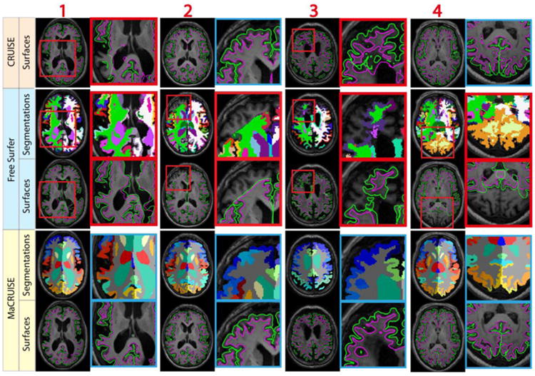
The four outliers from surface distance analysis are shown. Both whole brain segmentations and cortical surfaces on axial slices are provided. The areas in red rectangles show the global failures in FreeSurfer whereas MaCRUISE did not exhibit any such failures.

Fig. 12.

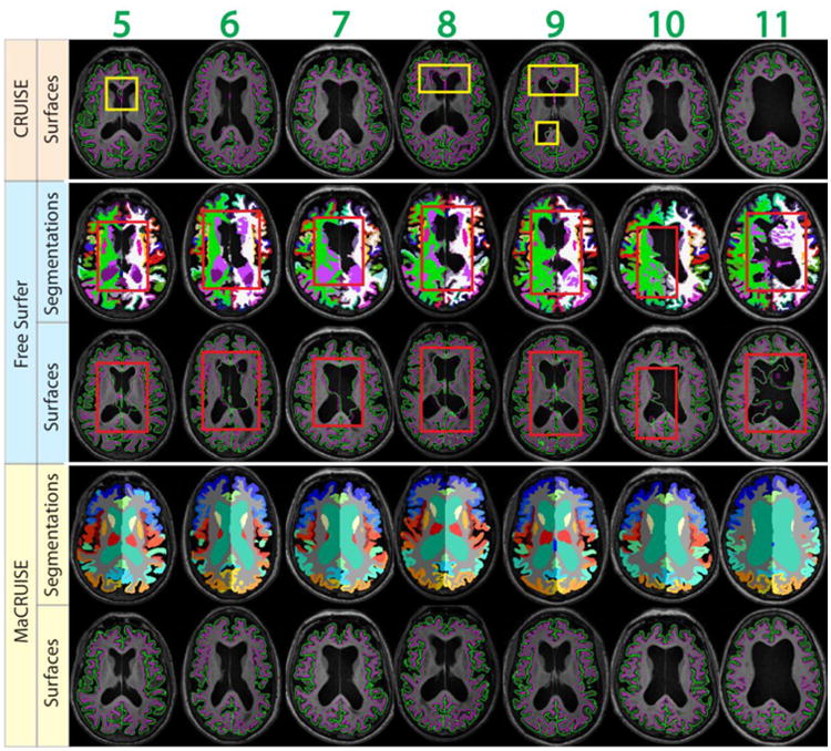
The seven outliers from inconsistent lateral ventricle size are shown. Both whole brain segmentations and cortical surfaces on axial slices are provided. The areas in red rectangles show the global failures while the areas in yellow rectangles show the local inaccurate surfaces. MaCRUISE did not exhibit such failures in any images.

Discussion

MaCRUISE is an open framework that allows users to replace NLSS and TOADS with other multi-atlas or fuzzy segmentation approaches. MaCRUISE⁺ is an example of replacing TOADS with Lesion-TOADS (also available as open source), which incorporates the MaCRUISE framework in the case of pathology. MaCRUISE and MaCRUISE⁺ are publicly available as open source software through the JIST software package (http://www.nitrc.org/projects/jist/) (Li et al., 2012; Lucas et al., 2010). MaCRUISE is also implemented as a plugin called “PlugInsMaCRUISE” in CRUISE software. The source code is available using CVS access (www.nitrc.org:/cvsroot/toads-cruise).

While FreeSurfer has been widely used and is regarded as the de facto standard method for generating whole brain segmentations and cortical surface locations. FreeSurfer failed globally in about 5% of older adult populations from a BLSA sample dataset. Even though manual correction would probably address these failures, the time required for manual correction makes it undesirable. Compared with FreeSurfer, the proposed MaCRUISE achieves (1) greater robustness in older populations, and (2) comparable accuracy on normal healthy images (§3.1). To the best of our knowledge, this is the first work that integrates multi-atlas segmentation into cortical reconstruction. Moreover, the perspective of using multi-atlas segmentation and the proposed consistency adjustment approaches could be integrated into FreeSurfer, which might improve the robustness of FreeSurfer on older adult populations. The statistical analyses using both paired t-test and effect size analyses indicate a lack of evidence for systematic differences (p>0.05 or d<0.5) between MaCRUISE and CRUISE when examining datasets on which CRUISE has been validated. Therefore, the proposed MaCRUISE achieves comparably accurate cortical surfaces compared with the CRUISE method while providing consistent whole brain segmentation when the original CRUISE method does not.

Consistency is another essential challenge in clinical and scientific analyses of MR brain images. MaCRUISE establishes consistent brain segmentation and cortical surfaces by combining multi-atlas segmentation with cortical reconstruction. However, the naive strategy of directly deploying CRUISE after NLSS (NLSS+CRUISE) did not yield accurate surfaces. With the specific contributions of this work (i.e., segmentation fusion, MaACE, and CCSE), MaCRUISE improves both surface (Tables 1-4) and volumetric accuracy (Figure 9).

While MaCRUISE shows great promise for consistent multi-atlas segmentation and cortical reconstruction, there are certain areas that warrant further investigation. We used NLSS framework as the multi-atlas segmentation algorithm and employed TOADS as the fuzzy segmentation approach. Since the two different segmentation methods are conducted independently, inconsistency exists between their segmentations. To reconcile the inconsistency, the segmentation fusion method (§2.2.3) is used in the MaCRUISE. While this is highly successful, we do not claim optimality of using NLSS and TOADS. Using other multi-atlas or fuzzy segmentation methods might yield a better performance when establishing consistent multi-atlas segmentation and cortical reconstruction. Since the proposed method is an open framework, users are encouraged to explore methods other than NLSS and TOADS freely. Recently, (Tustison et al., 2014) indicated that the Advanced Normalization Tools (ANTs) based framework achieved a higher predictive performance than FreeSurfer by evaluating thickness-based prediction of age and gender. Such analyses of predictive power are relevant, but depend heavily on the population context. For example, a method that exaggerated aging effects would have greater power to detect aging, but could be less accurate in an absolute sense and potentially less useful when aging is not an effect of interest. Examining predictive power of MaCRUISE versus other approaches would be a valuable direction for further investigation.

There are potential drawbacks in the presented MaCRUISE approach. First, the robustness of multi-atlas segmentation framework comes at the cost of computational complexity from both expensive non-rigid registration and non-local correspondences calculations. Empirically, MaCRUISE typically takes approximately 38 hours. This is broken up into NLSS framework (≈36 h), TOADS segmentations (≈1 h) and cortical reconstruction (≈1 h) on a single core of an Intel Xeon W3550 4 Core CPU (64 bit Ubuntu Linux 14.04). As a result, MaCRUISE has much greater time complexity than CRUISE (<2h) or FreeSurfer (<15 h) on the same machine. Recently, a learning based multi-atlas framework called multi-atlas learner fusion (MLF) has been proposed to reduce the time that multi-atlas segmentation requires to less than 10 minutes (Asman et al., 2015). Replacing the NLSS by MLF would be a promising way of reducing the total computing time of MaCRUISE to less than 3 hours. Second, both the multi-atlas segmentation and TOADS results are functions of the imaging sequence and are thus biased based on the sequence (Plassard et al., 2016). Contrast synthesis may become an important approach to ensure performance across imaging sequences e.g., following (Jog et al., 2015). Third, the cortical surfaces derived between subjects do not have pre-defined correspondence, which necessitates surface and/or image registration. Finally, we do not claim the optimality of the number of atlases used in the experiments. Fifteen atlases were chosen based on our previous experience with the collection of 45 available atlases (Asman et al., 2015; Asman and Landman, 2013). Users may wish to optimize the number of atlases for their application via cross-validation or bootstrapping (Iglesias and Sabuncu, 2015).

Conclusion

Herein, we introduced MaCRUISE, a novel consistent whole brain segmentation and cortical surface reconstruction approach using multi-atlas segmentation. MaCRUISE achieved greater robustness on T1w MRI images from older adults than FreeSurfer without compromising on the accuracy of normal healthy images. MaCRUISE achieves significantly greater volumetric accuracy than solely using NLSS multi-atlas segmentation. MaCRUISE⁺ established consistent cortical surfaces and volumetric segmentations for images with WM lesions.

From landmark based surface validation, we demonstrated that MaCRUISE achieved consistent whole brain multi-atlas segmentation and cortical reconstruction (Figure 7) without compromising accuracy (Table 1 and 2) since the differences between MaCRUISE and the benchmark algorithms are either “trivial” (d<0.2) or “small effect” (d<0.5). MaCRUISE⁺ was similarly accurate (Table 3 and 4) and provided consistent whole brain segmentations (Figure 8). MaCRUISE allows users to control the consistency level between whole brain segmentations and reconstructed surfaces using the consistency coefficients α and β. The refined segmentations achieved robust improvements on a wide range of different α's and β's (0 mm to 1 mm) compared to NLSS (Figure 9). Finally, by evaluation of gross failures on a collection of 200 volumetric images from older adults, MaCRUISE is more robust to errors in surface segmentation than CRUISE or FreeSurfer (Figure 10, 11 and 12). In all cases, MaCRUISE achieved consistent segmentations of the cortical surface and all brain labels, which was not the case for either CRUISE or FreeSurfer.

Highlights.

• A novel approach called MaCRUISE is introduced, which establishes consistent multi-atlas segmentation and cortical reconstruction using a single MRI T1w image.

• MaCRUISE is comparable in accuracy to CRUISE and FreeSurfer, while achieving greater robustness across an older adult population.

• More accurate in whole brain segmentations than independently conducting the NLSS multiatlas segmentation framework.

• The method has been made freely available in open source.

References

- Aljabar P, Heckemann RA, Hammers A, Hajnal JV, Rueckert D. Multi-atlas based segmentation of brain images: atlas selection and its effect on accuracy. Neuroimage. 2009;46:726–738. doi: 10.1016/j.neuroimage.2009.02.018. [DOI] [PubMed] [Google Scholar]
- Artaechevarria X, Munoz-Barrutia A, Ortiz-de-Solorzano C. Combination strategies in multi-atlas image segmentation: application to brain MR data. IEEE Trans Med Imaging. 2009;28:1266–1277. doi: 10.1109/TMI.2009.2014372. [DOI] [PubMed] [Google Scholar]
- Asman AJ, Dagley AS, Landman BA. Statistical label fusion with hierarchical performance models. Proc Soc Photo Opt Instrum Eng. 2014;9034:90341E. doi: 10.1117/12.2043182. [DOI] [PMC free article] [PubMed] [Google Scholar]
- Asman AJ, Huo Y, Plassard AJ, Landman BA. Multi-atlas learner fusion: An efficient segmentation approach for large-scale data. Med Image Anal. 2015;26:82–91. doi: 10.1016/j.media.2015.08.010. [DOI] [PMC free article] [PubMed] [Google Scholar]
- Asman AJ, Landman BA. Formulating spatially varying performance in the statistical fusion framework. IEEE Trans Med Imaging. 2012;31:1326–1336. doi: 10.1109/TMI.2012.2190992. [DOI] [PMC free article] [PubMed] [Google Scholar]
- Asman AJ, Landman BA. Non-local statistical label fusion for multi-atlas segmentation. Med Image Anal. 2013;17:194–208. doi: 10.1016/j.media.2012.10.002. [DOI] [PMC free article] [PubMed] [Google Scholar]
- Avants BB, Epstein CL, Grossman M, Gee JC. Symmetric diffeomorphic image registration with cross-correlation: evaluating automated labeling of elderly and neurodegenerative brain. Med Image Anal. 2008;12:26–41. doi: 10.1016/j.media.2007.06.004. [DOI] [PMC free article] [PubMed] [Google Scholar]
- Balafar MA, Ramli AR, Saripan MI, Mashohor S. Review of brain MRI image segmentation methods. Artificial Intelligence Review. 2010;33:261–274. [Google Scholar]
- Bazin PL, Pham DL. Topology-preserving tissue classification of magnetic resonance brain images. IEEE Trans Med Imaging. 2007;26:487–496. doi: 10.1109/TMI.2007.893283. [DOI] [PubMed] [Google Scholar]
- Bazin PL, Pham DL. Homeomorphic brain image segmentation with topological and statistical atlases. Med Image Anal. 2008;12:616–625. doi: 10.1016/j.media.2008.06.008. [DOI] [PMC free article] [PubMed] [Google Scholar]
- Brewer JB. Fully-automated volumetric MRI with normative ranges: translation to clinical practice. Behav Neurol. 2009;21:21–28. doi: 10.3233/BEN-2009-0226. [DOI] [PMC free article] [PubMed] [Google Scholar]
- Brewer JB, Magda S, Airriess C, Smith ME. Fully-automated quantification of regional brain volumes for improved detection of focal atrophy in Alzheimer disease. AJNR Am J Neuroradiol. 2009;30:578–580. doi: 10.3174/ajnr.A1402. [DOI] [PMC free article] [PubMed] [Google Scholar]
- Cabezas M, Oliver A, Llado X, Freixenet J, Cuadra MB. A review of atlas-based segmentation for magnetic resonance brain images. Comput Methods Programs Biomed. 2011;104:e158–177. doi: 10.1016/j.cmpb.2011.07.015. [DOI] [PubMed] [Google Scholar]
- Carass A, Cuzzocreo J, Wheeler MB, Bazin PL, Resnick SM, Prince JL. Simple paradigm for extra-cerebral tissue removal: algorithm and analysis. Neuroimage. 2011;56:1982–1992. doi: 10.1016/j.neuroimage.2011.03.045. [DOI] [PMC free article] [PubMed] [Google Scholar]
- Cardinale F, Chinnici G, Bramerio M, Mai R, Sartori I, Cossu M, Russo GL, Castana L, Colombo N, Caborni C. Validation of FreeSurfer-estimated brain cortical thickness: comparison with histologic measurements. Neuroinformatics. 2014;12:535–542. doi: 10.1007/s12021-014-9229-2. [DOI] [PubMed] [Google Scholar]
- Chung MK, Worsley KJ, Robbins S, Paus T, Taylor J, Giedd JN, Rapoport JL, Evans AC. Deformation-based surface morphometry applied to gray matter deformation. Neuroimage. 2003;18:198–213. doi: 10.1016/s1053-8119(02)00017-4. [DOI] [PubMed] [Google Scholar]
- Cocosco CA, Zijdenbos AP, Evans AC. A fully automatic and robust brain MRI tissue classification method. Med Image Anal. 2003;7:513–527. doi: 10.1016/s1361-8415(03)00037-9. [DOI] [PubMed] [Google Scholar]
- Cohen J. Statistical power analysis for the behavioral sciences. Lawrence Erlbaum Associates, Inc; 1977. [Google Scholar]
- Cootes TF, Edwards GJ, Taylor CJ. Active appearance models. Ieee Transactions on Pattern Analysis and Machine Intelligence. 2001;23:681–685. [Google Scholar]
- Coupé P, Manjón JV, Fonov V, Pruessner J, Robles M, Collins DL. Patch-based segmentation using expert priors: Application to hippocampus and ventricle segmentation. Neuroimage. 2011;54:940–954. doi: 10.1016/j.neuroimage.2010.09.018. [DOI] [PubMed] [Google Scholar]
- Dale AM, Fischl B, Sereno MI. Cortical surface-based analysis. I. Segmentation and surface reconstruction. Neuroimage. 1999;9:179–194. doi: 10.1006/nimg.1998.0395. [DOI] [PubMed] [Google Scholar]
- Desikan RS, Segonne F, Fischl B, Quinn BT, Dickerson BC, Blacker D, Buckner RL, Dale AM, Maguire RP, Hyman BT, Albert MS, Killiany RJ. An automated labeling system for subdividing the human cerebral cortex on MRI scans into gyral based regions of interest. Neuroimage. 2006;31:968–980. doi: 10.1016/j.neuroimage.2006.01.021. [DOI] [PubMed] [Google Scholar]
- Destrieux C, Fischl B, Dale A, Halgren E. Automatic parcellation of human cortical gyri and sulci using standard anatomical nomenclature. Neuroimage. 2010;53:1–15. doi: 10.1016/j.neuroimage.2010.06.010. [DOI] [PMC free article] [PubMed] [Google Scholar]
- Doan NT, de Xivry JO, Macq B. SPIE Medical Imaging International Society for Optics and Photonics. 2010. Effect of inter-subject variation on the accuracy of atlas-based segmentation applied to human brain structures; pp. 76231S-76231S–76210. [Google Scholar]
- Evans AC, Collins DL, Mills S, Brown E, Kelly R, Peters TM. 1993 IEEE Conference Record. IEEE; 1993. 3D statistical neuroanatomical models from 305 MRI volumes. Nuclear Science Symposium and Medical Imaging Conference, 1993; pp. 1813–1817. [Google Scholar]
- Fan SW, Zhou ZJ, Hu ZJ, Fang XQ, Zhao FD, Zhang J. Quantitative MRI analysis of the surface area, signal intensity and MRI index of the central bright area for the evaluation of early adjacent disc degeneration after lumbar fusion. Eur Spine J. 2012;21:1709–1715. doi: 10.1007/s00586-012-2293-0. [DOI] [PMC free article] [PubMed] [Google Scholar]
- Feczko E, Augustinack JC, Fischl B, Dickerson BC. An MRI-based method for measuring volume, thickness and surface area of entorhinal, perirhinal, and posterior parahippocampal cortex. Neurobiology of Aging. 2009;30:420–431. doi: 10.1016/j.neurobiolaging.2007.07.023. [DOI] [PMC free article] [PubMed] [Google Scholar]
- Fischl B. FreeSurfer. Neuroimage. 2012;62:774–781. doi: 10.1016/j.neuroimage.2012.01.021. [DOI] [PMC free article] [PubMed] [Google Scholar]
- Fischl B, Dale AM. Measuring the thickness of the human cerebral cortex from magnetic resonance images. Proc Natl Acad Sci U S A. 2000;97:11050–11055. doi: 10.1073/pnas.200033797. [DOI] [PMC free article] [PubMed] [Google Scholar]
- Fischl B, Salat DH, Busa E, Albert M, Dieterich M, Haselgrove C, van der Kouwe A, Killiany R, Kennedy D, Klaveness S, Montillo A, Makris N, Rosen B, Dale AM. Whole brain segmentation: automated labeling of neuroanatomical structures in the human brain. Neuron. 2002;33:341–355. doi: 10.1016/s0896-6273(02)00569-x. [DOI] [PubMed] [Google Scholar]
- Fischl B, Salat DH, van der Kouwe AJ, Makris N, Segonne F, Quinn BT, Dale AM. Sequence-independent segmentation of magnetic resonance images. Neuroimage. 2004a;23 Suppl 1:S69–84. doi: 10.1016/j.neuroimage.2004.07.016. [DOI] [PubMed] [Google Scholar]
- Fischl B, Sereno MI, Dale AM. Cortical surface-based analysis. II: Inflation, flattening, and a surface-based coordinate system. Neuroimage. 1999a;9:195–207. doi: 10.1006/nimg.1998.0396. [DOI] [PubMed] [Google Scholar]
- Fischl B, Sereno MI, Tootell RBH, Dale AM. High-resolution intersubject averaging and a coordinate system for the cortical surface. Human brain mapping. 1999b;8:272–284. doi: 10.1002/(SICI)1097-0193(1999)8:4<272::AID-HBM10>3.0.CO;2-4. [DOI] [PMC free article] [PubMed] [Google Scholar]
- Fischl B, van der Kouwe A, Destrieux C, Halgren E, Segonne F, Salat DH, Busa E, Seidman LJ, Goldstein J, Kennedy D, Caviness V, Makris N, Rosen B, Dale AM. Automatically parcellating the human cerebral cortex. Cerebral Cortex. 2004b;14:11–22. doi: 10.1093/cercor/bhg087. [DOI] [PubMed] [Google Scholar]
- Fischl B, van der Kouwe A, Destrieux C, Halgren E, Segonne F, Salat DH, Busa E, Seidman LJ, Goldstein J, Kennedy D, Caviness V, Makris N, Rosen B, Dale AM. Automatically parcellating the human cerebral cortex. Cereb Cortex. 2004c;14:11–22. doi: 10.1093/cercor/bhg087. [DOI] [PubMed] [Google Scholar]
- Fornito A, Yucel M, Wood SJ, Adamson C, Velakoulis D, Saling MM, McGorry PD, Panteliss C. Surface-based morphometry of the anterior cingulate cortex in first episode schizophrenia. Human brain mapping. 2008;29:478–489. doi: 10.1002/hbm.20412. [DOI] [PMC free article] [PubMed] [Google Scholar]
- Gass T, Székely G, Goksel O. Medical Computer Vision Recognition Techniques and Applications in Medical Imaging. Springer; 2013. Semi-supervised segmentation using multiple segmentation hypotheses from a single atlas; pp. 29–37. [Google Scholar]
- Guimond A, Meunier J, Thirion JP. Average brain models: A convergence study. Computer Vision and Image Understanding. 2000;77:192–210. [Google Scholar]
- Han X, Fischl B. Atlas renormalization for improved brain MR image segmentation across scanner platforms. IEEE Trans Med Imaging. 2007;26:479–486. doi: 10.1109/TMI.2007.893282. [DOI] [PubMed] [Google Scholar]
- Han X, Jovicich J, Salat D, van der Kouwe A, Quinn B, Czanner S, Busa E, Pacheco J, Albert M, Killiany R, Maguire P, Rosas D, Makris N, Dale A, Dickerson B, Fischl B. Reliability of MRI-derived measurements of human cerebral cortical thickness: the effects of field strength, scanner upgrade and manufacturer. Neuroimage. 2006;32:180–194. doi: 10.1016/j.neuroimage.2006.02.051. [DOI] [PubMed] [Google Scholar]
- Han X, Pham DL, Tosun D, Rettmann ME, Xu C, Prince JL. CRUISE: cortical reconstruction using implicit surface evolution. Neuroimage. 2004;23:997–1012. doi: 10.1016/j.neuroimage.2004.06.043. [DOI] [PubMed] [Google Scholar]
- Han X, Xu C, Braga-Neto U, Prince JL. Topology correction in brain cortex segmentation using a multiscale, graph-based algorithm. IEEE Trans Med Imaging. 2002;21:109–121. doi: 10.1109/42.993130. [DOI] [PubMed] [Google Scholar]
- Han X, Xu C, Tosun D, Prince JL. Mathematical Methods in Biomedical Image Analysis, 2001 MMBIA 2001 IEEE Workshop on. IEEE; 2001. Cortical surface reconstruction using a topology preserving geometric deformable model; pp. 213–220. [Google Scholar]
- Heckemann RA, Hajnal JV, Aljabar P, Rueckert D, Hammers A. Automatic anatomical brain MRI segmentation combining label propagation and decision fusion. Neuroimage. 2006;33:115–126. doi: 10.1016/j.neuroimage.2006.05.061. [DOI] [PubMed] [Google Scholar]
- Huo Y, Carass A, Resnick SM, Pham DL, Prince JL, Landman BA. SPIE Medical Imaging International Society for Optics and Photonics. 2016. Combining multi-atlas segmentation with brain surface estimation; pp. 97840E-97840E–97848. [DOI] [PMC free article] [PubMed] [Google Scholar]
- Iglesias JE, Sabuncu MR. Multi-atlas segmentation of biomedical images: A survey. Med Image Anal. 2015;24:205–219. doi: 10.1016/j.media.2015.06.012. [DOI] [PMC free article] [PubMed] [Google Scholar]
- Isgum I, Staring M, Rutten A, Prokop M, Viergever MA, van Ginneken B. Multi-atlas-based segmentation with local decision fusion--application to cardiac and aortic segmentation in CT scans. IEEE Trans Med Imaging. 2009;28:1000–1010. doi: 10.1109/TMI.2008.2011480. [DOI] [PubMed] [Google Scholar]
- Jog A, Carass A, Roy S, Pham DL, Prince JL. MR image synthesis by contrast learning on neighborhood ensembles. Medical image analysis. 2015;24:63–76. doi: 10.1016/j.media.2015.05.002. [DOI] [PMC free article] [PubMed] [Google Scholar]
- Keshavan MS, Anderson S, Beckwith C, Nash K, Pettegrew JW, Krishnan KR. A comparison of stereology and segmentation techniques for volumetric measurements of lateral ventricles in magnetic resonance imaging. Psychiatry Res. 1995;61:53–60. doi: 10.1016/0925-4927(95)02446-5. [DOI] [PubMed] [Google Scholar]
- Kim JS, Singh V, Lee JK, Lerch J, Ad-Dab'bagh Y, MacDonald D, Lee JM, Kim SI, Evans AC. Automated 3-D extraction and evaluation of the inner and outer cortical surfaces using a Laplacian map and partial volume effect classification. Neuroimage. 2005;27:210–221. doi: 10.1016/j.neuroimage.2005.03.036. [DOI] [PubMed] [Google Scholar]
- Klein A, Dal Canton T, Ghosh SS, Landman B, Lee J, Worth A. Open labels: online feedback for a public resource of manually labeled brain images. 16th Annual Meeting for the Organization of Human Brain Mapping 2010 [Google Scholar]
- Landman B, Warfield S. MICCAI 2012 workshop on multi-atlas labeling. Medical Image Computing and Computer Assisted Intervention Conference 2012: MICCAI 2012 Grand Challenge and Workshop on Multi-Atlas Labeling Challenge Results 2012 [Google Scholar]
- Landman BA, Bogovic JA, Carass A, Chen M, Roy S, Shiee N, Yang Z, Kishore B, Pham D, Bazin PL, Resnick SM, Prince JL. System for integrated neuroimaging analysis and processing of structure. Neuroinformatics. 2013;11:91–103. doi: 10.1007/s12021-012-9159-9. [DOI] [PMC free article] [PubMed] [Google Scholar]
- Landman BA, Huang AJ, Gifford A, Vikram DS, Lim IA, Farrell JA, Bogovic JA, Hua J, Chen M, Jarso S, Smith SA, Joel S, Mori S, Pekar JJ, Barker PB, Prince JL, van Zijl PC. Multi-parametric neuroimaging reproducibility: a 3-T resource study. Neuroimage. 2011;54:2854–2866. doi: 10.1016/j.neuroimage.2010.11.047. [DOI] [PMC free article] [PubMed] [Google Scholar]
- Lehmann M, Douiri A, Kim LG, Modat M, Chan D, Ourselin S, Barnes J, Fox NC. Atrophy patterns in Alzheimer's disease and semantic dementia: a comparison of FreeSurfer and manual volumetric measurements. Neuroimage. 2010;49:2264–2274. doi: 10.1016/j.neuroimage.2009.10.056. [DOI] [PubMed] [Google Scholar]
- Li B, Bryan F, Landman BA. Next Generation of the Java Image Science Toolkit (JIST): Visualization and Validation. Insight J. 2012;2012:1–16. [PMC free article] [PubMed] [Google Scholar]
- Lim SP, Haron H. Surface reconstruction techniques: a review. Artificial Intelligence Review. 2014;42:59–78. [Google Scholar]
- Liu T, Nie J, Tarokh A, Guo L, Wong ST. Reconstruction of central cortical surface from brain MRI images: method and application. Neuroimage. 2008;40:991–1002. doi: 10.1016/j.neuroimage.2007.12.027. [DOI] [PMC free article] [PubMed] [Google Scholar]
- Lucas BC, Bogovic JA, Carass A, Bazin PL, Prince JL, Pham DL, Landman BA. The Java Image Science Toolkit (JIST) for rapid prototyping and publishing of neuroimaging software. Neuroinformatics. 2010;8:5–17. doi: 10.1007/s12021-009-9061-2. [DOI] [PMC free article] [PubMed] [Google Scholar]
- Lyttelton O, Boucher M, Robbins S, Evans A. An unbiased iterative group registration template for cortical surface analysis. Neuroimage. 2007;34:1535–1544. doi: 10.1016/j.neuroimage.2006.10.041. [DOI] [PubMed] [Google Scholar]
- MacDonald D, Kabani N, Avis D, Evans AC. Automated 3-D extraction of inner and outer surfaces of cerebral cortex from MRI. Neuroimage. 2000;12:340–356. doi: 10.1006/nimg.1999.0534. [DOI] [PubMed] [Google Scholar]
- Marcus DS, Wang TH, Parker J, Csernansky JG, Morris JC, Buckner RL. Open Access Series of Imaging Studies (OASIS): cross-sectional MRI data in young, middle aged, nondemented, and demented older adults. J Cogn Neurosci. 2007;19:1498–1507. doi: 10.1162/jocn.2007.19.9.1498. [DOI] [PubMed] [Google Scholar]
- Osher S, Fedkiw R. Level set methods and dynamic implicit surfaces. Springer Science & Business Media; 2006. [Google Scholar]
- Osher S, Sethian JA. Fronts propagating with curvature-dependent speed: algorithms based on Hamilton-Jacobi formulations. Journal of Computational Physics. 1988;79:12–49. [Google Scholar]
- Ourselin S, Roche A, Subsol G, Pennec X, Ayache N. Reconstructing a 3D structure from serial histological sections. Image and Vision Computing. 2001;19:25–31. [Google Scholar]
- Pham DL, Prince JL. Adaptive fuzzy segmentation of magnetic resonance images. IEEE Trans Med Imaging. 1999;18:737–752. doi: 10.1109/42.802752. [DOI] [PubMed] [Google Scholar]
- Plassard AJ, Harrigan RL, Newton AT, Rane S, Pallavaram S, D'Haese PF, Dawant BM, Claassen DO, Landman BA. SPIE Medical Imaging International Society for Optics and Photonics. 2016. On the fallacy of quantitative segmentation for T1-weighted MRI; pp. 978416-978416–978417. [DOI] [PMC free article] [PubMed] [Google Scholar]
- Plassard AJ, Hinton KE, Venkatraman V, Gonzalez C, Resnick SM, Landman BA. Evaluation of Atlas-Based White Matter Segmentation with Eve. Proc SPIE Int Soc Opt Eng. 2015;9413 doi: 10.1117/12.2081613. [DOI] [PMC free article] [PubMed] [Google Scholar]
- Resnick SM, Pham DL, Kraut MA, Zonderman AB, Davatzikos C. Longitudinal magnetic resonance imaging studies of older adults: a shrinking brain. J Neurosci. 2003;23:3295–3301. doi: 10.1523/JNEUROSCI.23-08-03295.2003. [DOI] [PMC free article] [PubMed] [Google Scholar]
- Rohlfing T, Russakoff DB, Maurer CR., Jr Performance-based classifier combination in atlas-based image segmentation using expectation-maximization parameter estimation. IEEE Trans Med Imaging. 2004;23:983–994. doi: 10.1109/TMI.2004.830803. [DOI] [PubMed] [Google Scholar]
- Sabuncu MR, Yeo BT, Van Leemput K, Fischl B, Golland P. A generative model for image segmentation based on label fusion. IEEE Trans Med Imaging. 2010;29:1714–1729. doi: 10.1109/TMI.2010.2050897. [DOI] [PMC free article] [PubMed] [Google Scholar]
- Sethian JA. Level set methods and fast marching methods: evolving interfaces in computational geometry, fluid mechanics, computer vision, and materials science. Cambridge university press; 1999. [Google Scholar]
- Shattuck DW, Leahy RM. BrainSuite: an automated cortical surface identification tool. Med Image Anal. 2002;6:129–142. doi: 10.1016/s1361-8415(02)00054-3. [DOI] [PubMed] [Google Scholar]
- Shiee N, Bazin PL, Cuzzocreo JL, Ye C, Kishore B, Carass A, Calabresi PA, Reich DS, Prince JL, Pham DL. Reconstruction of the human cerebral cortex robust to white matter lesions: method and validation. Human brain mapping. 2014;35:3385–3401. doi: 10.1002/hbm.22409. [DOI] [PMC free article] [PubMed] [Google Scholar]
- Shiee N, Bazin PL, Ozturk A, Reich DS, Calabresi PA, Pham DL. A topology-preserving approach to the segmentation of brain images with multiple sclerosis lesions. Neuroimage. 2010;49:1524–1535. doi: 10.1016/j.neuroimage.2009.09.005. [DOI] [PMC free article] [PubMed] [Google Scholar]
- Shock NW, Greulich RC, Andres R, Arenberg D, Costa PT, Lakatta EG, Tobin JD. NIH Publication, No 84-2450. 1984. Normal human aging: The Baltimore longitudinal study of aging. [Google Scholar]
- Stewart JC, Zielke DJ, Hawkins MA, Williams DR, Carnethon MR, Knox SS, Matthews KA. Depressive symptom clusters and 5-year incidence of coronary artery calcification: the coronary artery risk development in young adults study. Circulation. 2012;126:410–417. doi: 10.1161/CIRCULATIONAHA.112.094946. [DOI] [PMC free article] [PubMed] [Google Scholar]
- Symms M, Jager HR, Schmierer K, Yousry TA. A review of structural magnetic resonance neuroimaging. J Neurol Neurosurg Psychiatry. 2004;75:1235–1244. doi: 10.1136/jnnp.2003.032714. [DOI] [PMC free article] [PubMed] [Google Scholar]
- Thompson PM, Mega MS, Woods RP, Zoumalan CI, Lindshield CJ, Blanton RE, Moussai J, Holmes CJ, Cummings JL, Toga AW. Cortical change in Alzheimer's disease detected with a disease-specific population-based brain atlas. Cerebral Cortex. 2001;11:1–16. doi: 10.1093/cercor/11.1.1. [DOI] [PubMed] [Google Scholar]
- Tosun D, Prince JL. A Geometry-Driven Optical Flow Warping for Spatial Normalization of Cortical Surfaces. IEEE Trans Med Imaging. 2008;27:1739–1753. doi: 10.1109/TMI.2008.925080. [DOI] [PMC free article] [PubMed] [Google Scholar]
- Tosun D, Rettmann ME, Prince JL. Mapping techniques for aligning sulci across multiple brains. Med Image Anal. 2004;8:295–309. doi: 10.1016/j.media.2004.06.020. [DOI] [PMC free article] [PubMed] [Google Scholar]
- Tustison NJ, Avants BB, Cook PA, Zheng Y, Egan A, Yushkevich PA, Gee JC. N4ITK: improved N3 bias correction. IEEE Trans Med Imaging. 2010;29:1310–1320. doi: 10.1109/TMI.2010.2046908. [DOI] [PMC free article] [PubMed] [Google Scholar]
- Tustison NJ, Cook PA, Klein A, Song G, Das SR, Duda JT, Kandel BM, van Strien N, Stone JR, Gee JC, Avants BB. Large-scale evaluation of ANTs and FreeSurfer cortical thickness measurements. Neuroimage. 2014;99:166–179. doi: 10.1016/j.neuroimage.2014.05.044. [DOI] [PubMed] [Google Scholar]
- Van Leemput K, Maes F, Vandermeulen D, Suetens P. Automated model-based tissue classification of MR images of the brain. IEEE Trans Med Imaging. 1999;18:897–908. doi: 10.1109/42.811270. [DOI] [PubMed] [Google Scholar]
- Wang HZ, Suh JW, Das SR, Pluta JB, Craige C, Yushkevich PA. Multi-Atlas Segmentation with Joint Label Fusion. Ieee Transactions on Pattern Analysis and Machine Intelligence. 2013;35:611–623. doi: 10.1109/TPAMI.2012.143. [DOI] [PMC free article] [PubMed] [Google Scholar]
- Warfield SK, Zou KH, Wells WM. Simultaneous truth and performance level estimation (STAPLE): an algorithm for the validation of image segmentation. IEEE Trans Med Imaging. 2004;23:903–921. doi: 10.1109/TMI.2004.828354. [DOI] [PMC free article] [PubMed] [Google Scholar]
- Wells WM, Grimson WL, Kikinis R, Jolesz FA. Adaptive segmentation of MRI data. IEEE Trans Med Imaging. 1996;15:429–442. doi: 10.1109/42.511747. [DOI] [PubMed] [Google Scholar]
- Wilcoxon F. Individual comparisons by ranking methods. Biometrics bulletin. 1945:80–83. [Google Scholar]
- Winkler AM, Sabuncu MR, Yeo BT, Fischl B, Greve DN, Kochunov P, Nichols TE, Blangero J, Glahn DC. Measuring and comparing brain cortical surface area and other areal quantities. Neuroimage. 2012;61:1428–1443. doi: 10.1016/j.neuroimage.2012.03.026. [DOI] [PMC free article] [PubMed] [Google Scholar]
- Wu M, Rosano C, Lopez-Garcia P, Carter CS, Aizenstein HJ. Optimum template selection for atlas-based segmentation. Neuroimage. 2007;34:1612–1618. doi: 10.1016/j.neuroimage.2006.07.050. [DOI] [PubMed] [Google Scholar]
- Xu C, Pham DL, Rettmann ME, Yu DN, Prince JL. Reconstruction of the human cerebral cortex from magnetic resonance images. IEEE Trans Med Imaging. 1999;18:467–480. doi: 10.1109/42.781013. [DOI] [PubMed] [Google Scholar]
- Xu C, Prince JL. Snakes, shapes, and gradient vector flow. IEEE Trans Image Process. 1998;7:359–369. doi: 10.1109/83.661186. [DOI] [PubMed] [Google Scholar]
- Yeo BTT, Sabuncu MR, Vercauteren T, Ayache N, Fischl B, Golland P. Spherical Demons: Fast Diffeomorphic Landmark-Free Surface Registration. IEEE Trans Med Imaging. 2010;29:650–668. doi: 10.1109/TMI.2009.2030797. [DOI] [PMC free article] [PubMed] [Google Scholar]
- Zeng X, Staib LH, Schultz RT, Duncan JS. Segmentation and measurement of the cortex from 3-D MR images using coupled-surfaces propagation. IEEE Trans Med Imaging. 1999;18:927–937. doi: 10.1109/42.811276. [DOI] [PubMed] [Google Scholar]