Measurement of a vacuum-induced geometric phase

A Berry phase is induced on an artificial atom coupled to a quantum field in the vacuum state by slowly varying their coupling.

Abstract

Berry’s geometric phase naturally appears when a quantum system is driven by an external field whose parameters are slowly and cyclically changed. A variation in the coupling between the system and the external field can also give rise to a geometric phase, even when the field is in the vacuum state or any other Fock state. We demonstrate the appearance of a vacuum-induced Berry phase in an artificial atom, a superconducting transmon, interacting with a single mode of a microwave cavity. As we vary the phase of the interaction, the artificial atom acquires a geometric phase determined by the path traced out in the combined Hilbert space of the atom and the quantum field. Our ability to control this phase opens new possibilities for the geometric manipulation of atom-cavity systems also in the context of quantum information processing.

INTRODUCTION

Geometric phases are at the heart of many phenomena in solid-state physics (1), from the quantum Hall effect (2) to topological phases (3, 4), and may provide a resource for quantum computation (5, 6). As a quantum system is steered in its state space by controlled interaction with an external field, the trajectory it describes can be associated with a geometric phase (7). Although the external field is typically treated as classical, its quantization is expected to produce novel geometric effects at low excitation numbers (8). Here, we experimentally demonstrate that a geometric phase of Berry’s type (7) can be induced by a variable coupling between the system and a quantized field, using a superconducting circuit. This phase is nonvanishing even when the quantized field is in the vacuum state, a result with no semiclassical analog. It has been referred to as the vacuum-induced Berry phase (8), and its existence and observability have been the subject of theoretical debate (8–11). According to Larson (10), it is an artifact of the rotating-wave approximation. However, later work by Wang et al. (11) shows that a vacuum-induced Berry phase is always associated with the Rabi model, regardless of whether the rotating-wave approximation is used. No evidence of this phase has been observed thus far, possibly due to the difficulty in engineering the relevant interaction, whereas superconducting circuits have already been used to study geometric phases (12–16), their susceptibility to noise (17), and their relation to topological effects (18, 19).

In previous measurements of the Berry phase (13, 20), a transition between two quantum states |g〉 and |f〉 was driven by a coherent field of amplitude α, detuning Δ, and phase ϕ (Fig. 1A). In a frame rotating at the drive frequency, the corresponding dynamics is that of a spin-½ particle interacting with an effective magnetic field $\overrightarrow{\mathit{B}}$ = (2gα cosϕ, 2gα sinϕ, Δ), where g is the dipole strength of the transition. An adiabatic variation of ϕ causes $\overrightarrow{\mathit{B}}$ to precess around the ẑ axis; the corresponding path traced out by the spin particle in its Hilbert space can be obtained by projecting the vector $\overrightarrow{\mathit{B}}$ onto the Bloch sphere (Fig. 1B). The spin particle, initially in its ground state, acquires a geometric phase γ = Ω/2, where Ω is the solid angle subtended by the circular path (7).

Fig. 1. Berry phase induced by a quantized field.

(A) An atomic transition between two states, |g〉 and |f〉, is driven by a coherent tone of amplitude α, phase ϕ, and detuning Δ. The phase ϕ is slowly varied between 0 and 2π. (B) In a frame rotating at the drive frequency, the drive acts as an effective magnetic field (red thick arrow) precessing around the ẑ axis. In the adiabatic limit, the Bloch vector stays aligned with the field and describes a circular path on the Bloch sphere spanned by the atomic basis states |g〉 and |f〉. The acquired geometric phase equals half the solid angle Ω subtended by the path. (C) By placing the atom in a cavity, the atom interacts with a quantized field. The interaction between the atom and the field is controlled by a microwave-activated coupling, which is mediated by an intermediate state |e〉 and is tunable in amplitude g and phase ϕ. (D) Admissible paths on the Bloch sphere for different numbers of photons n in the cavity. For each n, the Bloch sphere is spanned by the basis states |g, n + 1〉 and |f, n〉 of the combined atom-cavity system.

As noticed by Fuentes-Guridi et al. (8), the model presented in Fig. 1A is a semiclassical one: It ignores the quantization of the applied field and neglects the effect of vacuum fluctuations on the Berry phase. By contrast, a fully quantized version of the problem is captured by the Hamiltonian

$$\widehat{\mathit{H}}=\frac{\mathrm{\Delta }}{2}{\widehat{\mathrm{\sigma }}}_{\mathit{z}}+\mathit{g}({\widehat{\mathrm{\sigma }}}_{+}\widehat{\mathit{a}}{\mathit{e}}^{-\mathit{i}\mathrm{\varphi }}+{\widehat{\mathrm{\sigma }}}_{-}{\widehat{\mathit{a}}}^{†}{\mathit{e}}^{\mathit{i}\mathrm{\varphi }})$$ (1)

where ${\widehat{\mathrm{\sigma }}}_{\mathit{z}}$ is a Pauli matrix acting on the Hilbert space {|g〉, |f〉} of the two-level system, Δ is the detuning of the quantized field, g is the coupling, and â, â^†, ${\widehat{\mathrm{\sigma }}}_{-}$, and ${\widehat{\mathrm{\sigma }}}_{+}$ are the annihilation and creation operators of the quantized field and the two-level system, respectively. This Hamiltonian describes a Jaynes-Cummings–type interaction with a variable phase ϕ and gives rise to a finite Berry phase also in the limit of vanishing photon number (8).

In our experiment, we realize a tunable coupling between a cavity mode and two levels, |g〉 and |f〉, of a superconducting artificial atom, by applying a coherent microwave signal (21–24), as schematically shown in Fig. 1C and detailed in the following. A slow modulation of the coupling phase realizes a geometric manipulation, which is the quantum analog of the semiclassical evolution depicted in Fig. 1 (A and B). To understand its effects, consider the eigenstates of the Hamiltonian (Eq. 1). The ground state |g, 0〉 is not coupled to any other state; as such, it acquires no geometric phase. The other eigenstates are coupled in pairs $|{\mathrm{\Psi }}_{\mathit{n}}^{\pm }\rangle$ having support in the subspaces {|f, n〉, |g, n + 1〉}, with n denoting the photon number in the cavity. As ϕ is adiabatically steered, each subspace undergoes a different evolution, shown in Fig. 1D for the first few photon numbers. The geometric phase accumulated by the states $|{\mathrm{\Psi }}_{\mathit{n}}^{\pm }\rangle$ is given by (8)

$${\mathrm{\gamma }}_{\mathit{n}}^{\pm }=\mathrm{\pi }[1\mp \frac{\mathrm{\Delta }}{\sqrt{{\mathrm{\Delta }}^2+4{\mathit{g}}^2(\mathit{n}+1)}}]$$ (2)

A comparison to Fig. 1B highlights two key features of the quantized model: (i) for a given coupling g and detuning Δ, only a discrete set of paths are admissible, corresponding to integer values of n, and (ii) a finite solid angle is enclosed even when n = 0, corresponding to a vacuum-induced Berry phase.

RESULTS

Experimental setup

Our setup consists of a transmon-type superconducting circuit embedded in a three-dimensional (3D) microwave cavity (16, 25). The distribution of the electric field for the first two modes of the cavity is shown in Fig. 2B. The position of the coupling ports is such that the first mode is overcoupled, whereas the second mode is strongly undercoupled. We use the ground state and the second excited state of the transmon (|g〉 and |f〉, respectively) as the two atomic states and the second mode of the cavity as the quantized field. A diagram of all relevant frequencies for our experiment is shown in Fig. 2C. To read out the ground state and the first and second excited states of the transmon, we measured the state-dependent transmission through the fundamental mode (26). By applying a control field close to the nominal frequency ω_d = ω_ge + ω_ef − ω₂, we induce a microwave-activated coupling between pairs of states |f, n〉 and |g, n + 1〉, with amplitude ge^iϕ and detuning Δ (23, 24) (see the Supplementary Materials for details).

Fig. 2. Transmon in a 3D cavity with mode-selective coupling ports.

(A) Edited photograph of the 3D cavity used in the experiment. Two sapphire chips are placed inside the cavity. A transmon is patterned on the left chip (blue circle). (B) Cross section of the electric field magnitude |$\overrightarrow{\mathit{E}}$| for the two lowest-frequency modes of the cavity in (A), as obtained from a finite-element simulation. The chip used in the experiment is highlighted in blue, and the cavity ports are indicated as circles (not drawn to scale). (C) Diagram of the relevant frequencies for the experiment: first three cavity modes, ω₁, ω₂, and ω₃ (red), first two transitions of the transmon, ω_ge and ω_ef (blue), and higher-order transition between states |f0〉 and |g1〉, ω_d (yellow).

Resonant vacuum-induced Berry phase

We first report on measurements performed in the resonant case Δ = 0, and with the cavity initially in the vacuum state n = 0. Our scheme for measuring the geometric phase (Fig. 3A) relies on the use of |e〉 as a reference state for Ramsey interferometry. The measured thermal population of |e〉 is about 1% and is neglected in our analysis. Starting from the ground state |g, 0〉, we first prepare the superposition state $\frac{1}{\sqrt{2}}(|\mathit{f}0\rangle +|\mathit{e}0\rangle )$ and then apply a resonant coupling pulse to bring the state |f0〉 into $|{\mathrm{\Psi }}_0^{-}\rangle =\frac{1}{\sqrt{2}}(|\mathit{g}1\rangle +|\mathit{f}0\rangle )$. At this point, we again turn on the coupling, choosing its phase so that the effective magnetic field is aligned with the prepared eigenstate $|{\mathrm{\Psi }}_0^{-}\rangle$ (see also the Supplementary Materials). Then, we slowly vary the phase by an amount δϕ = 2π. A third coupling pulse follows to bring the system back to |f0〉. The phase carried by |f0〉, which includes a geometric contribution from the phase manipulation, is finally detected by Ramsey interferometry against the reference state |e0〉, using a final π/2 pulse on the |e〉 ↔ |f〉 transition with variable phase ϕ_R. To single out the geometric contribution to the interference phase, we compare patterns obtained with (δϕ = 2π) and without (δϕ = 0) the phase variation because the acquired dynamic phase (including Stark shifts) is the same in both cases. The recorded interference patterns clearly oscillate out of phase (Fig. 3B), with a measured phase shift ${\mathrm{\gamma }}_0^{-}$ = (3.13 ± 0.06). This result can be explained by a geometric argument: when Δ = 0, the Bloch vector describes a loop on the equator (compare Fig. 1D). The enclosed solid angle is Ω = 2π, corresponding to a geometric phase π. We have repeated this measurement for different durations τ of the middle coupling pulse. As we keep δϕ = 2π, this results in the same geometric loop being traced out at different speeds. For each measurement, we extract the phase ${\mathrm{\gamma }}_0^{-}$ from the shift between the two Ramsey patterns and plot it versus τ (Fig. 3C, circles). The data are clustered around the value π, confirming that ${\mathrm{\gamma }}_0^{-}$ is largely independent of the rate at which we sweep ϕ, as long as the evolution stays adiabatic. This is a strong indication of the geometric character of ${\mathrm{\gamma }}_0^{-}$. For the fastest pulses considered, we see systematic deviations from the value π. This behavior must be expected as the speed is increased, due to the breakdown of the adiabatic assumption. In the present case, the adiabaticity parameter can be written as A = π/(gτ) = 0.52 μs/τ. The crossover between adiabatic and nonadiabatic dynamics is expected when A ≈ 1 and τ ≈ 0.5 μs, in agreement with the data of Fig. 3C.

Fig. 3. Vacuum-induced Berry phase: Resonant case.

(A) Pulse sequence to detect the geometric phase acquired by the state $|{\mathrm{\Psi }}_{\mathit{n}}^{-}\rangle$ for resonant coupling (Δ = 0). The cavity is prepared in an n-photon Fock state by repeating the initial sequence n times. The system is prepared in a superposition of |e, n〉 and $|{\mathrm{\Psi }}_{\mathit{n}}^{-}\rangle$. Then, the resonant coupling is turned on, and its phase is increased by 2π during a time τ. Finally, the relative phase between $|{\mathrm{\Psi }}_{\mathit{n}}^{-}\rangle$ and |e, n〉 is determined by Ramsey interferometry. (B) Oscillations observed in the e-state population P_e when varying the phase ϕ_R of the second Ramsey pulse, with τ = 420 ns and n = 0. The measurement described in (A) (δϕ = 2π; dark magenta squares) is compared against a reference measurement in which the phase of the coupling is held fixed (δϕ = 0; blue circles). The phase shift observed in the Ramsey pattern corresponds to an accumulated geometric phase ${\mathrm{\gamma }}_0^{-}$ = (3.13 ± 0.06). (C) Geometric phase γ, determined as in (B), versus pulse duration τ. Three different states are prepared: the two eigenstates, $|{\mathrm{\Psi }}_0^{-}\rangle$ (blue circles) and $|{\mathrm{\Psi }}_0^{+}\rangle$ (dark magenta squares), and the state |f0〉 (yellow diamonds), for which the cavity is initially in the vacuum state. (D) Geometric phase accumulated by the states $|{\mathrm{\Psi }}_{\mathit{n}}^{\pm }\rangle$ and |f, n〉, with fixed pulse duration τ and varying photon number n.

Using the same technique, we measure the phase acquired by the other eigenstate $|{\mathrm{\Psi }}_0^{+}\rangle$. By adding a phase shift of π to the coupling pulse, we turn $|{\mathrm{\Psi }}_0^{-}\rangle$ into $|{\mathrm{\Psi }}_0^{+}\rangle$ because the pseudospin is now aligned opposite to the effective magnetic field. The resulting geometric phase ${\mathrm{\gamma }}_0^{+}$ (Fig. 3C, squares) follows a similar trend as ${\mathrm{\gamma }}_0^{-}$, approaching π in the adiabatic limit and deviating at shorter pulse durations. In addition, we consider the state |f0〉, for which the field mode is initially in the vacuum state. To prepare and measure |f0〉, we omit the first and third coupling pulses. Because |f0〉 is not an eigenstate of Eq. 1, we select only those pulse durations τ = πk/g, with an integer k, that give rise to a cyclic evolution. The resulting series (Fig. 3C, diamonds), in agreement with the other two, provides direct evidence of the vacuum-induced Berry phase. Finally, we prepare an n-photon Fock state in the cavity and measure the phases acquired by the states $|{\mathrm{\Psi }}_{\mathit{n}}^{\pm }\rangle$ and |f, n〉 (Fig. 3D). The mean geometric phase, averaged over different states and different photon numbers n = 0,…,4, is 〈γ〉 = (3.1 ± 0.2) ≈ π. We thus conclude that, at resonance, the Berry phase is essentially independent of the photon number in the cavity.

Berry phase at finite detuning

In contrast to the resonant case, a photon number–dependent geometric phase is to be expected at finite detuning Δ between the atom and the field because in that case, the enclosed solid angle depends on the ratio $\mathrm{\Delta }/(\mathit{g}\sqrt{\mathit{n}+1})$ (Fig. 1D). Furthermore, according to Eq. 2, the two eigenstates $|{\mathrm{\Psi }}_{\mathit{n}}^{-}\rangle$ and $|{\mathrm{\Psi }}_{\mathit{n}}^{+}\rangle$ acquire different phases: ${\mathrm{\gamma }}_{\mathit{n}}^{-}\ne {\mathrm{\gamma }}_{\mathit{n}}^{+}$ for Δ ≠ 0. To measure the relative geometric phase between $|{\mathrm{\Psi }}_{\mathit{n}}^{-}\rangle$ and $|{\mathrm{\Psi }}_{\mathit{n}}^{+}\rangle$ at arbitrary detuning, we use the pulse sequence described in Fig. 4A. First of all, we notice that for a generic Δ, the state |f, n〉 = α(Δ)$|{\mathrm{\Psi }}_{\mathit{n}}^{-}\rangle$ + β(Δ)$|{\mathrm{\Psi }}_{\mathit{n}}^{+}\rangle$ is a superposition of $|{\mathrm{\Psi }}_{\mathit{n}}^{\pm }\rangle$; as such, |f, n〉 can be directly used for Ramsey interferometry. The coefficients α(Δ) and β(Δ) determine the visibility of the interference pattern. Because a measurement based on |f, n〉 only involves the two states $|{\mathrm{\Psi }}_{\mathit{n}}^{\pm }\rangle$, it allows us to use a spin-echo technique to cancel out the dynamic phase. Although a spin echo is typically implemented by applying an inverting π pulse, here we prefer to engineer the effective Hamiltonian (Eq. 1) so that the states $|{\mathrm{\Psi }}_{\mathit{n}}^{\pm }\rangle$ are effectively swapped during the second half of the evolution. This is accomplished by repeating the phase sweep with an opposite detuning, an opposite phase variation, and a phase shift of π (see Fig. 4A and the Supplementary Materials). Finally, instead of varying the phase ϕ by a full cycle, we vary it by a fraction of the full cycle. We repeat the measurement for incremental values of the phase variation δϕ and record the corresponding f-state population P_f at the end of the sequence. This protocol, based on a noncyclic geometric phase (27), admits a similar geometric interpretation as in Fig. 1D, provided that the open ends of the paths described by $|{\mathrm{\Psi }}_{\mathit{n}}^{\pm }\rangle$ are connected to the initial state |f, n〉 by geodesic lines (27). With this prescription, one finds that the acquired geometric phase is a linear function of δϕ (see the Supplementary Materials for further details).

Fig. 4. Vacuum-induced Berry phase: Finite detuning.

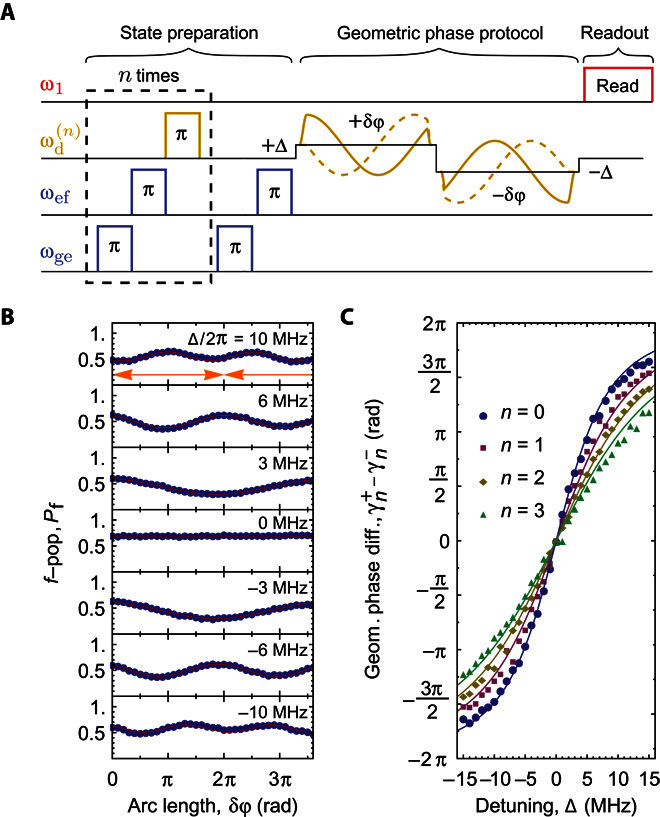
(A) Pulse sequence to detect the geometric phase difference accumulated between states $|{\mathrm{\Psi }}_{\mathit{n}}^{-}\rangle$ and $|{\mathrm{\Psi }}_{\mathit{n}}^{+}\rangle$ at finite detuning Δ. We first prepare the state |f, n〉, which is a superposition of $|{\mathrm{\Psi }}_{\mathit{n}}^{-}\rangle$ and $|{\mathrm{\Psi }}_{\mathit{n}}^{+}\rangle$. Then, we turn on the coupling and vary its phase by an amount δϕ. We repeat this operation twice, the second time with an opposite detuning −Δ, an opposite phase variation −δϕ, and a π phase shift. This sequence results in dynamic phase cancellation, whereas the different geometric phases accumulated by $|{\mathrm{\Psi }}_{\mathit{n}}^{\pm }\rangle$ can be detected as a population transfer away from the state |f, n〉. (B) Oscillations in the f-state population P_f as a function of the phase displacement δϕ, for selected values of the detuning Δ (circles, data; solid lines, sine fit) and n = 0 photons in the cavity. The phase of the oscillations when δϕ = 2π corresponds to the accumulated geometric phase in a single closed loop (whose extent is indicated by an orange line). (C) Geometric phase difference, $({\mathrm{\gamma }}_{\mathit{n}}^{+}-{\mathrm{\gamma }}_{\mathit{n}}^{-})$, versus detuning Δ for different photon numbers n (symbols). The solid lines are a simultaneous fit of the model expression (Eq. 2) to all data sets, with the coupling constant g as the only fit parameter.

In Fig. 4B, we plot representative traces of P_f versus δϕ, for n = 0 and different values of the detuning Δ. The experimental data (dots) are fitted to sinusoidal oscillations (solid lines). The acquired geometric phase γ after a full cycle (δϕ = 2π) is related to the frequency f of the oscillations (with respect to δϕ) by γ = πf. No oscillations are observed for Δ = 0. This is in agreement with the results presented in Fig. 3: at resonance, both states $|{\mathrm{\Psi }}_{\mathit{n}}^{\pm }\rangle$ acquire the same phase. As we move away from resonance, we observe oscillations of increasing frequency, indicating the accumulation of a geometric phase. The visibility of the oscillations decreases at higher detunings, due to our choice of |f0〉 as the reference state. In Fig. 4C, we plot the geometric phase difference $({\mathrm{\gamma }}_{\mathit{n}}^{+}-{\mathrm{\gamma }}_{\mathit{n}}^{-})$ versus the detuning Δ. Different symbols correspond to different photon numbers n = 0, 1, 2, and 3. We simultaneously fit our model expression (Eq. 2) to all data sets (solid lines), with the coupling constant g as the only fit parameter. The data are in good quantitative agreement with the model, with deviations on the order of a few percentages at large detunings and higher photon numbers. From the global fit, we extract the value g/2π = (4.49 ± 0.03) MHz. For comparison, an independent estimation based on Rabi oscillations gives g/2π = (4.12 ± 0.06) MHz (see the Supplementary Materials). We attribute the 8% discrepancy between these two values to a frequency-dependent attenuation in our input line (which includes a mixer and a room-temperature amplifier) and to higher-order transitions in our atom-cavity system, which are not accounted for in our model.

DISCUSSION

The Berry phase induced by a quantized field can be thought of as a nontrivial combination of the geometric phase acquired by a quantum two-level system (13) and that acquired by a harmonic oscillator (15). Our experiments provide clear evidence of this phase, thus putting the theory predictions by Fuentes-Guridi et al. (8) on a solid empirical basis and shedding light on a fundamental property of cavity quantum electrodynamics.

The techniques demonstrated here may open new avenues for the geometric manipulation of atom-cavity systems, including geometric control of cavity states (28–30) and cavity-assisted holonomic gates (16). For instance, our pulse scheme can be directly exploited to impart a geometric phase onto specific Fock states in the cavity, similarly to the results presented in a previous study (30). In our case, two consecutive, phase-shifted π pulses on the |f, n〉 ↔ |g, n + 1〉 transition realize a Fock state–selective phase gate in a time $\mathrm{\pi }/(\sqrt{\mathit{n}}\mathit{g})$, where g is the tunable coupling. Different Fock states can be simultaneously addressed by exploiting the cavity-induced Stark shift on the |f, n〉 ↔ |g, n + 1〉 transition, which is about 15 MHz in our system (see the Supplementary Materials). As a further application, the tunable coupling could be used to induce a cavity-mediated interaction between two transmons, paving the way for the realization of a two-qubit geometric gate based on non-Abelian holonomies (16).

MATERIALS AND METHODS

The microwave cavity used in this experiment was made of 6061 aluminum and had inner dimensions of 5 × 20 × 50 mm. The two lowest modes of the cavity had resonant frequencies ω₁/2π = 7.828 GHz and ω₂/2π = 9.041 GHz and quality factors Q₁ = 18,000 and Q₂ ≈ 3 × 10⁵. The next mode had a frequency ω₃/2π = 11.432 GHz.

The transmon was patterned onto a 4 × 7–mm sapphire chip with standard e-beam lithography, e-beam evaporation at different angles, and liftoff. It consists of two 200 × 300–μm Al pads separated by 160 μm and connected by a Josephson junction of Josephson energy E_J/h ≈ 35 GHz (16). The first two transition frequencies of the transmon are ω_ge/2π = 10.651 GHz and ω_ef/2π = 10.217 GHz. The decay time of both excited states is T₁ = (4.9 ± 0.1) μs, and their dephasing time is T₂** = (2.0 ± 0.1) μs.

All measurements were performed in a dilution refrigerator with a base temperature below 40 mK. The cavity was directly connected to a copper cold finger at the base plate. Additional copper braid was used to improve thermalization. The input line was attenuated by 60 dB between the 4-K stage and the input port of the cavity. In the output line, a high electron mobility transistor amplifier with 4-K nominal noise temperature was used as the first amplifier. The cavity output was isolated from the amplifier input with three isolators with at least 20-dB isolation each, thermalized below 150 mK. An 8- to 12-GHz bandpass filter was placed between the cavity output and the first isolator.

The pulses used to drive the transmon were generated by modulating coherent microwave tones with arbitrary waveforms using calibrated inphase-quadrature mixers. The signal from the output line was further amplified, down-converted into a 25-MHz signal, recorded with a fast digitizer, and averaged. The typical number of averages for the data presented in this paper is 60,000.

The qubit transition frequencies and the pulse amplitudes were determined by standard Rabi and Ramsey spectroscopy. When driving the transitions, we compensated for Stark shifts caused by the photonic occupation of the cavity mode (31) and the coupling field (24) (see the Supplementary Materials for a detailed discussion).

SUPPLEMENTARY MATERIALS

Supplementary material for this article is available at http://advances.sciencemag.org/cgi/content/full/2/5/e1501732/DC1

Characterization of the tunable coupling

Characterization at higher photon numbers

Geometric phases acquired by the eigenstates $|{\mathrm{\Psi }}_{\mathit{n}}^{\pm }\rangle$

Geometric phase estimation based on open loops

Dynamic phase cancellation

Insensitivity to small deviations from the resonant frequency

Phase calibration of spin-echo coupling pulses

fig. S1. Rabi spectroscopy of the tunable coupling.

fig. S2. Calibration of the strength and resonant frequency of the tunable coupling.

fig. S3. Calibration at higher photon numbers.

fig. S4. Geometric interpretation of the open-loop protocol.

REFERENCES AND NOTES

- 1.Xiao D., Chang M.-C., Niu Q., Berry phase effects on electronic properties. Rev. Mod. Phys. 82, 1959–2007 (2010). [Google Scholar]
- 2.Thouless D. J., Kohmoto M., Nightingale M. P., den Nijs M., Quantized Hall conductance in a two-dimensional periodic potential. Phys. Rev. Lett. 49, 405–408 (1982). [Google Scholar]
- 3.Hasan M. Z., Kane C. L., Colloquium: Topological insulators. Rev. Mod. Phys. 82, 3045–3067 (2010). [Google Scholar]
- 4.Qi X.-L., Zhang S.-C., Topological insulators and superconductors. Rev. Mod. Phys. 83, 1057–1110 (2011). [Google Scholar]
- 5.Zanardi P., Rasetti M., Holonomic quantum computation. Phys. Lett. A 264, 94–99 (1999). [Google Scholar]
- 6.Sjöqvist E., Trend: A new phase in quantum computation. Physics 1, 35 (2008). [Google Scholar]
- 7.Berry M. V., Quantal phase factors accompanying adiabatic changes. Proc. Roy. Soc. A 392, 45 (1984). [Google Scholar]
- 8.Fuentes-Guridi I., Carollo A., Bose S., Vedral V., Vacuum induced spin-1/2 Berry’s phase. Phys. Rev. Lett. 89, 220404 (2002). [DOI] [PubMed] [Google Scholar]
- 9.Liu T., Feng M., Wang K., Vacuum-induced Berry phase beyond the rotating-wave approximation. Phys. Rev. A 84, 062109 (2011). [Google Scholar]
- 10.Larson J., Absence of vacuum induced Berry phases without the rotating wave approximation in cavity QED. Phys. Rev. Lett. 108, 033601 (2012). [DOI] [PubMed] [Google Scholar]
- 11.Wang M., Wei L., Liang J., Does the Berry phase in a quantum optical system originate from the rotating wave approximation? Phys. Lett. A 379, 1087–1090 (2015). [Google Scholar]
- 12.Falci G., Fazio R., Palma G. M., Siewert J., Vedral V., Detection of geometric phases in superconducting nanocircuits. Nature 407, 355–358 (2000). [DOI] [PubMed] [Google Scholar]
- 13.Leek P. J., Fink J. M., Blais A., Bianchetti R., Göppl M., Gambetta J. M., Schuster D. I., Frunzio L., Schoelkopf R. J., Wallraff A., Observation of Berry’s phase in a solid-state qubit. Science 318, 1889–1892 (2007). [DOI] [PubMed] [Google Scholar]
- 14.Möttönen M., Vartiainen J. J., Pekola J. P., Experimental determination of the Berry phase in a superconducting charge pump. Phys. Rev. Lett. 100, 177201 (2008). [DOI] [PubMed] [Google Scholar]
- 15.Pechal M., Berger S., Abdumalikov A. A. Jr, Fink J. M., Mlynek J., Steffen L., Wallraff A., Filipp S., Geometric phase and nonadiabatic effects in an electronic harmonic oscillator. Phys. Rev. Lett. 108, 170401 (2012). [DOI] [PubMed] [Google Scholar]
- 16.Abdumalikov A. A. Jr, Fink J. M., Juliusson K., Pechal M., Berger S., Wallraff A., Filipp S., Experimental realization of non-Abelian non-adiabatic geometric gates. Nature 496, 482–485 (2013). [DOI] [PubMed] [Google Scholar]
- 17.Berger S., Pechal M., Abdumalikov A. A. Jr, Eichler C., Steffen L., Fedorov A., Wallraff A., Filipp S., Exploring the effect of noise on the Berry phase. Phys. Rev. A 87, 060303 (2013). [Google Scholar]
- 18.Roushan P., Neill C., Chen Y., Kolodrubetz M., Quintana C., Leung N., Fang M., Barends R., Campbell B., Chen Z., Chiaro B., Dunsworth A., Jeffrey E., Kelly J., Megrant A., Mutus J., O’Malley P. J. J., Sank D., Vainsencher A., Wenner J., White T., Polkovnikov A., Cleland A. N., Martinis J. M., Observation of topological transitions in interacting quantum circuits. Nature 515, 241–244 (2014). [DOI] [PubMed] [Google Scholar]
- 19.Schroer M. D., Kolodrubetz M. H., Kindel W. F., Sandberg M., Gao J., Vissers M. R., Pappas D. P., Polkovnikov A., Lehnert K. W., Measuring a topological transition in an artificial spin-1/2 system. Phys. Rev. Lett. 113, 050402 (2014). [DOI] [PubMed] [Google Scholar]
- 20.Jones J. A., Vedral V., Ekert A., Castagnoli G., Geometric quantum computation using nuclear magnetic resonance. Nature 403, 869–871 (2000). [DOI] [PubMed] [Google Scholar]
- 21.Bose S., Carollo A., Fuentes-guridi I., Santos M. F., Vedral V., Vacuum induced berry phase: Theory and experimental proposal. J. Mod. Opt. 50, 1175–1181 (2003). [Google Scholar]
- 22.Liu Y., Wei L. F., Jia W. Z., Liang J. Q., Vacuum-induced Berry phases in single-mode Jaynes-Cummings models. Phys. Rev. A 82, 045801 (2010). [Google Scholar]
- 23.Pechal M., Huthmacher L., Eichler C., Zeytinoğlu S., Abdumalikov A. A. Jr, Berger S., Wallraff A., Filipp S., Microwave-controlled generation of shaped single photons in circuit quantum electrodynamics. Phys. Rev. X 4, 041010 (2014). [Google Scholar]
- 24.Zeytinoğlu S., Pechal M., Berger S., Abdumalikov A. A. Jr, Wallraff A., Filipp S., Microwave-induced amplitude- and phase-tunable qubit-resonator coupling in circuit quantum electrodynamics. Phys. Rev. A 91, 043846 (2015). [Google Scholar]
- 25.Paik H., Schuster D. I., Bishop L. S., Kirchmair G., Catelani G., Sears A. P., Johnson B. R., Reagor M. J., Frunzio L., Glazman L. I., Girvin S. M., Devoret M., Schoelkopf R. J., Observation of high coherence in Josephson junction qubits measured in a three-dimensional circuit QED architecture. Phys. Rev. Lett. 107, 240501 (2011). [DOI] [PubMed] [Google Scholar]
- 26.Bianchetti R., Filipp S., Baur M., Fink J. M., Lang C., Steffen L., Boissonneault M., Blais A., Wallraff A., Control and tomography of a three level superconducting artificial atom. Phys. Rev. Lett. 105, 223601 (2010). [DOI] [PubMed] [Google Scholar]
- 27.Samuel J., Bhandari R., General setting for Berry’s phase. Phys. Rev. Lett. 60, 2339–2342 (1988). [DOI] [PubMed] [Google Scholar]
- 28.Vlastakis B., Kirchmair G., Leghtas Z., Nigg S. E., Frunzio L., Girvin S. M., Mirrahimi M., Devoret M., Schoelkopf R. J., Deterministically encoding quantum information using 100-photon Schrödinger cat states. Science 342, 607–610 (2013). [DOI] [PubMed] [Google Scholar]
- 29.Albert V. V., Shu C., Krastanov S., Shen C., Liu R.-B., Yang Z.-B., Schoelkopf R. J., Mirrahimi M., Devoret M. H., Jiang L., Holonomic quantum control with continuous variable systems. Phys. Rev. Lett. 116, 140502 (2016). [DOI] [PubMed] [Google Scholar]
- 30.Heeres R. W., Vlastakis B., Holland E., Krastanov S., Albert V. V., Frunzio L., Jiang L., Schoelkopf R. J., Cavity state manipulation using photon-number selective phase gates. Phys. Rev. Lett. 115, 137002 (2015). [DOI] [PubMed] [Google Scholar]
- 31.Schuster D. I., Houck A. A., Schreier J. A., Wallraff A., Gambetta J. M., Blais A., Frunzio L., Majer J., Johnson B., Devoret M. H., Girvin S. M., Schoelkopf R. J., Resolving photon number states in a superconducting circuit. Nature 445, 515–518 (2007). [DOI] [PubMed] [Google Scholar]
Associated Data
This section collects any data citations, data availability statements, or supplementary materials included in this article.