Noise-immune complex correlation for optical coherence angiography based on standard and Jones matrix optical coherence tomography

Abstract

This paper describes a complex correlation mapping algorithm for optical coherence angiography (cmOCA). The proposed algorithm avoids the signal-to-noise ratio dependence and exhibits low noise in vasculature imaging. The complex correlation coefficient of the signals, rather than that of the measured data are estimated, and two-step averaging is introduced. Algorithms of motion artifact removal based on non perfusing tissue detection using correlation are developed. The algorithms are implemented with Jones-matrix OCT. Simultaneous imaging of pigmented tissue and vasculature is also achieved using degree of polarization uniformity imaging with cmOCA. An application of cmOCA to in vivo posterior human eyes is presented to demonstrate that high-contrast images of patients’ eyes can be obtained.

1. Introduction

Optical coherence angiography (OCA) is a non-invasive vasculature contrast technique based on optical coherence tomography (OCT). OCA has been used in several applications, e.g., ophthalmology [1–5], oncology [6], neurology [7], and gastroenterology [8]. Several angiography methods and algorithms have been developed, including OCA based on Doppler phase-shift detection [9–11], high-pass filtering techniques [12–18], intensity variance [19], and phase-shift variance [20, 21]. Methods based on intensity correlation [22–24] and complex correlation [6, 25–27] have also been presented. Among these, the complex-correlation-based technique uses all of the complex information of OCT, and provides good vasculature contrast [27]. In addition, the correlation-based methods are sensitive to the mobility of scatterers and less sensitive to the Doppler angle [28].

Despite these advantages, complex-correlation-based OCA still suffers from certain problems. First, the correlation coefficient is not only affected by motion, but also by the signal-to-noise ratio (SNR) [29]; i.e., low SNRs create artificially high flow signals. A signal-intensity-based threshold has been widely used to remove the low-SNR regions [20, 24, 27, 30], but the correlation signals above the threshold are still affected by the SNR, and this approach is not fully quantitative. The second point is the variance of the estimated complex correlation coefficient. This is limiting the contrast of vasculature imaging. For in vivo imaging, the involuntary motion of samples causes decorrelation and artifacts.

In this paper, a new OCA method, which we call correlation mapping OCA (cmOCA), is derived using the SNR-corrected low-noise complex correlation. We present SNR-correction and variance-reduction theories for the complex correlation coefficient estimation (Section 2). The treatment of bulk tissue motion is described in Section 3.1 and Section 3.2. The cmOCA method is applied with Jones matrix OCT (JM-OCT) [31–37], which is a type of polarization-sensitive OCT that has multiple polarization detection channels and enables polarization-sensitive contrast. Details of the implementation of cmOCA with JM-OCT are presented in Section 4. The combination of degree-of-polarization uniformity (DOPU) and cmOCA for simultaneous visualization of vasculature and the retinal pigment epithelium (RPE) in the eye (Section 5.3) is also described. The cmOCA method is applied to normal and pathologic eyes.

2. Theory of SNR-corrected low-noise complex correlation coefficient estimates

In this section, the general complex correlation coefficient of OCT signal and its estimate are derived (Section 2.1). The SNR-corrected low-noise estimator of the complex correlation coefficient is then described (Section 2.2). The notations used here and the following sections are listed in Appendix B.

2.1. Complex correlation of OCT signals

By assuming that the OCT signal at the spatiotemporal point r = (x, z, t) (where x is the transversal position, z is the axial position, and t is time) is a random variable G(r), the covariance matrix between two OCT signals at r and r + Δr can be expressed as

$${\mathrm{\Sigma }}_G(\mathrm{\Delta }\mathbf{r};\mathbf{r})=\left[\begin{array}{cc}\mathrm{E}\left[{\left|G(\mathbf{r})\right|}^2\right]& \mathrm{E}\left[G(\mathbf{r})G*(\mathbf{r}+\mathrm{\Delta }\mathbf{r})\right]\\ \mathrm{E}\left[G(\mathbf{r}+\mathrm{\Delta }\mathbf{r})G*(\mathbf{r})\right]& \mathrm{E}\left[{\left|G(\mathbf{r}+\mathrm{\Delta }\mathbf{r})\right|}^2\right]\end{array}\right],$$ (1)

where E[ ] represents the expectation, and E[G(r)] is assumed to be zero. The population correlation coefficient ρ_G and phase offset θ_G between G(r) and G(r + Δr) are

$${\rho }_G(\mathrm{\Delta }\mathbf{r};\mathbf{r})e^{i{\theta }_G(\mathrm{\Delta }\mathbf{r};\mathbf{r})}=\frac{\mathrm{E}[G(\mathbf{r})G*(\mathbf{r}+\mathrm{\Delta }\mathbf{r})]}{\sqrt{\mathrm{E}\left[{\left|G(\mathbf{r})\right|}^2\right]\mathrm{E}\left[{\left|G(\mathbf{r}+\mathrm{\Delta }\mathbf{r})\right|}^2\right]}}$$ (2)

The correlation coefficient ρ_G is estimated using the sample covariance matrix S_G between the measured OCT signal pair g(r) and g(r + Δr) which is obtained as

$$\begin{array}{ll}{\mathbf{S}}_G(\mathrm{\Delta }\mathbf{r};\mathbf{r})& \equiv {\langle \mathbf{g}(\mathrm{\Delta }\mathbf{r};\mathbf{r}){\mathbf{g}}^{†}(\mathrm{\Delta }\mathbf{r};\mathbf{r})\rangle }_{w_1}\\ & ={\langle \left[\begin{array}{cc}{\left|g(\mathbf{r})\right|}^2& g(\mathbf{r})g*(\mathbf{r}+\mathrm{\Delta }\mathbf{r})\\ g*(\mathbf{r})g(\mathbf{r}+\mathrm{\Delta }\mathbf{r})& {\left|g(\mathbf{r}+\mathrm{\Delta }\mathbf{r})\right|}^2\end{array}\right]\rangle }_{w_1},\end{array}$$ (3)

where

$$\mathbf{g}(\mathrm{\Delta }\mathbf{r};\mathbf{r})=\left[\begin{array}{c}g(\mathbf{r})\\ g(\mathbf{r}+\mathrm{\Delta }\mathbf{r})\end{array}\right],$$ (4)

and 〈·〉_w is an averaging operation across a window w. The superscript ^† denotes the conjugate transpose operation. The correlation coefficient estimate of ρ_G is then obtained as

$$r_G(\mathrm{\Delta }\mathbf{r};\mathbf{r})\equiv {\hat{\rho }}_G(\mathrm{\Delta }\mathbf{r};\mathbf{r})\equiv \frac{\left|s_{G12}\right|}{\sqrt{s_{G11}\cdot s_{G22}}},$$ (5)

where s_Gpq are the entry of the estimated covariance matrix S_G at p-th row and q-th column.

In practical OCT measurements, the correlation coefficients obtained from measured OCT signals are not only affected by the true OCT signal, but also by noise. The OCT signal to be measured at the spatiotemporal point r can be considered as the summation of the true OCT signal S(r) and some random additive noise N:

$$G(\mathbf{r})=S(\mathbf{r})+N.$$ (6)

By assuming S(r) to be a zero-mean process and N to be a zero-mean stationary random process, the covariance matrix [Eq. (1)] can be written as

$${\mathrm{\Sigma }}_G(\mathrm{\Delta }\mathbf{r};\mathbf{r})=\left[\begin{array}{cc}\mathrm{E}\left[{\left|S(\mathbf{r})\right|}^2\right]+\mathrm{E}\left[{\left|N\right|}^2\right]& \mathrm{E}\left[S*(\mathbf{r})S(\mathbf{r}+\mathrm{\Delta }\mathbf{r})\right]\\ \mathrm{E}\left[S*(\mathbf{r}+\mathrm{\Delta }\mathbf{r})S(\mathbf{r})\right]& \mathrm{E}\left[{\left|S(\mathbf{r}+\mathrm{\Delta }\mathbf{r})\right|}^2\right]+\mathrm{E}\left[{\left|N\right|}^2\right].\end{array}\right]$$ (7)

The correlation between measured OCT signals at different spatiotemporal points, ρ_G(Δr;r), can then be written as the product of the correlation coefficient of the true OCT signals, ρ_S(Δr;r), and a factor expressing the noise effect, ρ_SNR(Δr;r), as [29]

$${\rho }_G(\mathrm{\Delta }\mathbf{r};\mathbf{r})={\rho }_{\text{SNR}}(\mathrm{\Delta }\mathbf{r};\mathbf{r}){\rho }_S(\mathrm{\Delta }\mathbf{r};\mathbf{r}),$$ (8)

where

$${\rho }_S(\mathrm{\Delta }\mathbf{r};\mathbf{r})=\frac{\mathrm{E}[S*(\mathbf{r})S(\mathbf{r}+\mathrm{\Delta }\mathbf{r})]}{\sqrt{\mathrm{E}\left[{\left|S(\mathbf{r})\right|}^2\right]}\sqrt{\mathrm{E}\left[{\left|S(\mathbf{r}+\mathrm{\Delta }\mathbf{r})\right|}^2\right]}}$$ (9)

$${\rho }_{\text{SNR}}(\mathrm{\Delta }\mathbf{r};\mathbf{r})={\left[\sqrt{1+\text{SNR}{(\mathbf{r})}^{-1}}\sqrt{1+\text{SNR}{(\mathbf{r}+\mathrm{\Delta }\mathbf{r})}^{-1}}\right]}^{-1}.$$ (10)

ρ_SNR(Δr; r) [Eq. (10)] is a decorrelation factor caused by the random noise, where SNR(r) = E[|S(r)|²]/E[|N|²]. Hence, r_G [Eq. (5)] does not provide an accurate estimate of the signal correlation ρ_S.

The bias $b_{r_G}$ and variance ${\sigma }_{r_G}$ in the correlation estimate r_G are expressed as

$$b_{r_G}=\mathrm{E}[r_G]-{\rho }_S,$$ (11)

$${\sigma }_{r_G}=\mathrm{E}[r_G^2]-\mathrm{E}{[r_G]}^2.$$ (12)

The bias decreases with higher SNRs. As SNR → ∞, ρ_SNR → 1 and ρ_G → ρ_S. Thus, the bias $b_{r_G}$ decreases. However, the variance of estimation is not always small at high SNRs. The variance ${\sigma }_{r_G}$ depends on ρ_G, and rapidly increases as ρ_G decreases [38, 39]. Hence, the variance is large with small ρ_S even when the SNR is high (Table 1). The large variance ${\sigma }_{r_G}$ will results in the noise of the correlation imaging.

Table 1.

Variance of correlation coefficient estimation ${\sigma }_{r_G}$.

ρS	low	≈ 1
SNR
high	high	low
low	high	high

2.2. SNR-corrected low-bias, low-noise complex correlation estimation

The correlation of signal ρ_S(Δr;r) can be estimated using the noise power estimation technique presented in our previous studies [29, 40]. In the present paper, we further modify this method to achieve a lower estimation noise than the previous approach.

The signal correlation was estimated as

$$r_S(\mathrm{\Delta }\mathbf{r};\mathbf{r})\equiv \frac{\left|s_{G12}\right|}{\sqrt{|[s_{G11}-{\hat{q}}_N][s_{G22}-{\hat{q}}_N]|}},$$ (13)

where s_Spq are the entry of the estimated covariance matrix S_S at p-th row and q-th column, and ${\hat{q}}_N$ is an estimation of the noise power, obtained as

$${\hat{q}}_N\equiv {\langle {\left|g_n(t)-{\langle g_n(t)\rangle }_t\right|}^2\rangle }_t,$$ (14)

where 〈 〉_t denotes time-averaging. g_n(t) is the measured OCT signal obtained without a sample. This can be pre-determined by blocking the probe beam, or can be estimated from tissue measurement data using OCT signals from non-tissue regions. Here, we assume the noise N is identical in space. However, some OCT systems have a depth-dependent noise power. In this case, the noise power ${\hat{q}}_N$ should be treated as a function of depth z. The SNR-correction, however, does not reduce the variance of the estimation.

To reduce the estimation noise, a second averaging is applied to estimate the magnitude of the covariance and the geometric mean of variances. A correlation estimate with lower noise than Eq. (5) can be obtained using an averaging window w₂ as

$${\overline{r}}_G(\mathrm{\Delta }\mathbf{r};\mathbf{r})\equiv \frac{{\langle \left|s_{G12}\right|\rangle }_{w_2}}{{\langle \sqrt{s_{G11}\cdot s_{G22}}\rangle }_{w_2}}.$$ (15)

Similarly, a low-noise signal correlation estimate is obtained from Eq. (13) as

$${\overline{r}}_S(\mathrm{\Delta }\mathbf{r};\mathbf{r})\equiv \frac{{\langle \left|s_{G12}\right|\rangle }_{w_2}}{{\langle \epsilon \sqrt{|[s_{G11}-{\hat{q}}_N][s_{G22}-{\hat{q}}_N]|}\rangle }_{w_2}},$$ (16)

where

$$\epsilon =\frac{\mathrm{sgn}(s_{G11}-{\hat{q}}_N)+\mathrm{sgn}(s_{G22}-{\hat{q}}_N)}{2}.$$ (17)

The sign ε is applied to suppress the bias of the denominator of Eq. (16) after the averaging ${\langle \rangle }_{w_2}$ when the signal is zero (See Section 7). Note that the estimate of Eq. (16) can be negative or exceed 1. For imaging, the range of estimate ${\overline{r}}_S$ will be wrapped as described in Section 5.1.

3. Correlation mapping optical coherence angiography

The present paper aims to demonstrate high-contrast OCA using the correlation coefficient of the true OCT signal, as shown in Section 2.2. We refer to this as correlation mapping OCA (cmOCA).

Typically, a single location on the sample is scanned multiple times, and the temporal correlation is calculated to contrast the blood flow. The temporal correlation between time points t and t +τ at space point (x, z) is denoted as ρ_S(Δr;r)|_Δr=(0,0,τ) in the notation of Section 2. Hereafter, this is denoted as ρ_S(τ;r) for simplicity.

During the estimation of the temporal correlation coefficient, temporal averaging will be applied, and then the spatial distribution of the signal correlation coefficient is obtained, ${\overline{r}}_S({\mathbf{r}}_i,{\mathbf{r}}_j)\to {\overline{r}}_S(\tau ;\mathbf{x},z)$. This can be described as

$${\overline{r}}_S(\tau ;\mathbf{x},z)\equiv \frac{{\langle \left|{\langle g(\mathbf{r})g*(\mathbf{r}+(\mathbf{0},0,\tau ))\rangle }_{w_1}\right|\rangle }_{w_2}}{{\langle \epsilon \sqrt{\left|\left[{\langle {\left|g(\mathbf{r})\right|}^2\rangle }_{w_1}-{\hat{q}}_N\right]\left[{\langle {\left|g(\mathbf{r}+(\mathbf{0},0,\tau ))\right|}^2\rangle }_{w_1}-{\hat{q}}_N\right]\right|}\rangle }_{w_2}}.$$ (18)

Two specific issues for in vivo cmOCA measurements are also discussed. These are associated with the bulk sample motion. The first issue is the bulk phase offset caused by the axial shift of the sample between the two time points for which the correlation is computed. Two approaches to avoid this bulk phase offset are described in Section 3.1. The second issue is the reduction in the correlation coefficient due to the general bulk motion of the sample. This creates artifacts, which affect our primary interest of visualizing only the region with real blood flow. Section 3.2 presents a method to remove such artifacts. The processing flow is described as a block diagram in Fig. 1.

Fig. 1.

Schematic block diagrams of cmOCA processing. (a) Overall processing. (b) Covariance matrix estimate with bulk-phase-offset correction.

3.1. Bulk-motion-induced phase-offset problem

The bulk motion of tissues induces a substantial phase shift, and this significantly decreases the correlation coefficient when the averaging window ${\langle \rangle }_{w_1}$ in Eq. (18) is extended along the temporal direction. There are two approaches to overcome this problem. One is to apply a bulk-phase-offset correction to the estimation and the other is to form an estimation that is insensitive to the bulk-phase-offset.

3.1.1. Bulk-phase-offset correction

To eliminate the bulk-motion effect, we must detect the magnitude of the bulk-phase offset. For this purpose, previous studies have introduced sophisticated methods [9, 11, 41–43]. Although these methods exhibit high detection accuracy, they also suffer from high computational costs. Some simpler methods have been used for vasculature imaging [20, 44–46], but their use is limited to specific cases, such as when the non perfused region is dominant in each axial profile.

Here, we describe a simple and robust bulk-phase-offset correction method. The key of this method is the estimation of locations of non-perfused tissue. The non perfused region is selected for each axial profile using the characteristics of data correlation coefficient ρ_G. According to the relationship between correlation and SNR [Eq. (8)], locations with high correlation coefficient ρ_G, are very likely to be tissue without perfusion and simultaneously to have high SNRs. Such high SNRs are preferable for the reliable estimation of the bulk-phase offset. The relationship is summarized in Table 2.

Table 2.

Correlation coefficient ρ_G for each tissue type and SNR.

Type	non perfused tissue	flowing particles
SNR
high	high	low
low	low–moderate	low

To implement this method, the covariance matrix estimation process [Eq. (3)] is resolved in two steps, i.e., bulk-phase-offset estimation and averaging after the phase correction. A block diagram of this processing framework is shown in Fig. 1(b). In the first step, a sample covariance matrix similar to Eq. (3) is estimated as:

$${\mathbf{S}}_G^{\prime }(\tau ;\mathbf{r})\equiv {\langle \mathbf{g}(\tau ;\mathbf{r}){\mathbf{g}}^{†}(\tau ;\mathbf{r})\rangle }_{w_1^{\prime }}.$$ (19)

and the data correlation ${\overline{r}}_G^{\prime }$ is then estimated using Eqs. (15) as

$${\overline{r}}_G^{\prime }(\tau ;\mathbf{r})\equiv \frac{{\langle \left|s_{G12}^{\prime }\right|\rangle }_{w_2^{\prime }}}{{\langle \sqrt{s_{G11}^{\prime }\cdot s_{G22}^{\prime }}\rangle }_{w_2^{\prime }}}.$$ (20)

To prevent the disruption caused by bulk-phase offset, the estimation ${\langle \rangle }_{w_1^{\prime }}$ of Eq. (19) should be computed by time-independent averaging, e.g., axial averaging. The bulk-phase offset between time points t and t + τ is then determined at depth z^max(τ; x, t), which exhibits a high value of ${\overline{r}}_G^{\prime }$ at x, as

$$\mathrm{\Delta }{\varphi }_m(\tau ;\mathbf{x},t)\equiv \arg \left\{{\langle s_{G12}^{\prime }(\tau ;\mathbf{r}{|}_{z=z^{\max }(\tau ;\mathbf{x},t)})\rangle }_{w_3}\right\}.$$ (21)

Using Eq. (21), the bulk-phase-offset is corrected and the covariance matrix is finally estimated as

$${\mathbf{S}}_G(\tau ;\mathbf{x},z)\equiv {\langle \left[\begin{array}{cc}{s}_{G11}^{\prime }& s_{G12}^{\prime }{e}^{-i\mathrm{\Delta }{\varphi }_m(\tau ;\mathbf{x},t)}\\ {\left\{s_{G12}^{\prime }{e}^{-i\mathrm{\Delta }{\varphi }_m(\tau ;\mathbf{x},t)}\right\}}^{*}& s_{G22}^{\prime }\end{array}\right]\rangle }_{w_1^{″}}.$$ (22)

The signal correlation map ${\overline{r}}_S(\tau ;\mathbf{x},z)$ is estimated by substituting Eqs. (19) and (21) to (22) into Eq. (16) as

$${\overline{r}}_S(\tau ;\mathbf{x},z)\equiv \frac{{\langle \left|{\langle {\langle g(\mathbf{r})g*(\mathbf{r}+(\mathbf{0},0,\tau ))\rangle }_{w_1^{\prime }}{e}^{-i\mathrm{\Delta }{\varphi }_m(\tau ;\mathbf{x},\tau )}\rangle }_{w_1^{″}}\right|\rangle }_{w_2}}{{\langle \epsilon \sqrt{\left|\left[{\langle {\langle {\left|g(\mathbf{r})\right|}^2\rangle }_{w_1^{\prime }}\rangle }_{w_1^{″}}-{\hat{q}}_N\right]\left[{\langle {\langle {\left|g(\mathbf{r}+(\mathbf{0},0,\tau ))\right|}^2\rangle }_{w_1^{\prime }}\rangle }_{w_1^{″}}-{\hat{q}}_N\right]\right|}\rangle }_{w_2}}.$$ (23)

3.1.2. Phase-noise-immune estimate

In the case of swept-source OCT (SS-OCT) systems, the phase fluctuations caused by asynchronous acquisition [47] and/or random phase noise of coherence revival signals [48] make it difficult to acquire phase-stable signals. In addition, when no k-clock is used [49], the low repeatability of the wavelength sweep of a light source could further degrade the phase stability.

In such cases, another algorithm with phase-noise immunity is applied. The sample covariance matrix S_G is estimated as similar to Eq. (3) as:

$${\mathbf{S}}_G(\tau ;\mathbf{r})\equiv {\langle \mathbf{g}(\tau ;\mathbf{r}){\mathbf{g}}^{†}(\tau ;\mathbf{r})\rangle }_{w_1}.$$ (24)

To minimize the effect of the phase fluctuation, the averaging window w₁ is selected within time independent region as in Eq. (19). One example is axial averaging [27].

3.2. Removal of bulk-motion artifacts

Motion artifacts can occur in cmOCA images as a result of the de-correlation due to involuntary eye motion. This section describes a method to remove these artifacts from correlation coefficient estimates which is obtained without bulk-phase-offset problem (Section 3.1).

If the bulk tissue motion is rigid translation, and its velocity is quite smaller than the net blood velocity, the correlation ρ_S(τ;r) can be decomposed as

$${\rho }_S(\tau ;\mathbf{r})\approx {\rho }_f(\tau ;\mathbf{r}){\rho }_m(\tau ;\mathbf{x},t),$$ (25)

where ρ_f (τ; r) is the correlation coefficient corresponding to blood flow. This is mainly caused by the motion of blood cells. ρ_m(τ; x, t) is the correlation coefficient corresponding to bulk motion, which is uniform along the axial direction because single axial profiles are acquired simultaneously by Fourier-domain OCT. By assuming the bulk tissue motion velocity is constant during the temporal estimate window of correlation, the correlation estimate ${\overline{r}}_S(\tau ;\mathbf{x},z)$ can be expressed as

$${\overline{r}}_S(\tau ;\mathbf{x},z)\approx {\tilde{r}}_f(\tau ;\mathbf{x},z)r_m(\tau ;\mathbf{x}),$$ (26)

where ${\tilde{r}}_f(\tau ;\mathbf{x},z)$ is the net correlation coefficient corresponding to blood flow. The reduction of ${\overline{r}}_S(\tau ;\mathbf{x},z)$ due to r_m(τ; x) is the source of the bulk motion artifacts. Because the correlation coefficient is estimated with bulk-phase-offset correction (Section 3.1.1) or phase-noise-immune estimate (Section 3.1.2), decorrelation due to bulk-phase-offset is avoided. Our motion-artifact-correction method first estimates r_m(τ; x), and then removes this quantity from ${\overline{r}}_S(\tau ;\mathbf{x},z)$.

As discussed in Section 3.1.1, tissue with a higher data correlation is more likely to be non perfused tissue with a high SNR. For such non perfused tissue, the correlation coefficient estimate ${\overline{r}}_S(\tau ;\mathbf{x},z)$ will be identical to r_m(τ; x), so ${\overline{r}}_S(\tau ;\mathbf{x},z)$ in the non perfused tissue can be used to cancel out the bulk motion artifacts. The correlation coefficient ${\overline{r}}_G(\tau ;\mathbf{x},z)$ is obtained from the covariance matrix estimate S_G [Eq. (22) or (24)] in the manner of Eq. (15) as

$${\overline{r}}_G(\tau ;\mathbf{x},z)\equiv \frac{{\langle \left|s_{G12}\right|\rangle }_{w_2}}{{\langle \sqrt{s_{G11}{s}_{G22}}\rangle }_{w_2}}.$$ (27)

Hence, the signal correlation estimate ${\overline{r}}_S$ at the depth of the maximum of ${\overline{r}}_G(\tau ;\mathbf{x},z)$ is used as an estimate of r_m:

$${\hat{r}}_m(\tau ;\mathbf{x})\equiv {\overline{r}}_S(\tau ;\mathbf{x},\underset{Z}{\arg \max }{\overline{r}}_G(\tau ;\mathbf{x},z)).$$ (28)

The bulk-motion-corrected signal correlation coefficient is finally obtained as

$${\overline{r}}_{Sf}(\tau ;\mathbf{x},z)\equiv \frac{{\overline{r}}_S(\tau ;\mathbf{x},z)}{{\hat{r}}_m(\tau ;\mathbf{x})}.$$ (29)

This estimate represents the correlation due to flow, and is used to form bulk-motion-corrected cmOCA images.

4. Method

In this paper, we use Jones matrix OCT (JM-OCT), which is a multi-channel extension of OCT. JM-OCT was originally developed for polarization-sensitive imaging [31–33,50] and has recently been applied to multifunctional imaging [1, 49, 51].

First, we describe the scanning protocol for cmOCA measurements, and re-define variables to indicate sampling points (Section 4.1). The details of cmOCA implementations with JM-OCT is then described (Section 4.2).

4.1. Measurement protocol and correlation for cmOCA

For cmOCA measurements, multiple frames (B-scans) are obtained from the same position on the sample. The schematic diagram of these sampling points is shown in Fig. 2. A single location on the sample is scanned multiple times by this scanning protocol. The correlation is computed at each spatial position among the frames.

Fig. 2.

Schematic diagram of applied scanning protocol.

JM-OCT simultaneously provides four independent OCT signals [49]. These are denoted as g(x, z, f, p), where f is the index of frame and p = 1,2,3,4 is the index of the JM-OCT channels. Note that variables x and z are re-defined as sampling point indices along the lateral and axial directions, respectively. The time correlation between frames f and f + 1 at space point (x, z) of p channel is denoted as ρ_S(τ; x, z, f, p), where τ is the time separation between successive frames. The correlations, covariance matrices, and their estimates are denoted in the same manner.

4.2. cmOCA implementation with JM-OCT

To obtain lower bias in correlation estimate, a large number of samples is required to estimate the covariance matrix [Eq. (3)]. To increase the size of the average ${\langle \rangle }_{w_1}$, the bulk-phase-offset correction (Section 3.1.1) is preferable to extend the window w₁ along temporal axis. Each averaging operation in the pre-processing of the bulk-phase-offset estimate [Eqs. (19) and (20)] is replaced according to Table 3 as

$${{\mathbf{S}}^{\prime }}_G^{\mathrm{M}}(\tau ;x,z,f,p)\equiv \frac{1}{D}{\displaystyle \sum _d^D\mathbf{g}(\tau ;x,z+d,f,p){\mathbf{g}}^{†}(\tau ;x,z+d,f,p)}$$ (30)

$${{\overline{r}}^{\prime }}_G^{\mathrm{M}}(\tau ;x,z,f)\equiv \frac{{\displaystyle {\sum }_p^P\frac{1}{{\hat{q}}_N(p)}\left|{s^{\prime }}_{G12}^{\mathrm{M}}\right|}}{{\displaystyle {\sum }_p^P\frac{1}{{\hat{q}}_N(p)}\sqrt{{s^{\prime }}_{G11}^{\mathrm{M}}{s^{\prime }}_{G22}^{\mathrm{M}}}}},$$ (31)

where D is the size of the averaging kernel along the axial direction. Here, we have used the K pixels with the highest correlation coefficients ${{\overline{r}}^{\prime }}_G^{\mathrm{M}}$ in each axial profile to estimate the bulk-phase offset. The axial indices of these pixels are denoted as $z_k^{\max }(\tau ;x,f)$, with the index k identifying these pixels as k = 1,⋯,K. As in Eq. (21), the bulk-phase-offset estimate is obtained from ${s^{\prime }}_{G12}^{\mathrm{M}}(\tau ;x,z,f,p)$ at depths $z_k^{\max }(\tau ;x,f)$ as

$$\mathrm{\Delta }{\varphi }_m^{\mathrm{M}}(\tau ;x,f)\equiv \arg \left\{\underset{x}{\text{Med}}\left[\frac{1}{PK}{\displaystyle \sum _p^P{\displaystyle \sum _{k=1}^K{s^{\prime }}_{G12}^{\mathrm{M}}(\tau ;x,z_k^{\max }(\tau ;x,f),f,p)}}\right]\right\},$$ (32)

where $\underset{x}{\text{Med}}[\cdot ]$ represents the median operation along the transverse (x-) direction, which is independently applied to the real and imaginary parts. In this paper, we consider K = 5, and select ±15 lines to compute the median $\underset{x}{\text{Med}}$. The bulk-phase-offset correction is applied to ${{\mathbf{S}}^{\prime }}_G^{\mathrm{M}}$ [Eq. (30)] with Eq. (32). The covariance matrix estimate is obtained with lateral and frame averaging for ${\langle \rangle }_{w_1^{″}}$. The correlation coefficient estimate is then described from Eq. (23) using the noise power of each channel ${\hat{q}}_N(p)$ as

$${\overline{r}}_S^{\mathrm{M}}(\tau ;x,z)\equiv \frac{{\displaystyle {\sum }_p\frac{1}{{\hat{q}}_N(p)}\left|{\displaystyle {\sum }_{l,d,f}^{L,D,F-1}g(x+l,z+d,f,p)g*(x+l,z+d,f+1,p)e^{-i\mathrm{\Delta }{\varphi }_m^{\mathrm{M}}(\tau ;x+l,f)}}\right|}}{\begin{array}{r}{\displaystyle {\sum }_p\frac{\epsilon (x,z,p)}{{\hat{q}}_N(p)}}\{|\left[{\displaystyle {\sum }_{l,d,f}^{L,D,F-1}{\left|g(x+l,z+d,f,p)\right|}^2}-LD(F-1){\hat{q}}_N(p)\right]\\ {\times \left[{\displaystyle {\sum }_{l,d,f}^{L,D,F-1}{\left|g(x+l,z+d,f+1,p)\right|}^2}-LD(F-1){\hat{q}}_N(p)\right]|\}}^{\frac{1}{2}}\end{array}},$$ (33)

where L is the size of the averaging kernel along the lateral direction.

Table 3.

Assignment of averaging and variables for each imaging mode.

		High-contrast mode (Section 4.2)	Single-channel mode (Section 4.2.1)
Covariance matrix estimate	${\langle \cdot \rangle }_{w_1^{\prime }}$	$\frac{1}{D}{\displaystyle \sum _d^D\cdot (z+d)}$	$\frac{1}{D}{\displaystyle \sum _d^D\cdot (z+d)}$
	${\langle \cdot \rangle }_{w_1^{″}}$	$\frac{1}{L(F-1)}{\displaystyle \sum _{l,f}^{L,F-1}\cdot (x+l,f)}$	$\frac{1}{L(F-1)}{\displaystyle \sum _{l,f}^{L,F-1}\cdot (x+l,f)}$
Correlation estimate	${\langle \cdot \rangle }_{w_2}$	$\frac{1}{{\mathrm{\Sigma }}_p^{P}1/{\hat{q}}_N(p)}{\displaystyle \sum _p^P\frac{\cdot (p)}{{\hat{q}}_N(p)}}$	n/a
Bulk-phaseoffset estimate	${\langle \cdot \rangle }_{w_2^{\prime }}$	$\frac{1}{{\mathrm{\Sigma }}_p^{P}1/{\hat{q}}_N(p)}{\displaystyle \sum _p^P\frac{\cdot (p)}{{\hat{q}}_N(p)}}$	n/a
	${\langle \cdot \rangle }_{w_3}$	$\underset{x}{\text{Med}}\frac{1}{PK}{\displaystyle \sum _{p,k}^{P,K}\cdot (x,z_k^{\max },p)}$	$\underset{x}{\text{Med}}\frac{1}{K}{\displaystyle \sum _k^K\cdot (x,z_k^{\max })}$
Noise power	${\hat{q}}_N$	${\hat{q}}_N(p)$	$\frac{1}{P^2}{\displaystyle \sum _p^P{\hat{q}}_N(p)}$

The bulk-motion-artifact correction (Section 3.2) is then applied to ${\overline{r}}_S^{\mathrm{M}}(\tau ;x,z)$. For this correction, the estimated data correlation ${\overline{r}}_G^{\mathrm{M}}(\tau ;x,z)$ is first obtained by avoiding the noise power subtraction and the sign ε in the Eq. (33). The bulk-motion-induced net correlation is estimated using Eq. (28) with ${\overline{r}}_G^{\mathrm{M}}(\tau ;x,z)$ as ${\hat{r}}_m^{\mathrm{M}}(x)\equiv {\overline{r}}_S^{\mathrm{M}}(\tau ;x,\underset{z}{\arg \max }{\overline{r}}_G^{\mathrm{M}}(\tau ;x,z))$, where ${\hat{r}}_m^{\mathrm{M}}$ is the estimated bulk-motion-induced correlation during the acquisition of F frames at a lateral point with index x. Finally, the bulk-motion-corrected signal correlation is obtained as

$${\overline{r}}_{Sf}^{\mathrm{M}}(\tau ;x,z)\equiv \frac{{\overline{r}}_S^{\mathrm{M}}(\tau ;x,z)}{{\hat{r}}_m^{\mathrm{M}}(\tau ;x)}.$$ (34)

4.2.1. Single-channel mode without variance averaging

To compare with and without the second averaging ${\langle \rangle }_{w_2}$, the coherent composite signal was calculated and the same covariance estimation was applied. This mode is corresponding to the previous complex correlation estimation method [29] in standard single-channel OCT. The polarization channels are coherently averaged after the correction of phase offset [49] to obtain the coherent composite signal $g^{\mathrm{C}}\left(x,z,f\right)=\frac{1}{P}{\displaystyle {\sum }_p^{P}g\left(x,z,f,p\right)e^{-\mathrm{\Delta }\theta \left(p;1\right)}}$, where Δθ (p;1) is the phase offset between the channel p and channel 1. Because of the coherent averaging, the noise power will be reduced by the number of polarization channels P. Then, the correlation coefficient estimation was applied as the same as Section 4.2 except the polarization channel averaging.

$$r_S^{\mathrm{C}}\left(\tau ;x,z\right)\equiv \frac{\left|{\displaystyle {\sum }_{l,d,f}^{L,D,F-1}{g}^{\mathrm{C}}\left(x+1,z+d,f\right)g^{\mathrm{C}*}}\left(x+1,z+d,f+1\right)e^{-i\mathrm{\Delta }{\varphi }_m^{\mathrm{C}}\left(\tau ;x+1,f\right)}\right|}{\epsilon \left(x,z\right){\left\{\left|\left[{\displaystyle {\sum }_{l,d,f}^{L,D,F-1}{\left|g^{\mathrm{C}}\left(x+1,z+d,f\right)\right|}^2-\frac{LD\left(F-1\right)}{P^2}{\displaystyle {\sum }_p^P\hat{q}N\left(p\right)}}\right]\times \left[{\displaystyle {\sum }_{l,d,f}^{L,D,F-1}{\left|g^{\mathrm{C}}\left(x+1,z+d,f+1\right)\right|}^2-\frac{LD\left(F-1\right)}{P^2}{\displaystyle {\sum }_p^P\hat{q}N\left(p\right)}}\right]\right|\right\}}^{\frac{1}{2}}},$$ (35)

The bulk-motion-artifact correction (Section 3.2) is then applied to $r_S^{\mathrm{C}}\left(\tau ;x,z\right)$. Without the noise power subtraction and the sign ε in the Eq. (35), $r_G^{\mathrm{C}}\left(\tau ;x,z\right)$ is obtained. The bulk-motion-induced net correlation is estimated using Eq. (28) as ${\hat{r}}_m^{\mathrm{C}}\left(x\right)\equiv r_S^{\mathrm{C}}(\underset{z}{\tau ;x,\arg \max r_G^{\mathrm{C}}(\tau ;x,z)})$. The bulk-motion-corrected signal correlation with coherent composite is obtained as

$$r_{Sf}^{\mathrm{C}}\left(\tau ;x,z\right)\equiv \frac{r_S^{\mathrm{C}}\left(\tau ;x,z\right)}{{\hat{r}}_m^{\mathrm{C}}\left(\tau ;x\right)}.$$ (36)

5. Image formation

5.1. Cross sections

Cross-sectional cmOCA images are displayed in grayscale with the estimated correlation coefficient ${\overline{r}}_S$. Low correlation corresponds to high perfusion. Hence, a correlation coefficient of 0 is assigned to white regions, and a value of 1 is assigned to black. The locations for which ${{\overline{r}}_S}^{-1}<1$ are expressed as black.

5.2. En-face projection

The projection images of cmOCA are calculated as $E\left(\mathbf{x}\right)={\displaystyle {\sum }_{i=0}^N\left\{1-M\left[{\overline{r}}_{Sf}\left(\tau ;\mathbf{x},z_i\right)\right]\right\}}$, where

$$M\left[x\right]=\{\begin{array}{c}1,\text{if}{x}^{-1}<1.\\ x,\text{otherwise}.\end{array}$$ (37)

The dynamic range of the projection image is set to the [1: 99] percentile of each image’s pixel value.

5.3. Retinal angiography with degree of polarization uniformity

Using JM-OCT for angiography not only increases the detection channels, but also allows the tissue discrimination ability to be used to enhance the angiographic imaging. Several retinal OCAs use a segmentation algorithm to separate some retinal and/or choroidal layers, thus enhancing each vasculature and/or increasing the power of diagnosis of eye diseases. Using DOPU measurement [52], it is suggested that the RPE can be distinguished. Here, we implement an advanced angiographic projection image construction using DOPU.

First, we generalize the encoding method of 3D multi-contrast information into a 2D projection. This is a kind of color volume ray casting, where each contrast is considered as a material that have reflection, absorption, and/or emission spectra of ray. Rays are introduced from top of the 3D image, passing through the voxels, and back-reflected. According to assigned properties of voxels, rays’ colors changed. The composite en-face projection image E with multiple contrasts is calculated by averaging all reflected rays. This is defined as:

$$\mathbf{E}\left(\mathbf{x}\right)={\displaystyle \sum _{n=0}^N{\displaystyle \sum _j{c}_j\left(\mathbf{x},z_n\right){\mathbf{m}}_s\left(j\right)\mathrm{\Delta }z\cdot \left[e^{{\displaystyle {\sum }_{i=0}^n{\displaystyle {\sum }_j{c}_j\left(\mathbf{x},z_i\right){\mathbf{m}}_a\left(j\right)\mathrm{\Delta }z}}}\cdot {\mathbf{L}}_0\right]},}$$ (38)

where c_j is the j-th contrast value. m_a is an infinitesimally small color translation of rays, m_s is the reflection spectrum of rays, and L₀ is initial color of rays. Δz is the axial distance per unit data point. Analogous to Lambert–Beer’s law, c, m_s, and m_a are a pseudo-concentration, pseudo-spectrum of scattering cross section, and pseudo-spectrum of attenuation/emission cross section assigned for each contrast, respectively. The combination of absorption and emission can be considered as single translation in a color space. Note that e⁽⁾ denotes the matrix exponential operation.

In this paper, we utilize cmOCA and mDOPU [53] to create the color en-face image as:

$$\mathbf{E}\left(\mathbf{x}\right)={\displaystyle \sum _{n=0}^N\left\{1-M\left[{\overline{r}}_{Sf}\left(\tau ;\mathbf{x},z_n\right)\right]\right\}\cdot T\left[W\left[e^{cP{V}_n\left(\mathbf{x}\right)\mathbf{m}\mathrm{\Delta }z}\cdot {\mathbf{L}}_0\right]\right],}$$ (39)

where $cP{V}_n\left(\mathbf{x}\right)={\displaystyle {\sum }_{i=0}^n\left\{1-M\left[mDOPU\left(\mathbf{x},z_i\right)\right]\right\}}$ is cumulative polarization variance from the surface to the depth z_n. This means that color of rays changed according to cPV_n by $e^{\frac{1}{2}cP{V}_n\mathbf{m}\mathrm{\Delta }z}$ rays are reflected at z_n according to cmOCA ${\overline{r}}_{Sf}$, color changed again by $e^{\frac{1}{2}cP{V}_n\mathbf{m}\mathrm{\Delta }z}$, and reflected rays from every depth z_n are summarized. The projection image will discriminate a vessel by color whether it is located in front of or back of pigmented tissues, such as RPE.

Because the Euclidean distance between two colors in L^*a^*b^* color space is roughly proportional to perceptual color difference between them, m is defined as the infinitesimally small color change in the ICC L^*a^*b^* color space as

$$\mathbf{m}=\left[\begin{array}{cccc}-1.167& 0& 0& 83.067\\ 0& -0.236& 0& 27.944\\ 0& 0& -0.283& -1.932\\ 0& 0& 0& 0\end{array}\right]\left[\mu m^{-1}\right].$$ (40)

To treat translation in color space, m is defined as 4-dimensional matrix while L^*a^*b^* color space is 3 dimension. In this case, m is diagonalizable, m = Vdiag(λ₁,λ₂,λ₃,λ₄)V⁻¹ and

$$e^{cP{V}_n\left(\mathbf{x}\right)\mathbf{m}\mathrm{\Delta }z}=\mathbf{V}\text{diag}\left(e^{cP{V}_n\left(\mathbf{x}\right){\lambda }_1\mathrm{\Delta }z},e^{cP{V}_n\left(\mathbf{x}\right){\lambda }_2\mathrm{\Delta }z},e^{cP{V}_n\left(\mathbf{x}\right){\lambda }_3\mathrm{\Delta }z},e^{cP{V}_n\left(\mathbf{x}\right){\lambda }_4\mathrm{\Delta }z}\right){\mathbf{V}}^{-1}.$$ (41)

${\mathbf{L}}_0={\left[L_0^{\ast },a_0^{\ast },b_0^{\ast },1\right]}^T$ is the initial location in the color space when n=0, i.e., the assigned color at the top of cross-sectional image z = z₀. In this paper, $\left(L_0^{\ast },a_0^{\ast },b_0^{\ast }\right)=\left(84.17,-13.95,82.72\right)$. The transformation W[] is wrapping an input color location into the realizable L^*a^*b^* space as:

$$W\left[{\mathbf{L}}_{\text{in}}\right]=\{\begin{array}{cc}\mathbf{W}{\mathbf{L}}_{\text{in}}& \left(\mathbf{v}{\mathbf{L}}_{\text{in}}>0\right)\\ {\mathbf{L}}_{\text{in}}& \left(\mathbf{v}{\mathbf{L}}_{\text{in}}\le 0\right)\end{array},$$ (42)

where v = [0,cos θ, sin θ, −(a_o cos θ + b_o sin θ)] and

$$\mathbf{W}=\left[\begin{array}{cccc}1& 0& 0& 0\\ 0& -\cos \left(2\theta \right)& -\sin \left(2\theta \right)& a_o+a_o\cos \left(2\theta \right)+b_o\sin \left(2\theta \right)\\ 0& -\sin \left(2\theta \right)& \cos \left(2\theta \right)& b_o-b_o\cos \left(2\theta \right)+a_o\sin \left(2\theta \right)\\ 0& 0& 0& 1\end{array}\right].$$ (43)

Here, we set θ = 0.165 rad, a_o = 40.3, and b_o = 40.9. The color change according to cPV_n is represented in L^*a^*b^* color space as shown in Fig. 3.

Fig. 3.

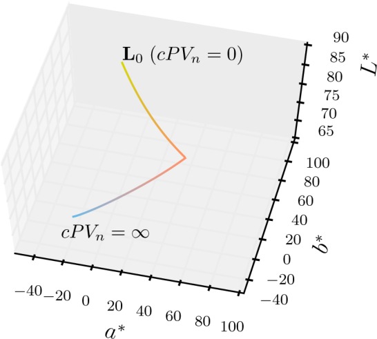
Color change trajectory in L^*a^*b^* color space according to cumulative polarization variance cPV.

The transformation T[] translate color in L^*a^*b^* color space to RGB color space by (1) converting the L^*a^*b^* color space into the XYZ color space [54], (2) applying a chromatic adaptation (using Bradford transform) from the D50 to D65 white points [55], and (3) converting XYZ color space to the linear sRGB space [56]. The resulting E is scaled by fitting the range [5, 99.9] percentile of the average RGB value, (R + G + B)/3, to within the range of [0, 1]. As this is in the linear sRGB space, the gamma correction is applied to fit with the sRGB standard [56]. We choose the sRGB color space because it is commonly used in Windows® operating system.

Note that we refer the “isolum” color map [57] to design m, L₀, and W[].

6. Results

JM-OCT described in elsewhere [49] is used to scan human eyes. The sampling configuration of JM-OCT is the same as previous, with 512 axial lines per frame acquired and the scan repeated four times at the same location (F = 4). The set of frames is scanned at 256 locations to construct a 3D volume set. The scanning speed is 100,000 lines/s, and the time lag between consecutive frames is 6.4 ms. JM-OCT simultaneously measures four complex OCT signals that correspond to four polarization channels (P = 4). For every cmOCA calculation, spatial kernel sizes are fixed to be (L = 3, D = 3) along the x and z directions, respectively. For scattering OCT image, global-phase-corrected sensitivity enhanced imaging with 4 frames followed by the coherently composition of 4 polarization-channel signals are applied [49].

All protocols for measurement were approved by the Institutional Review Board of the University of Tsukuba. Written, informed consent was obtained prior to measurement.

6.1. Complex correlation with/without SNR correction

The SNR-independent vasculature images can be obtained using our signal correlation estimator. Figure 4 shows a comparison of SNR-independent and -dependent cmOCAs. A cross section of the retina of a volunteer’s (male, 35 years old) right eye which had no remarkable abnormalities was obtained [Fig. 4(a)], and two correlation images were calculated. The SNR-independent and -dependent cmOCAs are obtained by mapping the magnitude of the signal correlation coefficient [Eq. (34)] and data correlation coefficient, which is estimated similar to Eq. (34) using ${\overline{r}}_G^{\mathrm{M}}$ as ${\overline{r}}_{Gf}^{\mathrm{M}}(x,Z)\equiv {\overline{r}}_G^{\mathrm{M}}(x,Z)/{\hat{r}}_m^{\mathrm{M}}(x)$. With the estimated data correlation ${\overline{r}}_{Gf}^{\mathrm{M}}$, both the perfused tissue and low-SNR region exhibit a low correlation, as with other correlation-based and phase-shift-based angiography methods [Fig. 4(b)]. With the signal correlation ${\overline{r}}_{Sf}^{\mathrm{M}}$, SNR-independent imaging is achieved [Fig. 4(c)]. Even the SNR of OCT signal at some non-perfused tissue, such as nuclear layers and vitreous humor, is low, its corresponding correlation coefficient exhibits close to 1. The presented cmOCA with SNR-corrected correlation distinguishes perfused tissues from low-SNR regions without the use of an arbitrary masking threshold.

Fig. 4.

Cross sections of the human retina. (a) Coherence composite OCT intensity, (b) SNR-dependent cmOCA, (c) SNR-independent cmOCA. The scale bar indicates 200 μm.

6.2. Comparison between single-channel and multi-channel implementations

For comparison, the correlation mapping method for the single-channel case [Eq. (29)] was applied to the complex summed OCT signal using the coherent composition [49]. The coherent composite signal clearly has a higher SNR than that of each channel, because the four polarization channels are coherently averaged. The correlation image is created with the coherent composite signal (Section 4.2.1).

Although the coherent composite signal has a higher SNR, the single-channel implementation exhibits significant spurious noise [Fig. 5(a)]. The images shows the left eye of a age-related macular degeneration patient (male, 79 years old) with the scanning range of 4.5 × 4.5 mm². When the SNR is low, the correlation between measured data ρ_G is low and the correlation estimation exhibits high variance. In addition, the large bias correction for estimating the signal correlation ρ_S enhances its variance.

Fig. 5.

Complex correlation mapping image of the human retina. cmOCA (b, d) with multiple polarization channels, as described in Section 4.2, exhibits lower spurious noise than (a, c) single-channel estimation with a coherent composite signal. The cross sections (a, b) and en-face slices (c, d) are taken from the locations indicated by the black arrows. Both cmOCAs used the same kernel size.

In contrast, the multi-channel method exhibits high contrast and low noise vessel imaging owing to the averaging process [Fig. 5(b)]. The corresponding en-face slice [Fig. 5(d)] visualizes the fine abnormal vascular network better than the single-channel method [Fig. 5(c)]. This shows that the second-step averaging is preferred for high-contrast vasculature imaging.

6.3. Motion artifact compensation

The performance of bulk-motion-artifact removal and bulk-phase-offset correction was evaluated with in vivo human posterior eye imaging. The left eye of a healthy subject (male, 27 years old) was scanned (6 × 6 mm²). Figure 6 illustrates the effect of bulk-motion-artifact removal (Section 3.2), and compares bulk-phase-offset correction using the new correlation-based estimation method (Section 3.1.1) against that with the complex-mean estimation method [46].

Fig. 6.

cmOCA cross sections without (a, b) and with (c, d) bulk-motion artifact removal. Bulk-phase-offset correction has been applied using the complex-mean method (a, c) and correlation-based method (b, d). The corresponding en-face projection images are shown in (e)–(h).

There is a thick blood vessel along the B-scan direction. With the previous average-based bulk-phase-offset estimation, the tissue above the thick blood vessel also has a low correlation coefficient [Fig. 6(a)]. This is because the erroneous average-based bulk-phase-offset estimation results in an incorrect phase-offset correction, and the phase-offset fluctuation between B-scan pairs reduces the correlation coefficient. Hence, applying the bulk-motion artifact removal with the average-based phase-offset correction over-corrects the correlation coefficient [Fig. 6(c)]. This effect reduces the contrast of thick blood vessels, as shown in Fig. 6(g) (yellow arrows).

With the new correlation-based phase-offset estimation method, the solid tissue exhibits a high correlation coefficient as expected [Fig. 6(b)]. The bulk-motion artifacts over the thick vessels are reduced. On the other hand, a small vessel overlaid on the thick vessel is retained (blue arrows), and the contrast of thick blood vessels in the en-face image is maintained well [Fig. 6(f), yellow arrows].

By applying bulk-motion artifact removal [Figs. 6(g) and (f)], artifacts appear as horizontal lines because the frame-by-frame bulk-motion decorrelation changes are well suppressed (green circles).

6.4. High-stability mode

In some cases, the phase of the swept-source OCT signal cannot be stabilized without a k-clock. The algorithm of Section 4.2 results in significant artifacts. In this case, high phase-noise-immunity mode (Section 3.1.2) can be applied. The details of the implementation is described in Appendix A.

A subject (male, 33 years old, right eye) was scanned (6 × 6 mm²) using JM-OCT, which has an unstable phase. As shown in Figs. 7(a) and 7(d), there are several artifacts that disturb the vasculature image. Using the correlation calculation in Eq. (44), these artifacts are significantly reduced, as shown in Figs. 7(b) and 7(e). Although the range of correlation has decreased to [0.3, 1.0], the contrast in the en-face projection is significantly improved. After motion artifact correction [Eq. (45)], horizontal line artifacts are suppressed (Fig. 7(f)). The high phase-noise-immunity mode is an alternative high-contrast vasculature imaging method for unstable phase systems.

Fig. 7.

cmOCA images with low-phase-stability SS-OCT system. The images were obtained using (a, d) the multichannel cmOCA algorithm (Section 4.2), (b, e) high phase-noise-immunity mode [Eq. (44)], and (c, f) high phase-noise-immunity mode with bulk-motion-artifact removal [Eq. (45)]. Cross sections (a, b, c) at the location indicated by the black arrow and en-face projections (d, e, f) are shown.

6.5. Retinal capillary imaging

To show the performance of the retinal capillary imaging with the cmOCA method, the same data set of Section 6.1 is used. The retinal layers are segmented to visualize the capillary network of different retinal layers. The Iowa Reference Algorithms (Retinal Image Analysis Lab, Iowa Institute for Biomedical Imaging, Iowa City, IA) [58–60] were applied to the coherent composite OCT intensity volume. The segmentation results were overlaid on a cross-sectional cmOCA image [Fig. 8(a)]. The en-face projection images of cmOCA volume visualize the retinal capillary vasculature at the fovea. From the anterior part, the retinal nerve fiber layer (NFL) + ganglion cell layer (GCL) [Fig. 8(b)], inner plexiform and nuclear layers (IPL + INL) [Figs. 8(c)], outer plexiform and nuclear layers (OPL + ONL) [8(d)] are shown.

Fig. 8.

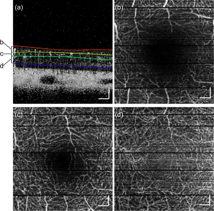
cmOCAs at the human fovea, (a) cross-sectional cmOCA image with segmented results, en-face projection images at (b) NFL + GCL, (c) IPL + INL, (d) OPL + ONL. The scanning area is 3 × 3 mm². The scale bar indicates 200 μm.

6.6. Eye disease case

A polypoidal choroidal vasculopathy (PCV) (female, 67 years old, left eye) is shown in Fig. 9. The composite projection image [Fig. 9(b)] combines the correlation mapping and DOPU data [53]. Details of the method are described in Section 5.3. This imaging method reveals whether vessels are covered or uncovered by multiple-scattering tissues, i.e., melanin. The orange-yellow color indicates that blood flow signals are unblocked (UB) by mDOPU signals (vasculature is in front of the pigmented tissues), whereas magenta-blue indicates that the flow signals are blocked (B). The cross-sectional image of the combination of OCT intensity (coherent composite + sensitivity-enhancement with global phase correction) and cmOCA reveals the relationship between morphology and vasculature. The log-scaled OCT intensity and cmOCA are assigned as blue and orange, respectively [57].

Fig. 9.

cmOCA images of polypoidal choroidal vasculopathy. En-face (a) OCT, (b) composition of cmOCA and mDOPU projection images. The scanning area is 6 × 6 mm². The corresponding area is indicated by the yellow rectangle in fluorescein angiography (c). The cross-sectional (d) OCT + cmOCA and (e) mDOPU images at the center of the scan [yellow line in (b)] are shown. The scale bar indicates 500 μm.

An abnormal blood flow signal can be observed in the cross section [Fig. 9(d), white circle]. The DOPU image [53] reveals some RPE detachment and its discontinuity [Fig. 9(e), white circle]. The corresponding signal appears in orange in the en-face composite projection image. This shows that the blood flow signal is not blocked by pigmented tissue, i.e., the RPE. The corresponding location exhibits hyperfluorescence in late-phase fluorescein angiography (FA) [Fig. 9(c)]. The composite imaging may be a good non-invasive alternative to FA for detecting the collocation of abnormal vessels with RPE disruption, such as choroidal neovascularization. Note that no segmentation is applied to generate the composite image, and so no segmentation errors are present.

7. Discussion

We have presented a method for estimating the SNR-corrected complex correlation coefficient with low noise. To compare the statistical properties of estimators, a numerical simulation was applied. A pair of random numbers X_i and X_i+1 in consecutive sets (i-th and i + 1-th sets) was generated by using the method to generate correlated random numbers. Outcomes Z_i and Y_i of independent complex Gaussian variables with zero mean and standard deviation σY were generated. Then, Y_i+1 was generated with the true correlation coefficient ρ as Y_i+1 = ρY_i + $\sqrt{1-{\rho }^2}$Z_i. Y_i and Y_i+1 will be correlated with the correlation coefficient ρ. Another outcome N_i of independent complex Gaussian variable with zero mean and standard deviation σ_N was generated and added to provide X_i = Y_i + N_i. By changing the ratio σ_Y/σ_N, arbitrary true SNR can be simulated. These generated signals X were processed with correlation estimators. For each trial, 4 sets of complex random Gaussian variable which have 9 sampling points were generated. The random number generation iterated four times to simulate 4 channels of JM-OCT. The data size for correlation estimate was 3 pairs from 4 sets of 9 data points times 4 channels, which is similar to the experiments. The mean and the standard deviation of estimates are obtained with 10,000 trials. The true correlation coefficient ρ was set to be 0.99, 0.9, and 0.8. The SNR 10log₁₀ ${\sigma }_Y^2/{\sigma }_N^2$ was set from 0 to 20 dB in 1 dB step.

Figure 10 shows the comparison of correlation estimates. The previous method with coherent composite and the new estimators give lower bias estimates than the normal data correlation estimate for every true correlation coefficient [Fig. 10(a), (b), and (c)]. At low SNR, the estimate with coherent composite exhibits lower bias than that of the new estimator. This is reasonable because the coherent composite decreases the noise. However, the standard deviation at high SNR is larger than that of the new estimator. This is because of the absence of the second averaging ${\langle \rangle }_{w_2}$. The advantage of the new estimator becomes greater as signal correlation decreases. It means that the imaging noise of blood vessels (where signal correlation is decreased) is lower in the case of the new estimator. Hence, the new estimation scheme is probably a good compromise in the sense of both bias and noise. This fact suggests that although SNR will be decreased, applying second averaging ${\langle \rangle }_{w_2}$ by splitting the OCT signal, such as spectrally splitting method [23], may provide better vasculature imaging with standard single channel OCT system at the same averaging kernel size.

Fig. 10.

The numerical simulation results of correlation coefficient estimates. (a, b, c) Mean and (d, e, f) standard deviation of each correlation estimator, i.e., data correlation (×), signal correlation with previous method using coherent composite (▲), and the new method (●) are plotted with several SNR. The set correlation coefficients are (a, d) 0.99, (b, e) 0.9, and (c, f) 0.8.

In our method, we introduced the sign function ε [Eq. (17)] in the denominator of the noise-corrected correlation estimate [Eq. (16)]. Although the absolute operation is applied inside the square root to avoid non-real-valued results in Eq. (16), the proposed estimator retains the sign ε after the noise correction. This modification from the previous method [29, 40] reduces the spurious appearance in the no signal region after second-step averaging ${\langle \rangle }_{w_2}$.

In the SNR range used in the abovementioned simulation, the sign ε in Eq. (16) does not affect to the estimator’s performance. The difference of the existence of ε becomes apparent at low SNR. The distributions of estimates with 0 SNR (−∞ dB) are shown in Fig. 11. The estimation is regarded as invalid if the estimated correlation is smaller than 0 or larger than 1. Because of the sign ε, the correlation estimates at 0 SNR spread and are less likely to be fall in the range of valid correlation coefficient estimate [0, 1]. With the sign ε, that probability of correlation estimate in the range [0, 1] occurs roughly 2.7 % [Fig. 11(c)], while this is 32.0 % in the case without ε [Fig. 11(a)] and 23.9 % in the case with thresholding [Fig. 11(b)]. Without the second averaging ${\langle \rangle }_{w_2}$, the thresholding method and the method using the sign ε provide the same probability. However, the second averaging generates a bias in the denominator of correlation coefficient estimate. This results in the large discrepancy after the second averaging.

Fig. 11.

Comparison of statistical properties at no signal region. Histograms of correlation estimates (a) without the sign ε, (b) without the sign ε and thresholding at 0 instead of absolute operation, and (c) with the sign ε Eq. (16) are shown. The numerical simulation of correlation estimates was applied at SNR=0.

8. Conclusion

Non-invasive vasculature imaging has been applied using complex-correlation-mapping OCA. Using low-bias and low-noise complex correlation estimation and motion artifact corrections, we have obtained better discrimination of perfusing tissue. The combination of perfusion contrast and polarization contrast demonstrates the potential of clinical utility in ophthalmology.

Appendix A. High-stability mode implementation

To implement the phase-noise-immune estimate (Section 3.1.2), no lateral and frame averaging is used to estimate the covariance matrix [Eq. (24)] because both depend on time in the system with scanning beam. Instead, polarization channel and axial averaging are used.

The correlation coefficient in the absence of phase noise is then obtained by substituting the averaging operators and noise power as shown in Table 4 into Eq. (18) as

$${\overline{r}}_S^{\sum }\left(\tau ;x,z\right)\equiv \frac{{\sum }_{l,f}^{L,F-1}\left|\frac{1}{D}{\sum }_{p,d}^{P,D}g(x+l,z+d,f,p)g*(x+l,z+d,f+1,p)\right|}{\begin{array}{r}{\sum }_{l,f}^{L,F-1}\epsilon (\tau ;x+l,z,f)\{|\left[\frac{1}{D}{\sum }_{p,d}^{P,D}{\left|g(x+l,z+d,f,p)\right|}^2-{\sum }_p^P{\hat{q}}_N(p)\right]\\ \times {\left[\frac{1}{D}{\sum }_{p,d}^{P,D}{\left|g(x+l,z+d,f+1,p)\right|}^2-{\sum }_p^P{\hat{q}}_N(p)\right]|\}}^{\frac{1}{2}}\end{array}}.$$ (44)

Table 4.

Assignment of averaging and variables of phase-noise-immune mode.

		High-stability mode (Section Appendix A)
Covariance matrix estimate	${\langle \cdot \rangle }_{w_1}$	$\frac{1}{DP}{\displaystyle \sum _{d,p}^{D,P}\cdot (z+d;p)}$
Correlation estimate	${\langle \cdot \rangle }_{w_2}$	$\frac{1}{(F-1)L}{\displaystyle \sum _{f,l}^{F-1,L}\cdot (f,f+1;x+l)}$
Noise power	${\hat{q}}_N$	$\frac{1}{P}{\displaystyle \sum _p^P{\hat{q}}_N(p)}$

The bulk-motion-artifact correction (Section 3.2) is then applied to ${\overline{r}}_S^{\sum }$(τ;x,z). For this correction, the phase-noise-immune data-correlation-coefficient ${\overline{r}}_G^{\sum }$(τ;x,z) is estimated using Eq. (44) without noise subtraction and ε. The net bulk-motion-induced phase-noise-immune data-correlation is estimated using Eq. (28) with ${\overline{r}}_G^{\sum }$(τ;x,z) as ${\overline{r}}_m^{\sum }$(τ;x) ≡ ${\overline{r}}_S^{\sum }(\tau ;x,\underset{z}{\arg \max }{\overline{r}}_G^{\sum }(\tau ;x,z))$. The bulk-motion-corrected phase-noise-immune signal correlation coefficient is finally estimated as

$${\overline{r}}_{Sf}^{\sum }(\tau ;x,z)\equiv \frac{{\overline{r}}_S^{\sum }(\tau ;x,z)}{{\hat{r}}_m^{\sum }(\tau ;x,)}.$$ (45)

Appendix B. List of notations

Symbols	Descriptions
G	complex random variable represents OCT data
S	complex random variable represents OCT signal
N	complex random variable represents additive noise
g	realization of OCT measurement
ΣG	population covariance matrix of OCT data
SG	sample covariance matrix of OCT data
sGpq	entries of SG
${\hat{q}}_N$	estimate of variance of noise N
ρG	population correlation coefficient of OCT data
ρS	population correlation coefficient of OCT signals
ρSNR	population de-correlation factor of OCT signals due to additive noise ρG/ρS
rG	sample correlation coefficient of OCT data
rS	sample correlation coefficient of OCT signal
${\overline{r}}_G$	estimate of data correlation coefficient
${\overline{r}}_S$	estimate of signal correlation coefficient
SNR	signal-to-noise ratio of OCT system E $\left[{\left|S\right|}^2\right]/\mathrm{E}\left[{\left|N\right|}^2\right]$
Δϕm	estimate of bulk-phase-offset
rm	decorrelation factor due to bulk motion
${\hat{r}}_m$	estimate of decorrelation factor rm
${\tilde{r}}_f$	net decorrelation due to flow
${\overline{r}}_{Sf}$	estimate of signal correlation coefficient after bulk-motion artifact removal
p	index of polarization channel (1,2,⋯,P)
f	index of frame (1,2,⋯,F)
D	averaging window size along axial direction
L	averaging window size along lateral direction