On Random Walks and Entropy in Diffusion-Weighted Magnetic Resonance Imaging Studies of Neural Tissue

Abstract

Purpose

In diffusion-weighted MRI studies of neural tissue, the classical model assumes the statistical mechanics of Brownian motion and predicts a monoexponential signal decay. However, there have been numerous reports of signal decays that are not monoexponential, particularly in the white matter.

Theory

We modeled diffusion in neural tissue from the perspective of the continuous time random walk. The characteristic diffusion decay is represented by the Mittag-Leffler function, which relaxes a priori assumptions about the governing statistics. We then used entropy as a measure of the anomalous features for the characteristic function.

Methods

Diffusion-weighted MRI experiments were performed on a fixed rat brain using an imaging spectrometer at 17.6 T with b-values arrayed up to 25,000 s/mm². Additionally, we examined the impact of varying either the gradient strength, q, or mixing time, Δ, on the observed diffusion dynamics.

Results

In white and gray matter regions, the Mittag-Leffler and entropy parameters demonstrated new information regarding subdiffusion and produced different image contrast from that of the classical diffusion coefficient. The choice of weighting on q and Δ produced different image contrast within the regions of interest.

Conclusion

We propose these parameters have the potential as biomarkers for morphology in neural tissue.

INTRODUCTION

The central feature of Brownian motion is that the mean squared displacement (MSD) grows linearly with time, 〈x²(t)〉 ~ t. However, three conditions must be satisfied: (1) the increments are normally distributed with zero mean, (2) the increments are independent (i.e., no memory), and (3) the process is continuous with an initial starting value set to zero (1). When any of these conditions are not met, the diffusion process is called anomalous and the MSD grows as a power law, 〈x²(t)〉 ~ t^γ (2). When γ > 1, the diffusion process is “superdiffusive” and when 0 < γ < 1, the diffusion process is “subdiffusive”. For Brownian motion, the characteristic function is represented by a monoexponential decay process with respect to time. In diffusion MRI studies, this is modeled as exp[−(bD)], where D is the diffusion coefficient (mm²/s) and b is a pulse sequence controlled parameter (3). However, numerous research groups have reported diffusion decay processes that deviate from the monoexponential model (4–11).

The random walk (RW) model is a practical approach to derive the features of Brownian motion. In the RW model, the random walker’s motion is governed by two stochastic processes: jump length distance, Δx, and waiting time (between jump lengths), Δt. When these incremental processes are governed by a finite characteristic waiting time and jump length variance, in the continuum limit as Δx → 0 and Δt → 0, the diffusion equation naturally arises (i.e., Fick’s second law) (12). A generalization to the RW model is the continuous time RW (CTRW) model in which the incremental processes are no longer constrained by a Gaussian or Poissonian probability distribution function (pdf). Rather, the jump lengths and waiting times are governed by arbitrary and independent pdfs (12,13). In the most general case, the random walker’s motion is represented with fractional powers α and β on the waiting time and jump length intervals, respectively, such that the MSD can be represented as a power law,

$$\langle x^2(t)\rangle ~t^{2\mathrm{\alpha }/\mathrm{\beta }},$$ [1]

where 0 < α ≤ 1 and 0 < β ≤ 2. When 2α/β = 1, the process is normal diffusion. When 2α/β > 1, the process is “superdiffusion”. When 0 < 2α/β < 1, the process is “subdiffusion”. Solving the CTRW in the continuum limit yields a characteristic decay process that is represented by the Mittag-Leffler function (MLF) (14). The MLF model is attractive in that it relaxes a priori assumptions about the governing statistics of the diffusion process.

In this report, we describe diffusion using the MLF (via α and β) and quantify the uncertainty of the CTRW using entropy for a diffusion-weighted MRI study on a healthy, fixed rat brain. Furthermore, we investigate the effects of weighting either q (i.e., gradient strength spatial resolution) and Δ (i.e., mixing time) on the data collected in diffusion MRI experiments. Finally, we measure the amount of “information” gained about biological tissue features, when the diffusion decay process is modeled with a decay function that is not monoexponential.

THEORY

From RWs to CTRWs

In the context of RW theory in which the jump length variances and characteristic waiting times are finite, the one-dimensional Brownian motion of a diffusing particle, P(x, t), in homogeneous and isotropic geometries can be described according to the second-order partial differential equation,

$$\frac{\partial P(x,t)}{\partial t}=D\frac{{\partial }^{2}P(x,t)}{\partial {\left|x\right|}^2},$$ [2]

where D is the diffusion coefficient. The solution to Eq. [2] follows as the familiar Gaussian form,

$$P(x,t)=\frac{1}{\sqrt{4\mathrm{\pi }Dt}}\exp \left(-\frac{x^2}{4Dt}\right).$$ [3]

However, in the context of CTRW theory in which the jump length variances and characteristic waiting times follow asymptotic power law distributions, the one-dimensional anomalous motion of a diffusing particle, P(x, t), in heterogeneous biological tissues characterized by tortuous and porous geometries, can be described with a fractional partial differential equation of the form,

$${ }_0^C{\mathcal{D}}_t^{\mathrm{\alpha }}(P(x,t))=D_{\mathrm{\alpha },\mathrm{\beta }}\frac{{\partial }^{\mathrm{\beta }}P(x,t)}{\partial {\left|x\right|}^{\mathrm{\beta }}},$$ [4]

where ${ }_0^C{\mathcal{D}}_t^{\mathrm{\alpha }}$ is the α^th (0 < α ≤ 1) fractional order time derivative in the Caputo form, ∂^β/∂|x|^β is the β^th (0 < β ≤ 2) fractional order space derivative in the Reisz form, and D_α,β is the effective diffusion coefficient (e.g., mm^β/s^α). The closed form solution of Eq. [4] can be given in the Fox’s H function,

$$P(x,t)=\frac{1}{\mathrm{\beta }\left|x\right|}{H}_{3,3}^{2,1}\left[\frac{-\left|x\right|}{D_{\mathrm{\alpha },\mathrm{\beta }}^{\frac{1}{\mathrm{\beta }}}{t}^{\frac{\mathrm{\alpha }}{\mathrm{\beta }}}}|\begin{array}{ccc}(1,\frac{1}{\mathrm{\beta }})& (\mathrm{\alpha },\frac{\mathrm{\alpha }}{\mathrm{\beta }})& (1,\frac{1}{2})\\ (1,1)& (1,\frac{1}{\mathrm{\beta }})& (1,\frac{1}{2})\end{array}\right].$$ [5]

When α = 1 and β = 2, Eq. [5] collapses to the Gaussian form in Eq. [3] (for proof see Ref. 15). However, the solution to Eq. [4] can be more succinctly written by performing a Fourier transform in space (P(x, t) → p(k, t)) to obtain the characteristic function,

$$p(k,t)=E_{\alpha }\left(-D_{\mathrm{\alpha },\mathrm{\beta }}{\left|k\right|}^{\mathrm{\beta }}{t}^{\mathrm{\alpha }}\right),$$ [6]

where E_α is the single-parameter MLF. The MLF is a well-behaved function defined as a power series expansion,

$$f(z)=E_{\mathrm{\alpha }}(z)={\displaystyle \sum _{k=1}^{\infty }\frac{{\left(z\right)}^k}{\mathrm{\Gamma }\left(\mathrm{\alpha }k+1\right)}},$$ [7]

where the Γ function is the generalized form of the factorial function, defined for real numbers (16). When α = 1 and β = 2, Eq. [6] collapses to an exponential function in the Gaussian form with respect to k,

$$p(k,t)=\exp (-D_{1,2}{\left|k\right|}^{2}t).$$ [8]

When α = 1 and 0 < β < 2, Eq. [6] returns a stretched exponential function with respect to k,

$$p(k,t)=\exp (-D_{1,\mathrm{\beta }}{\left|k\right|}^{\mathrm{\beta }}t).$$ [9]

When 0 < α < 1 and β = 2, Eq. [6] returns a stretched MLF with respect to t,

$$p(k,t)=E_{\mathrm{\alpha }}(-D_{\mathrm{\alpha },2}{\left|k\right|}^2{t}^{\mathrm{\alpha }}).$$ [10]

In the most general case of the solution to the diffusion equation shown in Eq. [6], the effective diffusion coefficient, D_α,β, has units of space^β/time^α. To formulate Eq. [6] such that the diffusion coefficient can be written as D_1,2 with units of space²/time, we insert parameters μ (space) and τ (time) to give,

$$p(k,t)=E_{\mathrm{\alpha }}\left(-D_{1,2}\frac{{\mathrm{\tau }}^{1-\mathrm{\alpha }}}{{\mathrm{\mu }}^{2-\mathrm{\beta }}}{\left|k\right|}^{\mathrm{\beta }}{t}^{\mathrm{\alpha }}\right),$$ [11]

such that,

$$D_{\mathrm{\alpha },\mathrm{\beta }}=D_{1,2}\frac{{\mathrm{\tau }}^{1-\mathrm{\alpha }}}{{\mathrm{\mu }}^{2-\mathrm{\beta }}}.$$ [12]

As α → 1 and β → 2, the term (τ^1−α/μ^2−β) → 1, and, that is to show Eq. [11] returns the Gaussian form in Eq. [8]. The parameters, μ and τ, are needed as an empirical solution to preserve the units for the diffusion coefficient, however, others have derived analogs to these parameters (i.e., Δx, Δt) in conservation of mass problems and heavy tailed limit convergence of fractal and fractional dynamics (14,17–19).

A phase diagram of α and β can be constructed to visualize the regions of subdiffusion, superdiffusion, and normal diffusion processes as shown in Figure 1. Moving leftward from the point of Gaussian diffusion (α = 1, and β = 2) by fixing α = 1 and decreasing β, the characteristic form of superdiffusion is given by Eq. [9] as a stretched exponential function. Moving downward from the point of Gaussian diffusion (α = 1, and β = 2) by fixing β = 2 and decreasing α the characteristic form of subdiffusion is given by Eq. [10] as a stretched MLF. For all other points inside the area bounded by the α = 1 horizontal and β = 2 vertical lines, the characteristic form of anomalous diffusion is given by Eq. [11]. The 2α/β = 1 diagonal represents effective normal diffusion in which the 〈x²(t)〉 ~ t, however, α and β are fractional and the non-Gaussian waiting time and jump length pdfs vie for competition of the mean-squared trajectory (20).

FIG. 1.

Anomalous diffusion phase diagram with respect to the order of the fractional derivative in space, β, and the order of the fractional derivative in time, α. (Adapted from Refs. 12 and 20)

From CTRW to Diffusion-Weighted MRI

In spin-echo diffusion MRI experiments, the signal decay, S, is modeled with a monoexponential as,

$$S/S_0=\exp (-bD),$$ [13]

where b is the product of the q-space and diffusion time terms, b = q²(Δ − δ/3) (3). For brevity, we will define $\overline{\mathrm{\Delta }}=\mathrm{\Delta }-\mathrm{\delta }/3$. As such, a diffusion-weighted experiment can be constructed with a set of b-values, with arbitrary weighting on the q and $\overline{\mathrm{\Delta }}$ components, so that a choice can be made to fix $\overline{\mathrm{\Delta }}$ and vary q in an array, or to fix q and vary $\overline{\mathrm{\Delta }}$ in an array.

In Ref. 21, a stretched exponential was fit to data obtained in fixed Δ, varying q experiments with a μ exponent and in fixed q, varying Δ experiments with an α exponent as an approach to independently interrogate fractional space and fractional time diffusion features described in Ref. 12, respectively. Additionally, in Ref. 11 temporal scaling effects were investigated in variable q and Δ experiments of a rat hippocampus by utilizing higher moment analysis of the propagator to find parameters, d_w and d_s, as fractal dimensions of the diffusion process and spectra, respectively. We expand on this previous work using the generalized solution to the diffusion equation from CTRW theory in Eqs. [6] and [11] to model anomalous diffusion in MRI as,

$$p(q,\overline{\mathrm{\Delta }})=E_{\mathrm{\alpha }}\left(-D_{1,2}\frac{{\mathrm{\tau }}^{1-\mathrm{\alpha }}}{{\mathrm{\mu }}^{2-\mathrm{\beta }}}{\left|q\right|}^{\mathrm{\beta }}{\overline{\mathrm{\Delta }}}^{\mathrm{\alpha }}\right),$$ [14]

where β absorbs the square of the q term to operate as 0 < β ≤ 2. With the perspective of the diffusion-weighted decay as the characteristic decay function, we also consider an entropy measure as a method to compare and contrast diffusion processes.

From Diffusion-Weighted MRI to Entropy in b-Space

In information theory, the amount of uncertainty in a discrete pdf, P(x) can be measured with,

$$H_x=-{\displaystyle \sum _{i=1}^{N}P(x_i)ln(P(x_i))},$$ [15]

where H_x is the Shannon information entropy (22). With the consideration of information formulated in the context of statistical uncertainty, we have a tool to compare systems governed by differing stochastic processes. For example, when comparing two α-stable distributions, the Gaussian and the Cauchy, normalized with the same full-width half maximum values, the Cauchy distribution can be shown to have greater information entropy. Non-Gaussian, or anomalous, diffusion phenomena have been correlated to regions of increased tissue complexity, like the white matter in the brain, which is relatively more anisotropic, heterogeneous, and tortuous compared with gray matter regions. From the information theory perspective, the white matter regions can be considered to have greater entropy than the gray matter regions, as they are governed by more uncertain diffusion pdfs.

Another approach to measure the uncertainty in a system is to analyze the characteristic function in terms of the Fourier transform in space (P(x) → p(k)) with spectral entropy,

$$H_k=-{\displaystyle \sum _{i=1}^N\frac{\widehat{p}(k_i)\ln (\widehat{p}(k_i))}{\ln (N)}},$$ [16]

where $\widehat{p}(k_i)=p(k_i)p^{\ast }(k_i)$ reflects the individual wavenumber’s contribution to a normalized power spectrum of the Fourier transform, p(k), and the term, ln(N) (i.e., discrete uniform distribution of N samples), is a normalization factor applied, so that the spectral entropy, H_k, is between 0 and 1 (23,24).

Furthermore, as Eq. [16] is generally defined to measure the uncertainty of a characteristic function, we can adapt this formalism for b-value diffusion decay signals as a function of q and $\overline{\mathrm{\Delta }}$,

$$H(q,\overline{\mathrm{\Delta }})=-{\displaystyle \sum _{i=1}^N\frac{\widehat{p}(q_i,\overline{\mathrm{\Delta }})\ln (\widehat{p}(q_i,\overline{\mathrm{\Delta }})}{\ln (N)}}.$$ [17]

By inserting the characteristic function in Eq. [14] (or, any definition of the characteristic function) into Eq. [17], the entropy in the diffusion process can be measured. For further analysis of entropy in anomalous diffusion processes, see Ref. 25.

METHODS

To evaluate the MLF parameters in Eq. [14] and the entropy, H(q, $\overline{\mathrm{\Delta }}$), defined in Eq. [17] as potential biomarkers for biological tissue features, we performed diffusion-weighted MRI measurements to investigate the effects of arraying q vs. arraying Δ on one healthy fixed rat brain. The outcomes of this pilot study will inform the experimental setup of an intersubject study on samples of healthy and neurodegenerative fixed rat brains. As the scope of this study is to investigate the effects of experimental setup on observed diffusion processes within the same biological tissue, one diffusion-weighted gradient direction was used. The y-axis diffusion weighting direction was chosen to evaluate the possibility of anomalous diffusion dynamics along the principal fiber direction of the corpus callosum, whereas other studies have reported anomalous diffusion in directions orthogonal to the principal fiber tracts (7,9). The effects of the diffusion weighting direction on the parameter values will be investigated in future studies to evaluate correlations to tensor metrics (e.g., first eigenvalue and fractional anisotropy).

The animal was prepared according to University of Florida’s Institutional Animal Care and Use Committee (UF IACUC protocol D710) (26). Overnight, prior to imaging experiments, the rat brain was soaked in phosphate-buffered saline. For the imaging experiment, the rat brain was placed in a 20-mm imaging tube, and the tube was filled with Fluorinert and secured with a magnetic susceptibility-matched plug to minimize vibrational movement due to the pulsed gradients. The rat brain was oriented in the spectrometer such that the anterior–posterior oriented along the main B0 field (z-axis), the superior–inferior with x-axis, and the lateral with the y-axis. At the Advanced Magnetic Resonance Imaging and Spectroscopy (AMRIS) Facility (Gainesville, FL), pulsed gradient stimulated echo diffusion-weighted experiments were performed on a Bruker spectrometer at 750 MHz (17.6 T, 89-mm bore) with the following parameters: pulse repetition time = 2 s, echo time = 28 ms, b-values up to 25,000 s/mm², δ = 3.5 ms, NA = 2, y-axis diffusion weighting, 1 central slice in the y–z plane, slice thickness = 1 mm, field of view = 27 × 18 mm², matrix size of 142 × 94 pixels, in-plane resolution of 190 μm. It should be highlighted that in all experiments, δ ≪ Δ to ensure the short-pulse approximation remained valid. Variable TR data (echo time = 12.5 ms, pulse repatition time = 300–3600 ms, increments of 300 ms) were collected to correct the pulse gradient stimulated echo data for T₁ relaxation effects. Additionally, the pulse gradient stimulated echo data were Rician noise corrected. See Appendix for data processing details.

Two constant Δ, variable q experiments were performed with Δ fixed at 17.5 and 50 ms. Two constant q, variable Δ experiments were performed with gradient strengths (g_y) at 350 and 525 mT/m to achieve q-values of 52 and 78 mm⁻¹, respectively. For the constant Δ = 17.5 ms experiment, q was arrayed at 0, 39.7, 55.5, 67.7, 95.4, 116.7, 134.7, 150.5, 164.9, 178.1, and 190.3 mm⁻¹. For the constant Δ = 50 ms experiment, q was arrayed at 0, 24.9, 33.8, 40.9, 57.0, 69.4, 79.9, 89.2, 97.7, 105.4, and 112.4 mm⁻¹. For the constant q = 78 mm⁻¹ experiment, Δ was arrayed at 17.5, 31.5, 45.5, 59.5, 73.5, 87.5, 101.5, 108.5, and 115 ms. For the constant q = 52 mm⁻¹ experiment, Δ was arrayed at 17.5, 51.5, 85.5, 119.5, 153.5, 187.5, 221.5, 238.5, and 250 ms.

Because the generalized diffusion model in Eq. [14] specifies D_1,2, μ, and τ as a ratio, any number of parameter value combinations can satisfy successful fitting results. To constrain these parameters, D_1,2, μ, and τ were first estimated using intermediate fits. To estimate the diffusion coefficient, a monoexponential function was fit to the first three low b-value samples, referred to as, D_m. After D_m estimation, two analogous stretched exponential fitting procedures were used to fit the constant $\overline{\mathrm{\Delta }}$ and constant q experimental data to find estimates of μ and τ, denoted as $\overline{\mathrm{\mu }}$ and $\overline{\mathrm{\tau }}$. The form of these stretched exponential functions utilize the diffusion experiment pulse sequence parameters to independently constrain the magnitudes of $\overline{\mathrm{\mu }}$ and $\overline{\mathrm{\tau }}$. The stretching parameters in these intermediate fits, $\overline{\mathrm{\alpha }}$ and $\overline{\mathrm{\beta }}$, were each placed over the entire b-value (Eqs. [A3], [A6], [A9], and [A12]), which differs from the stretching form of ${\overline{\mathrm{\Delta }}}^{\mathrm{\alpha }}$ and q^β in Eq. [14]. See Appendix for fitting details.

Following the intermediate parameter estimations, D_m, $\overline{\mathrm{\mu }}$, $\overline{\mathrm{\tau }}$, α = 1, and β = 2 were used as starting values in the nonlinear least squared fit of the MLF (www.mathworks.com/matlabcentral/fileexchange/8738) to converge on D_1,2, μ, τ, α, and β values. D_1,2, μ, and τ were allowed to float ±50% from their initial estimates. The value for α was bounded between 0 and 1.1 and β between 0 and 2.2. All fits were performed with a nonlinear least squares fitting algorithm in Matlab (Nantick, MA) in which the convergence criteria for the estimated coefficients was 10⁻⁶.

To challenge the robustness of the fitting routine to identify the diffusion regimes delineated on the phase diagram in Figure 1 via the MLF parameters, simulations were performed for known permutations of α and β in the presence of random noise added to decay signals. Signals were created for: space- and time-fractional Brownian motion (α = 0.5, and β = 1) of the form in Eq. [6], Brownian motion (α = 1, and β = 2) of the form in Eq. [8], space-fractional superdiffusion (α = 1, and β = 1) of the form in Eq. [9], and time-fractional subdiffusion (α = 0.5, and β = 2) of the form in Eq. [10]. The simulated random noise was modeled using the Rician noise profile measured from the diffusion experiments and gradually increased until either α or β diverged more than ±0.1 from their given values. For all simulated permutations of α and β, the estimated values were stable within ±0.1 from their given values (P < 0.05) when random noise was added up to three standard deviations larger than the experimental noise profile.

After the MLF parameters were determined, the characteristic decay curve for p(q, $\overline{\mathrm{\Delta }}$) was constructed using N = 1500 increments arrayed over variable q or variable $\overline{\mathrm{\Delta }}$ for b-values between 0 and 25,000 s/mm². Then, the entropy (defined in Eq. [17]) in the diffusion process, as modeled by the MLF, was computed as H(q, $\overline{\mathrm{\Delta }}$)_MLF. For comparison, using the monoexponential model (D_m) in Eq. [13], a characteristic decay curve of N = 1500 increments arrayed over b-values between 0 and 25,000 s/mm² was constructed. The entropy in the diffusion process, as modeled by the monoexponential function, was computed as H(q, $\overline{\mathrm{\Delta }}$)_mono.

RESULTS

Figure 2 shows a T₂-weighted image of an axial slice through a whole, healthy fixed rat brain with seven regions of interest (ROIs) in the cerebral cortex, striatum, and corpus callosum. These ROIs were selected to analyze tissue compositions ranging from gray matter (cerebral cortex), to a mixture of gray and white matter (striatum), and to white matter (corpus callosum). Furthermore, the y-axis diffusion weighting direction was selected to coincide with the principal fiber orientation of the central corpus callosum (ROI 4).

FIG. 2.

T₂-weighted image of an axial slice in a fixed rat brain with ROIs: left (1) and right (2) cerebral cortex; left (3), central (4), and right (5) corpus callosum; left (6) and right (7) striatum.

Figures 3–6 show the parameter maps for the MLF in Eq. [14] and the entropy in [17] in the four constant Δ₁ = 17.5 ms, Δ₂ = 50 ms, q₁ = 78 mm⁻¹, and q₂ = 52 mm⁻¹ experiments. For the seven ROIs, all numerical=values for the MLF parameters in the four experiments are available in the Supporting Information. The results for the MLF parameter maps are reported as the mean and standard deviation values for each ROI. In all experiments, α separated the cerebral cortex (ROIs 1 and 2), the central corpus callosum (ROI 4), and the striatum (ROIs 6 and 7). In the q₁ (Fig. 5) and q₂ (Fig. 6) experiments, α distinguished the central corpus callosum (ROI 4) from the lateral corpus callosum (ROIs 3 and 5). In all the experiments, β showed less contrast than α and for the regions containing gray matter, β → 2, indicating Gaussian statistics on the jump length distributions. However, in the Δ₁ (Fig. 3) and Δ₂ (Fig. 4) experiments, β separated the central corpus callosum from the regions containing gray matter (ROIs 1, 2, 6, and 7). In the Δ₁ and Δ₂ experiments, the diffusion coefficient, D_1,2, separated the central corpus callosum from the striatum (ROIs 6 and 7). In the q₁ experiment, μ separated the central corpus callosum from the regions containing gray matter (ROIs 1, 2, 6, and 7). In the Δ₁, Δ₂, and q₁ experiments, τ separated the central corpus callosum from the regions containing gray matter (ROIs 1, 2, 6, and 7). It should also be noted the mean values across the ROIs for μ and τ are different when fixing Δ and fixing q to the different values in the experiments. From the Δ₁ to the Δ₂ experiment, the mean μ scaled from ~2.3 to ~3.6 μm and the mean τ scaled from ~19.2 to ~57.1 ms. From the q₁ to the q₂ experiment, the mean μ scaled from ~2.1 to ~3.3 μm, and the mean τ scaled from ~24.1 to ~36.8 ms.

FIG. 3.

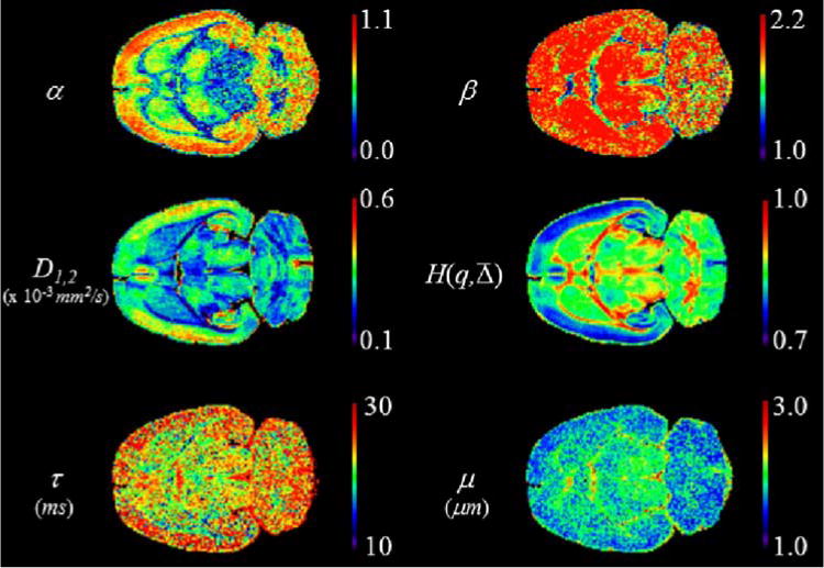
MLF and entropy parameter maps for constant Δ₁ = 17.5 ms experiment (y-axis diffusion weighting). [Color figure can be viewed in the online issue, which is available at wileyonlinelibrary.com.]

FIG. 6.

MLF and entropy parameter maps for constant q₂ = 52 mm⁻¹ experiment (y-axis diffusion weighting). [Color figure can be viewed in the online issue, which is available at wileyonlinelibrary.com.]

FIG. 5.

MLF and entropy parameter maps for constant q₁ = 78 mm⁻¹ experiment (y-axis diffusion weighting). [Color figure can be viewed in the online issue, which is available at wileyonlinelibrary.com.]

FIG. 4.

MLF and entropy parameter maps for constant Δ₂ = 50 ms experiment (y-axis diffusion weighting). [Color figure can be viewed in the online issue, which is available at wileyonlinelibrary.com.]

Table 1-a reports the entropy of the characteristic function as represented by the MLF. In the Δ₁, Δ₂, and q₁ experiments, H(q, $\overline{\mathrm{\Delta }}$)_MLF distinguished the central corpus callosum (ROI 4) from the lateral white matter (ROIs 3 and 5). In the Δ₁, Δ₂, and q₁ experiments, H(q, $\overline{\mathrm{\Delta }}$)_MLF separated the cerebral cortex (ROIs 1 and 2), the central corpus callosum (ROI 4), and the striatum (ROIs 6 and 7).

Table 1.

Entropy Values for the ROIs in the Constant Δ₁ = 17.5 ms, Δ₂ = 50 ms, q₁ = 78 mm⁻¹, and q₂ = 52 mm⁻¹ Experiments

Parameter	ROI	Δ1	Δ2	q1	q2
(a) H(q, Δ)MLF	(1) Cortex, l	0.82 ± 0.01	0.78 ± 0.01	0.78 ± 0.01	0.76 ± 0.01
	(2) Cortex, r	0.83 ± 0.01	0.81 ± 0.01	0.79 ± 0.01	0.78 ± 0.01
	(3) Corpus callosum, l	0.88 ± 0.02	0.85 ± 0.03	0.83 ± 0.02	0.80 ± 0.02
	(4) Corpus callosum, c	0.93 ± 0.01	0.91 ± 0.01	0.88 ± 0.02	0.83 ± 0.01
	(5) Corpus callosum, r	0.88 ± 0.02	0.86 ± 0.03	0.83 ± 0.02	0.81 ± 0.02
	(6) Striatum, l	0.86 ± 0.01	0.83 ± 0.01	0.82 ± 0.01	0.81 ± 0.01
	(7) Striatum, r	0.86 ± 0.01	0.83 ± 0.01	0.82 ± 0.01	0.81 ± 0.01
(b) H(q, Δ)mono	(1) Cortex, l	0.76 ± 0.01	0.75 ± 0.01	0.78 ± 0.01	0.77 ± 0.01
	(2) Cortex, r	0.77 ± 0.01	0.80 ± 0.01	0.79 ± 0.01	0.78 ± 0.01
	(3) Corpus callosum, l	0.76 ± 0.02	0.76 ± 0.04	0.80 ± 0.02	0.78 ± 0.02
	(4) Corpus callosum, c	0.74 ± 0.01	0.75 ± 0.02	0.81 ± 0.01	0.78 ± 0.01
	(5) Corpus callosum, r	0.76 ± 0.01	0.79 ± 0.02	0.80 ± 0.01	0.78 ± 0.01
	(6) Striatum, l	0.78 ± 0.01	0.78 ± 0.01	0.80 ± 0.01	0.79 ± 0.01
	(7) Striatum, r	0.78 ± 0.01	0.81 ± 0.01	0.80 ± 0.01	0.80 ± 0.01

Table 2 shows the ratio, 2α/β as the composite exponent in the context of the trajectory of the MSD as defined in Eq. [1]. In the Δ₁ experiment, all ROIs reported subdiffusion (2α/β < 1), with the lateral corpus callosum regions growing slowest with respect to time. In the Δ₂ experiment, the corpus callosum ROIs are most subdiffusive, whereas the cortex and striatum show slight subdiffusion and effective normal diffusion (2α/β → 1). In the q₁ experiment, the central corpus callosum ROI is most subdiffusive, whereas the cortex and striatum show slight subdiffusion and effective normal diffusion. In the q₂ experiment, the ROIs report a diminished range of slight subdiffusion and effective normal diffusion.

Table 2.

2α/β Composite Exponent for the ROIs in the Constant Δ₁ = 17.5 ms, Δ₂ = 50 ms, q₁ = 78 mm⁻¹, and q₂ = 52 mm⁻¹ Experiments

ROI	Δ1	Δ2	q1	q2
(1) Cortex, l	0.76 ± 0.08	0.98 ± 0.09	0.98 ± 0.02	1.00 ± 0.03
(2) Cortex, r	0.76 ± 0.08	0.92 ± 0.02	0.98 ± 0.03	0.99 ± 0.02
(3) Corpus callosum, l	0.45 ± 0.12	0.57 ± 0.30	0.86 ± 0.04	0.91 ± 0.03
(4) Corpus callosum, c	0.74 ± 0.12	0.54 ± 0.05	0.75 ± 0.05	0.84 ± 0.03
(5) Corpus callosum, r	0.37 ± 0.16	0.56 ± 0.17	0.87 ± 0.05	0.87 ± 0.04
(6) Striatum, l	0.62 ± 0.08	0.90 ± 0.13	0.90 ± 0.01	0.95 ± 0.03
(7) Striatum, r	0.58 ± 0.06	0.83 ± 0.03	0.91 ± 0.02	0.94 ± 0.03

DISCUSSION

In the classical monoexponential model when α is fixed at 1 and β at 2 in Eq. [8], the characteristic function is concisely written as Eq. [13], (i.e., exp(−bD)). Using entropy, it is possible to measure the amount of information contained in an ROI as the characteristic function deviates from a monoexponential decay. Table 1-b reports the entropy of the characteristic function as represented by the monoexponential. Across all of the experiments, H(q, $\overline{\mathrm{\Delta }}$)_mono is unable to distinguish between the ROIs. However, a comparison can be made to Table 1-a in which the MLF model is used to model the diffusion process. In the Δ₁ experiment, for example, the most information was learned about the diffusion process in the corpus callosum ROIs, followed by striatum, and cortex ROIs, respectively. It is interesting to note that the amount of information learned diminishes as the fixed diffusion time increases (i.e., from Δ₁ to Δ₂ experiment) and, inversely, as the fixed diffusion gradient strength decreases (i.e., from q₁ to q₂ experiment). Figure 7 shows the entropy maps for the MLF and monoexponential models with each experiment demonstrating the improved image contrast in H(q, $\overline{\mathrm{\Delta }}$)_MLF compared to H(q, $\overline{\mathrm{\Delta }}$)_mono. It should also be noted that D_m and D_1,2 were statistically indistinguishable (comparison table available in the Supporting Information), which indicates the diffusion coefficient units were preserved in the MLF fitting routine. Another way to visualize information contained in the characteristic function is simply to look at the diffusion decay signals in log-linear plots, for example, as shown in Figure 8. On this scale, a monoexponential decay would appear as a straight line, however, the cortex, striatum, and corpus callosum all deviate as the b-values increase. As the corpus callosum data are more anomalous than the striatum, and the striatum more anomalous than the cortex, corresponding information is added at high b-values to distinguish the ROIs. Figure 8 also shows the MLF curves to demonstrate the small mean squared error of the fits, which is representative for all data analyzed in this study.

FIG. 7.

Entropy parameter maps for the MLF (left) and monoexponential (right) fits of the characteristic function in the Δ₁ = 17.5 ms (row 1), Δ₂ = 50 ms (row 2), q₁ = 78 mm⁻¹ (row 3), and q₂ = 52 mm⁻¹ (row 4) experiments (y-axis diffusion weighting).

FIG. 8.

Signal decay plots and MLF fits for the cerebral cortex (ROI 1, circles), striatum (ROI 6, squares), and corpus callosum (ROI 4, triangles) in the Δ = 17.5 ms experiment (y-axis diffusion weighting).

In the context of CTRW theory, it is interesting to break down the composite exponent on the MSD trajectory, 2α/β, in the context of waiting time, jump length distributions, and entropy. In the continuum limit, the waiting time (Δt → 0) and jump length (Δx → 0) increments can be represented, in the most general case, as fractional time and space derivatives of arbitrary orders, α and β, respectively. As the order of the fractional derivatives move away from the special case of Brownian motion (α = 1, and β = 2), the waiting times and jump lengths are governed by heavy tailed distributions in which the diffusing particle has a greater probability of waiting longer and jumping further. So, the composite exponent on the MSD trajectory can take on a particular value to indicate subdiffusive growth, but can be comprised of different combinations of fractional values for α and β. For example, in the Δ₁ experiment, the composite exponents are similar for the right cerebral cortex (~0.76) and the central corpus callosum (~0.74), indicating subdiffusive growth. However, the individual values of α and β are clearly different for the right cerebral cortex (α ~ 0.74, and β ~ 1.95) and the central corpus callosum (α ~ 0.42, and β ~ 1.15). Therefore, the characteristic function representation for the waiting time and jump length distributions is more uncertain (anomalous) in the central corpus callosum compared to the right cerebral cortex. And, this difference is clearly encoded in the entropy with the corpus callosum (H(q, $\overline{\mathrm{\Delta }}$) ~ 0.93) and the cerebral cortex (H(q, $\overline{\mathrm{\Delta }}$) ~ 0.83). Increasing the diffusion time from the Δ₁ to the Δ₂ experiment, the composite exponent increased for all ROIs, except the central corpus callosum where 2α/β decreased from ~0.74 to ~0.54. Between these two experiments, there was no significant change in α, however β increased from ~1.15 to ~1.42 reflecting the smaller range of q-values sampled in the Δ₂ experiment to resolve the spatial component of the anomalous diffusion in this heterogenous and tortuous ROI.

The probabilistic framework of the CTRW theory models diffusion in any environment that has heterogeneous, tortuous, and multiscale properties (12,13,27–30). In this study, we have applied this abstract approach to the realm of biological tissues and MRI physics. However, work remains to correlate these new parameters to anatomical features as has been done to validate diffusion tensor imaging parameters with histology (31–33). It is encouraging to consider the results of this study in the context of high-resolution electron micrograph images of fixed mouse neural tissue reported in Ref. 34. These images show that although there is a principal fiber direction in the corpus callosum, within the resolution of one imaging voxel (~200 μm), there are also clearly visible populations of heterogeneous, tortuous, and crossing fibers, particularly in the central region. So, it is a reasonable hypothesis to propose the tissue microstructure is reflected in α as the likelihood for water to be “trapped” within a hindrance and β as the likelihood for water to “jump” along a less-hindered environment.

As the images in Figures 3–7 show, there is new contrast that is different from the diffusion coefficient map. Even where contrast is not as apparent (i.e., β, μ, and τ), there is information about the ROI and the experiment. When β → 2, the spatial component (i.e., jump length) of the diffusion dynamics approaches the form of a normal distribution. When raising the arguments, q and $\overline{\mathrm{\Delta }}$ to fractional powers, μ and τ are required to preserve the units of the diffusion coefficient, and the scales of their values are initially dependent on the diffusion experiment’s fixed component (q or Δ) in the b-value array, as described in the Appendix. As the fits for the signal decay data converge to fractional values for α and β, mathematically, the values for μ and τ are affected, and this was observed in the central corpus callosum for the Δ₁, Δ₂, and q₁ experiments, mentioned earlier. By dissecting and weighting a b-value with its controllable pulse sequence variables, μ and τ are reflective of both the experimental setup and the decay curve. The values for μ are scaled on the order of microns and, perhaps, are indicative of the subvoxel resolution in the diffusion experiment. Whereas the values for τ are scaled on the order of milliseconds and, perhaps, are indicative of the non-Markovity (i.e., memory) of the diffusion process as the longest times were observed in the central corpus callosum, along the principal fiber orientation.

It is difficult to compare the outcomes of this study with respect to other reports of anomalous diffusion modeled with a stretched exponential function. In Refs. 7–9, the stretching exponent is raised over the entire b-value (i.e., $(q^2\overline{\mathrm{\Delta }})$). In Refs. 5 and 6, the q² term is raised by a β parameter; however, there is no stretching term on $\overline{\mathrm{\Delta }}$ (i.e., α = 1), as the Bloch-Torrey equation was generalized solely with a fractional space derivative to arrive at the stretched exponential form. However, it is encouraging to note that the values (i.e., microns) estimated for μ in our study are similar to those reported in Refs. 5,6. In Ref. 21, stretching exponents were placed each on q² and $\overline{\mathrm{\Delta }}$, but were done so with individual fits in which one of the exponents was fixed at a time, whereas our approach ultimately produces a simultaneous estimation of the stretching exponents on q² and $\overline{\mathrm{\Delta }}$. In Ref. 11, numerous diffusion experiments were performed by manipulating the weightings of q and $\overline{\mathrm{\Delta }}$ to investigate temporal scaling of fractal measures by applying a q-space analysis in a rat hippocampus where subdiffusive power-law growth of the propagator is also reported.

Finally, it is apparent that how the experiment’s parameters are selected, by either arraying the gradient strength or the mixing time, and the weightings therein, affect the diffusion dynamics observed within an ROI. In the context of entropy (Table 1 and Fig. 7) as a measure of “uncertainty” in the diffusion decay signal, our study suggests that fixing Δ at the shortest time and arraying across a large range of q values produced the most “information” about the probed neural tissue in comparison to the three other experiments. That is to say, the experiment should minimize the diffusion time such that the water still has enough time to explore the environment, while the gradient strength is maximized to resolve the tissue microstructure within the imaging voxel. From this perspective, it is important that the diffusion experiment is tuned to match the neural tissue under study to observe dynamics, which may not be as clearly resolved if the mixing time or the diffusion gradient strength is not optimal.

CONCLUSIONS

In this study, we approached the diffusion decay signal in the probabilistic regime as a representation of the characteristic function—the Fourier transform of the pdf. In the context of CTRW theory, we examined the diffusion dynamics in terms of the waiting time and jump length distributions. For ROIs that are heterogenous and tortuous, like the corpus callosum, the representative parameters, α and β, showed deviations away from the Gaussian case of Brownian motion (α = 1, and β = 2) To quantify these deviations, we applied entropy as an overall measure of the anomalous nature of the diffusion process. At high b-values, new “information” was learned using a model (MLF) that is able to capture heavy-tailed diffusion signal decays that are not monoexponential. As such, the MLF and entropy parameters are potential biomarkers for degeneration, plasticity, therapeutic response in neural tissue. It is important to emphasize that the choice of q and Δ impacts the observed outcomes as demonstrated in each of the constant q and constant Δ experiments. Future studies will focus on control vs. disease models and histological correlation to these parameters. Additionally, the methods presented in this report will be adapted for human clinical systems, which have a smaller range of diffusion gradient strengths and mixing times. More advanced fitting algorithms will be investigated (e.g., simulated annealing, two-dimensional nonlinear regression) for use in conjunction with the MLF when assessing inter-subject variability. Finally, investigations are in progress to quantify the directional dependence of the CTRW parameters, and of the entropy, which can in principle—just as the diffusion coefficient—be described with tensor constructs.

APPENDIX: DATA PROCESSING

Raw Signal Corrections

For each voxel, the raw signal S_raw was Rician noise corrected with,

$$S_{\text{rc}}=\sqrt{S_{\text{raw}}^2-2{\mathrm{\sigma }}_{\mathrm{n}}^2,}$$ [A1]

where S_rc is the Rician corrected signal and ${\mathrm{\sigma }}_{\mathrm{n}}^2$ is the variance in the background noise floor.

To account for T₁ recovery effects at long diffusion times, S_rc was corrected with,

$$S=S_{\text{rc}}\exp (\mathrm{\Delta }/T_1),$$ [A2]

where T₁ was computed using the variable pulse repetition time data.

Constant Δ Experiment μ and τ Estimations

For the constant Δ, variable q experiments, first an estimate of μ was made followed by an estimate of τ. To estimate μ as $\overline{\mathrm{\mu }}$, the signal decay was fit to,

$$S/S_0=\exp [-{(b{D}_{\overline{\mathrm{\beta }}})}^{\overline{\mathrm{\beta }}}],$$ [A3]

where $D_{\overline{\mathrm{\beta }}}$ is the apparent diffusion coefficient of an exponential function stretched in $\overline{\mathrm{\beta }}$. Thus, it follows that a diffusion coefficient equivalency can be formulated as,

$${\left(D_{\overline{\mathrm{\beta }}}\right)}^{\overline{\mathrm{\beta }}}=D_{\mathrm{m}}{\left(\frac{\overline{\mathrm{\Delta }}}{{\overline{\mathrm{\mu }}}^2}\right)}^{1-\overline{\mathrm{\beta }}}$$ [A4]

to solve for $\overline{\mathrm{\mu }}$,

$$\overline{\mathrm{\mu }}=\sqrt{\overline{\mathrm{\Delta }}}{\left[\frac{{\left(D_{\overline{\mathrm{\beta }}}\right)}^{\overline{\mathrm{\beta }}}}{D_{\mathrm{m}}}\right]}^{\frac{1}{2(\overline{\mathrm{\beta }}-1)}},$$ [A5]

where the value for $\overline{\mathrm{\Delta }}$ is known from the constant Δ experiment. Then, to estimate τ as $\overline{\mathrm{\tau }}$, the signal decay was fit to,

$$S/S_0=\exp \left[-D_{\overline{\mathrm{\alpha }}}\frac{1}{{\overline{\mathrm{\mu }}}^2}{(b{\overline{\mathrm{\mu }}}^2)}^{\overline{\mathrm{\alpha }}}\right],$$ [A6]

where $D_{\overline{\mathrm{\alpha }}}$ is the apparent diffusion coefficient of an exponential function stretched in $\overline{\mathrm{\alpha }}$. Thus, it follows that a diffusion coefficient equivalency can be formulated as,

$$D_{\overline{\mathrm{\alpha }}}=D_{\mathrm{m}}\left(\frac{\overline{\mathrm{\Delta }}}{{\overline{\mathrm{\tau }}}^{\overline{\mathrm{\alpha }}}}\right)$$ [A7]

to solve for $\overline{\mathrm{\tau }}$,

$$\overline{\mathrm{\tau }}={\left(\overline{\mathrm{\Delta }}\frac{D_{\mathrm{m}}}{D_{\overline{\mathrm{\alpha }}}}\right)}^{\frac{1}{\overline{\mathrm{\alpha }}}},$$ [A8]

again, where the value for $\overline{\mathrm{\Delta }}$ is known from the constant Δ experiment.

Constant q Experiment μ and τ Estimations

For the constant q, variable Δ experiments, first an estimate of τ was made followed by an estimate of μ. To estimate τ as $\overline{\mathrm{\tau }}$, the signal decay was fit to,

$$S/S_0=\exp [-{\left(b{D}_{\overline{\mathrm{\alpha }}}\right)}^{\overline{\mathrm{\alpha }}}],$$ [A9]

where $D_{\overline{\mathrm{\alpha }}}$ is the apparent diffusion coefficient of an exponential function stretched in $\overline{\mathrm{\alpha }}$. Thus, it follows that a diffusion coefficient equivalency can be formulated as,

$${\left(D_{\overline{\mathrm{\alpha }}}\right)}^{\overline{\mathrm{\alpha }}}=D_{\mathrm{m}}{\left(q^2\overline{\mathrm{\tau }}\right)}^{1-\overline{\mathrm{\alpha }}}$$ [A10]

to solve for $\overline{\mathrm{\tau }}$,

$$\overline{\mathrm{\tau }}=\frac{1}{q^2}{\left[\frac{{\left(D_{\overline{\mathrm{\alpha }}}\right)}^{\overline{\mathrm{\alpha }}}}{D_{\mathrm{m}}}\right]}^{\frac{1}{1-\overline{\mathrm{\alpha }}}},$$ [A11]

where the value for q is known from the constant q experiment. Then, to estimate μ as $\overline{\mathrm{\mu }}$, the signal decay was fit to,

$$S/S_0=\exp \left[-D_{\overline{\mathrm{\beta }}}\overline{\mathrm{\tau }}{\left(\frac{b}{\overline{\mathrm{\tau }}}\right)}^{\overline{\mathrm{\beta }}}\right],$$ [A12]

where $D_{\overline{\mathrm{\beta }}}$ is the apparent diffusion coefficient of an exponential function stretched in $\overline{\mathrm{\beta }}$. Thus, it follows that a diffusion coefficient equivalency can be formulated as,

$$D_{\overline{\mathrm{\beta }}}=D_{\mathrm{m}}\left(\frac{{\mathrm{\mu }}^{\overline{\mathrm{\beta }}}}{q^2}\right)$$ [A13]

to solve for $\overline{\mathrm{\mu }}$,

$$\overline{\mathrm{\mu }}={\left(q^2\frac{D_{\overline{\mathrm{\beta }}}}{D_{\mathrm{m}}}\right)}^{\frac{1}{\overline{\mathrm{\beta }}}},$$ [A14]

again, where the value for q is known from the constant q experiment.

References

- 1.Mazo RM. Brownian motion: fluctuations, dynamics, and applications. Oxford, UK: Clarendon Press; 2009. [Google Scholar]
- 2.Cushman JH, O’Malley D, Park M. Anomalous diffusion as modeled by a nonstationary extension of Brownian motion. Phys Rev E: Stat Nonlin Soft Matter Phys. 2009;79:032101. doi: 10.1103/PhysRevE.79.032101. [DOI] [PubMed] [Google Scholar]
- 3.Le Bihan D. Diffusion and perfusion magnetic resonance imaging: applications to functional MRI. New York: Raven Press; 1995. [Google Scholar]
- 4.Bennett KM, Schmainda KM, Bennett RT, Rowe DB, Lu H, Hyde JS. Characterization of continuously distributed cortical water diffusion rates with a stretched-exponential model. Magn Reson Med. 2003;50:727–734. doi: 10.1002/mrm.10581. [DOI] [PubMed] [Google Scholar]
- 5.Magin RL, Abdullah O, Baleanu D, Zhou XJ. Anomalous diffusion expressed through fractional order differential operators in the Bloch-Torrey equation. J Magn Reson. 2008;190:255–270. doi: 10.1016/j.jmr.2007.11.007. [DOI] [PubMed] [Google Scholar]
- 6.Zhou XJ, Gao Q, Abdullah O, Magin RL. Studies of anomalous diffusion in the human brain using fractional order calculus. Magn Reson Med. 2010;63:562–569. doi: 10.1002/mrm.22285. [DOI] [PubMed] [Google Scholar]
- 7.De Santis S, Gabrielli A, Bozzali M, Maraviglia B, Macaluso E, Capuani S. Anisotropic anomalous diffusion assessed in the human brain by scalar invariant indices. Magn Reson Med. 2011;65:1043–1052. doi: 10.1002/mrm.22689. [DOI] [PubMed] [Google Scholar]
- 8.Hall MG, Barrick TR. From diffusion-weighted MRI to anomalous diffusion imaging. Magn Reson Med. 2008;59:447–455. doi: 10.1002/mrm.21453. [DOI] [PubMed] [Google Scholar]
- 9.Hall MG, Barrick TR. Two-step anomalous diffusion tensor imaging. NMR Biomed. 2012;25:286–294. doi: 10.1002/nbm.1747. [DOI] [PubMed] [Google Scholar]
- 10.Ozarslan E, Basser PJ, Shepherd TM, Thelwall PE, Vemuri BC, Black-band SJ. Characterization of anomalous diffusion from MR signal may be a new probe to tissue microstructure. Conf Proc IEEE Eng Med Biol Soc. 2006;1:2256–2259. doi: 10.1109/IEMBS.2006.259651. [DOI] [PubMed] [Google Scholar]
- 11.Özarslan E, Shepherd TM, Koay CG, Blackband SJ, Basser PJ. Temporal scaling characteristics of diffusion as a new MRI contrast: findings in rat hippocampus. Neuroimage. 2012;60:1380–1393. doi: 10.1016/j.neuroimage.2012.01.105. [DOI] [PMC free article] [PubMed] [Google Scholar]
- 12.Metzler R, Klafter J. The random walk’s guide to anomalous diffusion: a fractional dynamics approach. Phys Rep. 2000;339:1–77. [Google Scholar]
- 13.Meerschaert MM, Sikorskii A. Stochastic models for fractional calculus. Vol. 43. Berlin: De Gruyter; 2012. [Google Scholar]
- 14.Zaslavsky GM. Hamiltonian chaos and fractional dynamics. New York: Oxford University Press; 2005. [Google Scholar]
- 15.Saxena RK, Mathai AM, Haubold HJ. Fractional reaction-diffusion equations. Astrophys Space Sci. 2006;305:289–296. [Google Scholar]
- 16.Haubol HJ, Mathai AM, Saxena RK. Mittag-Leffler functions and their applications. J Appl Math. 2011;2011:298628. [Google Scholar]
- 17.Wheatcraft SW, Meerschaert MM. Fractional conservation of mass. Adv Water Resour. 2008;31:1377–1381. [Google Scholar]
- 18.Leszczynski JS. An introduction to fractional mechanics. Czestochowa, Poland: Czestochowa University of Technology; 2011. [Google Scholar]
- 19.West BJ, Bologna M, Grigolini P. Physics of fractal operators. New York: Springer; 2003. [Google Scholar]
- 20.Klages R, Radons G, Sokolov IM. Anomalous transport: foundations and applications. Weinheim: Wiley; 2008. [Google Scholar]
- 21.Palombo M, Gabrielli A, De Santis S, Cametti C, Ruocco G, Capuani S. Spatio-temporal anomalous diffusion in heterogeneous media by nuclear magnetic resonance. J Chem Phys. 2011;135:034504. doi: 10.1063/1.3610367. [DOI] [PubMed] [Google Scholar]
- 22.Shannon CE. A mathematical theory of communication. Bell Syst Tech J. 1948;27:379–423. [Google Scholar]
- 23.Viertiö-Oja H, Maja V, Särkelä M, Talja P, Tenkanen N, Tolvanen-Laakso H, Paloheimo M, Vakkuri A, Yli-Hankala A, Meriläinen P. Description of the Entropy algorithm as applied in the Datex-Ohmeda S/5 Entropy Module. Acta Anaesth Scand. 2004;48:154–161. doi: 10.1111/j.0001-5172.2004.00322.x. [DOI] [PubMed] [Google Scholar]
- 24.Kirsch MR, Monahan K, Weng J, Redline S, Loparo KA. Entropy-based measures for quantifying sleep-stage transition dynamics: relationship to sleep fragmentation and daytime sleepiness. IEEE Trans Biomed Eng. 2012;59:787–796. doi: 10.1109/TBME.2011.2179032. [DOI] [PubMed] [Google Scholar]
- 25.Magin R, Ingo C. IFAC Symposium on System Identification. pt 1. Vol. 16. Brussels, Belgium: 2012. Entropy and information in a fractional order model of anomalous diffusion; pp. 428–433. [Google Scholar]
- 26.Parekh MB, Carney PR, Sepulveda H, Norman W, King M, Mareci TH. Early MR diffusion and relaxation changes in the parahippocampal gyrus precede the onset of spontaneous seizures in an animal model of chronic limbic epilepsy. Exp Neurol. 2010;224:258–270. doi: 10.1016/j.expneurol.2010.03.031. [DOI] [PMC free article] [PubMed] [Google Scholar]
- 27.Metzler R, Klafter J. The restaurant at the end of the random walk: recent developments in the description of anomalous transport by fractional dynamics. J Phys A: Math Gen. 2004;37:R161–R208. [Google Scholar]
- 28.Gorenflo R, Vivoli A, Mainardi F. Discrete and continuous random walk models for space-time fractional diffusion. Nonlinear Dyn. 2004;38:101–116. [Google Scholar]
- 29.Saadatfar M, Sahimi M. Diffusion in disordered media with long-range correlations: anomalous, Fickian, and superdiffusive transport and log-periodic oscillations. Phys Rev E Stat Nonlin Soft Matter Phys. 2002;65:036116. doi: 10.1103/PhysRevE.65.036116. [DOI] [PubMed] [Google Scholar]
- 30.Mandelbrot BB. The fractal geometry of nature. New York: W.H. Freeman; 1983. [Google Scholar]
- 31.Budde MD, Kim JH, Liang HF, Russell JH, Cross AH, Song SK. Axonal injury detected by in vivo diffusion tensor imaging correlates with neurological disability in a mouse model of multiple sclerosis. NMR Biomed. 2008;21:589–597. doi: 10.1002/nbm.1229. [DOI] [PMC free article] [PubMed] [Google Scholar]
- 32.Budde MD, Janes L, Gold E, Turtzo LC, Frank JA. The contribution of gliosis to diffusion tensor anisotropy and tractography following traumatic brain injury: validation in the rat using Fourier analysis of stained tissue sections. Brain. 2011;134:2248–2260. doi: 10.1093/brain/awr161. [DOI] [PMC free article] [PubMed] [Google Scholar]
- 33.Budde MD, Frank JA. Examining brain microstructure using structure tensor analysis of histological sections. Neuroimage. 2012;63:1–10. doi: 10.1016/j.neuroimage.2012.06.042. [DOI] [PubMed] [Google Scholar]
- 34.Mikula S, Binding J, Denk W. Staining and embedding the whole mouse brain for electron microscopy. Nat Methods. 2012;9:1198–1201. doi: 10.1038/nmeth.2213. [DOI] [PubMed] [Google Scholar]
Associated Data
This section collects any data citations, data availability statements, or supplementary materials included in this article.