Achieving climate connectivity in a fragmented landscape

Significance

Many plants and animals will need to move large distances to track preferred climates, but fragmentation and barriers limit their movements. We asked to what degree and where species will be able to track suitable climates. We demonstrate that only 41% of US natural land area is currently connected enough to allow species to track preferred temperatures as the planet warms over the next 100 years. If corridors allowed movement between all natural areas, species living in 65% of natural area could track their current climates, allowing them to adjust to 2.7 °C more temperature change. The greatest benefits result from connecting low-lying natural areas, especially in the southeastern United States. Facilitating movement will be crucial for preventing biodiversity losses.

Abstract

The contiguous United States contains a disconnected patchwork of natural lands. This fragmentation by human activities limits species’ ability to track suitable climates as they rapidly shift. However, most models that project species movement needs have not examined where fragmentation will limit those movements. Here, we quantify climate connectivity, the capacity of landscape configuration to allow species movement in the face of dynamically shifting climate. Using this metric, we assess to what extent habitat fragmentation will limit species movements in response to climate change. We then evaluate how creating corridors to promote climate connectivity could potentially mitigate these restrictions, and we assess where strategies to increase connectivity will be most beneficial. By analyzing fragmentation patterns across the contiguous United States, we demonstrate that only 41% of natural land area retains enough connectivity to allow plants and animals to maintain climatic parity as the climate warms. In the eastern United States, less than 2% of natural area is sufficiently connected. Introducing corridors to facilitate movement through human-dominated regions increases the percentage of climatically connected natural area to 65%, with the most impactful gains in low-elevation regions, particularly in the southeastern United States. These climate connectivity analyses allow ecologists and conservation practitioners to determine the most effective regions for increasing connectivity. More importantly, our findings demonstrate that increasing climate connectivity is critical for allowing species to track rapidly changing climates, reconfiguring habitats to promote access to suitable climates.

As the climate continues to change throughout the 21st century, many species will be stressed by increasingly extreme climates (1) and forced to adjust through either behavioral or phenotypic plasticity, through rapid evolutionary adaptation, or by moving to more climatically suitable areas. Species have already begun shifting their distributions in response to changing climates, generally poleward and upward in elevation (2–4). However, the United States is fragmented by human infrastructure, such as urbanization, roads, and farms. This disconnected patchwork of natural lands limits the ability of species to reach newly suitable regions, even if such areas exist (5–7). Movement barriers have already resulted in some extirpations, demonstrating the fragility of populations that cannot access climatically suitable habitats (8, 9). However, we lack a way to describe, quantify, and assess how these interacting climate and anthropogenic dynamics affect species’ ability to move on the landscape.

Here, we quantify patterns of climate connectivity, which we define as whether the spatial configuration of natural lands allows species to track their current climatic conditions during projected climate change. Using this metric, we can address the fundamental question of where and by how much habitat fragmentation is limiting species’ ability to traverse climate gradients in the face of climate change. Our research incorporates land use patterns to ask how far species could potentially move across the current configuration of natural lands and if it is far enough to track projected temperature changes. We are not asking if species will have the innate capacity to survive climate change. Rather, we ask whether, where, and by how much the structural connectivity of natural lands will allow species dispersal to suitable climates.

Once we know the limitations imposed by habitat fragmentation, we go on to assess the most effective way to facilitate climate connectivity. Increasing connectivity among natural areas is the most commonly recommended strategy to mitigate climate change effects on biodiversity (10). Introducing habitat corridors or otherwise increasing landscape permeability promotes the admixture of populations and allows those populations to redistribute as their environment changes (11). Several studies indicate that habitat corridors promote faunal movement (12 and refs. 13 and 14 and references therein). However, no one has systematically evaluated the efficacy of this strategy for promoting dispersal in response to climate change. Here, we ask how and where corridor establishment could lead to an increased ability to track climate.

Approach

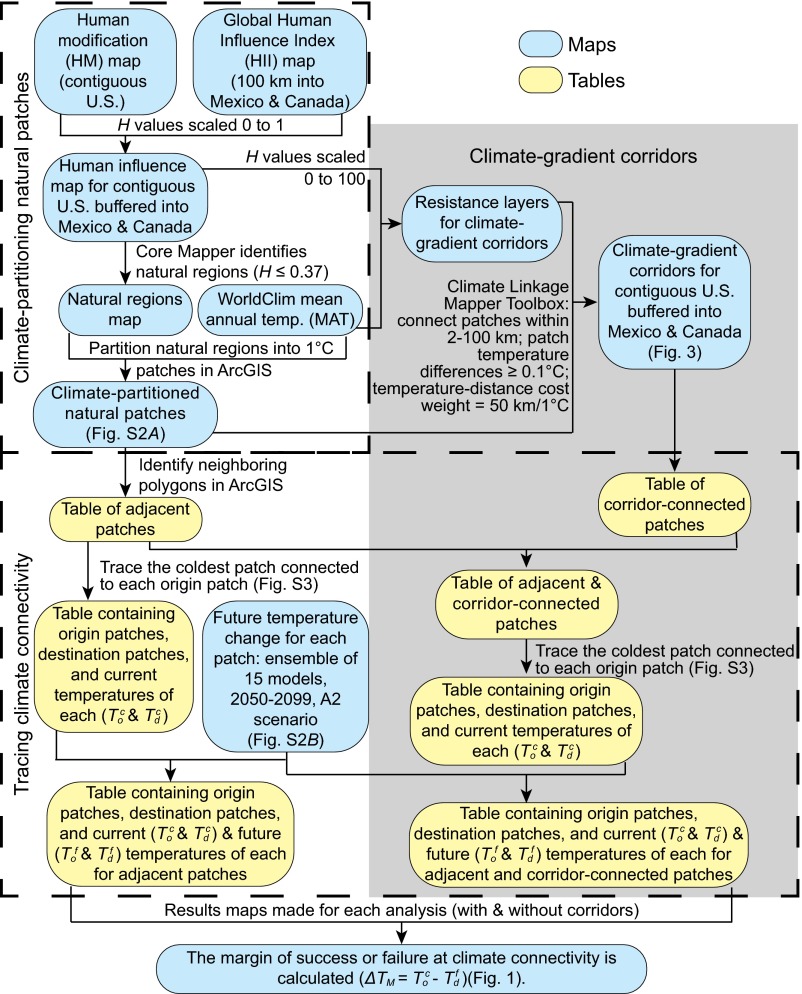
Our first step in evaluating climate connectivity was to identify the most natural tracts of land remaining within the contiguous United States (a flow chart describing our approach is provided in Fig. S1). Our analysis identifies 45% of the geographic area of the contiguous United States as natural (Fig. 1 and Fig. S2). To identify these natural regions, we used published human modification data (15, 16), which quantifies how much humans have altered the landscape by integrating data about land use, land cover, and road proximity. We identified natural regions as land having human modification values (H) less than or equal to 0.37, the 90th percentile of values from currently protected lands [status levels 1 and 2 in the Protected Area Database (17)]. We partitioned these natural regions into patches characterized by 1 °C increments (Fig. S2A). Using these temperature-partitioned patches, we identified the coolest destination patch to which any origin patch is connected, following a series of hotter to cooler patches via adjacent natural patches (Fig. S3). We calculated how much cooler the destination patch was than the origin patch (Fig. S4), and whether this difference exceeded temperature changes projected for the origin patch [using the average of temperature projections from 15 general circulation models run for the A2 emissions scenario (18) for the years 2050–2099 (19); Fig. 1, Figs. S1 and S2B, and Tables S1 and S2; other emission scenario results are reported in Tables S1 and S2]. In these analyses, we used mean annual temperature (MAT; hereafter temperature) as the target climate variable.

Fig. S1.

Methods flow chart. Blue boxes are map products; yellow boxes are data tables. Dashed lines indicate major processing stages. Climate-gradient corridor creation and analyses are highlighted in gray.

Fig. 1.

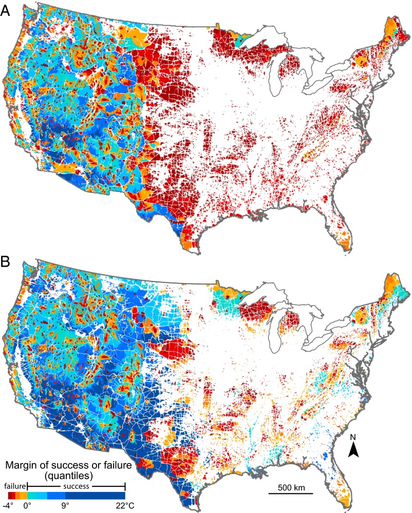
Margin of success or failure at achieving climate connectivity ($\mathrm{\Delta }{T}_M$). The margin is calculated as the current temperature of the origin ($T_o^c$) patch minus the future temperature of the destination patch ($T_d^f$) (Fig. S1). Negative temperatures, in red to orange colors, indicate a failure to achieve climate connectivity; positive temperatures, in blue colors, indicate success. (A) Without corridors. (B) With corridors.

Fig. S2.

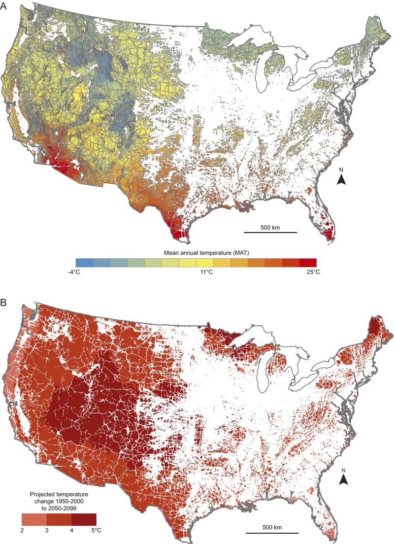
Climate maps. (A) Final climate-partitioned, natural patches. (B) One hundred-year change in patch temperature. This map displays the difference between current (1950–2000) and future (2050–2099) temperatures. Temperatures are based on the mean ensemble of 15 climate projection models (19). Future models use the A2 emissions scenario (18).

Fig. S3.

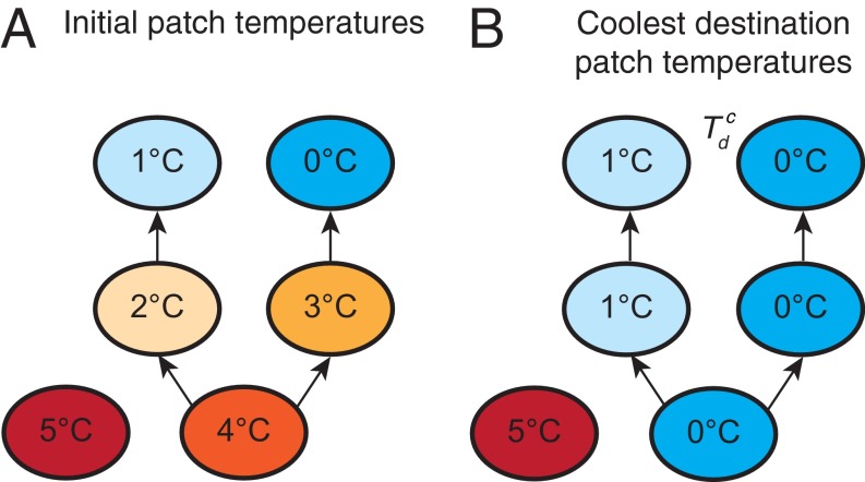
Theoretical network of patches, demonstrating the calculation of coolest destination patch temperatures ($T_d^c$). Each oval represents a patch. The colors and temperatures within each oval represent the initial temperature (A) or the destination temperature (B). Movement is in the direction of the arrows, from hotter to cooler patches. (A) Program examines each patch in turn, going from the coolest patch to the hottest patch. (B) It determines whether that patch connects to a cooler patch, selects the coolest connected patch if it connects to multiple patches, and assigns the patch a destination temperature. Unconnected patches, such as the 5 °C patch, retain their initial temperatures, as shown in A and B.

Fig. S4.

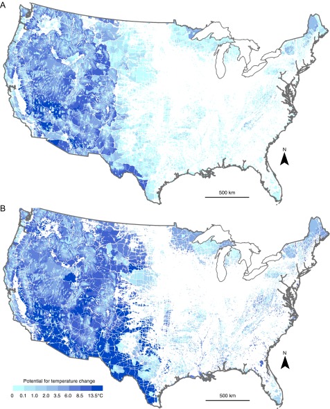
Potential for temperature change ($\mathrm{\Delta }{T}_P$). The difference between the future temperature ($T_o^f$) of each patch and the destination temperature ($T_d^f$) of that patch based on connectivity, given hotter to cooler adjacent patches (A) and corridor-connected and adjacent patches (B).

Table S1.

Percent climate connectivity success by natural area, given various climate scenarios

US patches	Adj A2, %	Adj 2.6, %	Adj 4.5, %	Adj 6.0, %	Adj 8.5, %	Cor A2, %	Cor 2.6, %	Cor 4.5, %	Cor 6.0, %	Cor 8.5, %
West	51	62	51	51	39	75	81	75	74	63
East	2	5	1	<1	0	27	43	25	21	12
Total	41	50	40	40	31	65	73	64	63	52

The margin is calculated as the current temperature of the origin patch ($T_o^c$) minus the future temperature of the destination patch ($T_d^f$) (Fig. S1). This table describes the percent area of all patches with positive margins, meaning they are successful at achieving climate connectivity. Adj indicates results for climate connectivity due to adjacency only. Cor indicates results for climate connectivity due to adjacency and corridors. The A2 emission scenario (bold) (18) is the mean ensemble of 15 projected temperature models for 2050–2099 (19). All others are RCP scenarios (RCP2.6, RCP4.5, RCP6.0, and RCP8.5) and are based upon a Model for Interdisciplinary Research on Climate 5 (MIROC5) model for each scenario (40).

Table S2.

Median (first and third quartile) margin of success or failure at climate connectivity with and without corridors given various climate scenarios

US patches	Adj A2	Adj 2.6	Adj 4.5	Adj 6.0	Adj 8.5	Cor A2	Cor 2.6	Cor 4.5	Cor 6.0	Cor 8.5
West	−1.7 °C (−3.6, 2.7)	−0.3 °C (−2.1, 4.1)	−1.5 °C (−3.4, 2.8)	−1.6 °C (−3.4, 2.7)	−3.1 °C (−5.1, 1.1)	3 °C (−2.2, 7.1)	4.3 °C (−0.9, 8.4)	3 °C (−2.1, 7.1)	2.8 °C (−2.2, 7)	1.2 °C (−3.7, 5.4)
East	−3.7 °C (−3.9, −3.3)	−2.2 °C (−2.6, −1.9)	−3.5 °C (−3.9, −3.1)	−3.8 °C (−4.2, −3.4)	−5.7 °C (−6.4, −5)	−2 °C (−3.2, −0.2)	−0.6 °C (−1.8, 1.1)	−1.9 °C (−3, −0.1)	−2.2 °C (−3.4, −0.5)	−4.1 °C (−5.3, −2.4)
Total	−3.4 °C (−3.8, −0.9)	−2 °C (−2.4, 0.5)	−3.1 °C (−3.7, −0.7)	−3.3 °C (−4, −0.8)	−5 °C (−5.9, −2.4)	−0.7 °C (−2.9, 4.4)	0.7 °C (−1.5, 5.7)	−0.6 °C (−2.8, 4.5)	−0.8 °C (−3, 4.3)	−2.7 °C (−4.8, 2.7)

The margin is calculated as the current temperature of the origin patch ($T_o^c$) minus the future temperature of the destination patch ($T_d^f$) (Fig. S1). Negative temperatures indicate a failure to achieve climate connectivity; positive temperatures indicate success. Adj indicates results for climate connectivity due to adjacency only. Cor indicates results for climate connectivity due to adjacency and corridors. The A2 emission scenario (bold) (18) is the mean ensemble of 15 projected temperature models for 2050–2099 (19). All others are RCP scenarios (RCP2.6, RCP4.5, RCP6.0, and RCP8.5) and are based upon a MIROC5 model for each scenario (40).

Results and Discussion

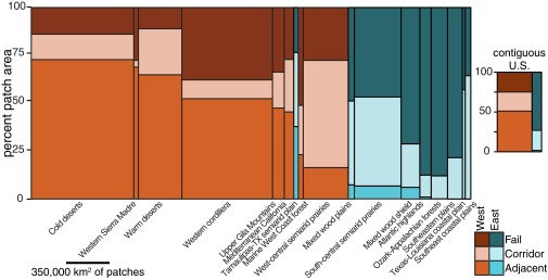
Only 41% of natural land area achieves climate connectivity if movement is assumed only to occur between a series of adjacent natural patches (Fig. 1A and Table S1). The western United States has higher climate connectivity (51% of natural land area) compared with the eastern United States (2% of natural land area) (Fig. 2 and Table S1; the east-west division is illustrated in Fig. S5). Once we established this baseline, we asked to what degree increasing connectivity by adding corridors between natural patches increases climate connectivity and where establishing corridors would be most effective.

Fig. 2.

Percentage of natural area per ecoregion that succeeds at achieving climate connectivity. Orange colors are western ecoregions; teal colors are eastern ecoregions. Bright colors are climate connectivity success, given adjacency only; pale colors are the additional success given corridors; and dark colors are failures. Bar width indicates the natural area per ecoregion, and bars are sorted by decreasing success, given adjacency only. Three missing ecoregions contained too little natural area to display: Everglades (0% adjacent success, 0% corridor success), central plains (0% adjacent success, 1.6% corridor success), and temperate prairies (0.1% adjacent success, 10% corridor success). (Inset) Overall success rates in the West vs. East. Ecoregion locations and the east–west division are provided in Fig. S5.

Fig. S5.

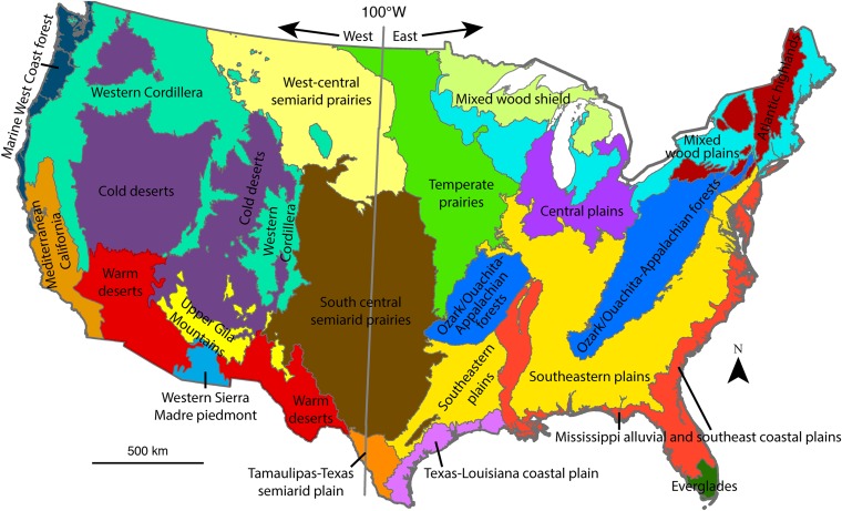
Geographic and ecological divisions. We used the 100°W longitudinal line to divide the arid West from the moister, eastern United States. Colored divisions represent the 20 level II Environmental Protection Agency ecological regions used for analyses (47).

Climate-gradient corridors identify movement routes between patches that follow monotonically decreasing temperature gradients while simultaneously minimizing cumulative resistance to movement (20). Resistance increases with degree of human impact (movement cost) and climate gradient steepness or reversal (Methods and Eq. 1). Urban centers impose high traversal costs, whereas minimally disturbed areas are more conducive to traversal. Using this method, we created climate-gradient corridors for the contiguous United States (Fig. 3, SI Methods, and Figs. S1 and S6).

Fig. 3.

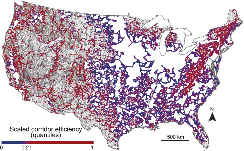
Corridor efficiency scaled to the maximum value. Patches are gray, and corridors are blue to red from highest to lowest relative efficiency. Corridor efficiency measures how challenging it is to traverse the corridor due to human impacts and the thermal gradient per kilometer of corridor. More efficient corridors are less challenging to traverse and may be less expensive to conserve and restore because they generally have lower human impacts.

Fig. S6.

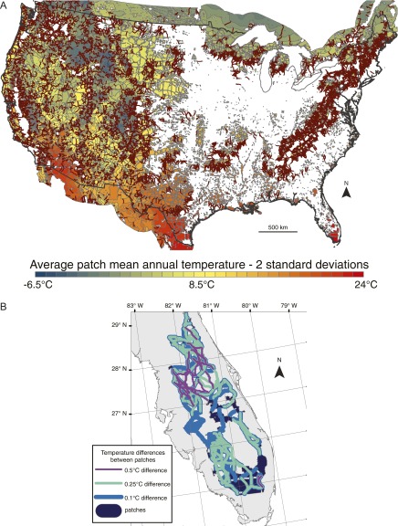
Climate-gradient corridor sensitivity tests. (A) Climate-gradient corridor map that demonstrates the need to revise the default method (20) for designating temperature differences between patches. The map requires a 1 °C difference in minimum patch temperatures. Dark-red lines are least-cost climate gradient corridors. Note that many patches, particularly in Florida, Texas, and the Midwest, are isolated, without corridor connections or adjacent patches. (B) Florida sensitivity map of temperature differences between patches.

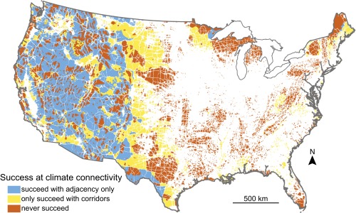
Introducing corridors between patches separated by up to 100 km of human-impacted (H > 0.37) land increases nationwide climate connectivity to 65% of natural land area and allows species living in natural patches to adjust to a median of 2.7 °C more temperature change (Fig. 1B and Tables S1 and S2). If we limit maximum corridor length to 10 km, we still achieve climate connectivity for 60% of natural land area. Adding corridors increases climate connectivity in the western and eastern United States by similar percentage points of natural land area (24% and 25%, respectively), resulting in more success in the West (75%) than the East (27%) (Fig. 2, Figs. S5 and S7, and Table S1).

Fig. S7.

Improvements due to corridors. Patches that never achieve success (orange), succeed with adjacency only (without the additional facilitation of corridors, blue), and succeed only if corridors are present (yellow) are shown.

We would not have expected proportional improvement in climate connectivity to be similar in the eastern and western United States (Figs. 1 and 2), given that temperatures are projected to increase more in the West (Fig. S2B). However, the West also contains colder mountain ranges and steeper climate gradients (Fig. S2A). Cold regions provide target destinations for tracking changing climate, allowing species living in temperate areas that are projected to warm to achieve climate parity even after the entire landscape warms. The lack of natural lands and the basin of higher temperatures in the Midwest (Fig. S2A) prevent movement between the East and West or into the north-central regions, where cool, natural land patches persist.

When assessing climate connectivity by ecoregion, we find that connecting low-elevation regions, notably the semiarid prairies and coastal plains, provides the greatest improvement from corridors (Figs. 1 and 2; ecoregion names and locations are provided in Fig. S5). The west and south-central semiarid prairies experience large increases in climate connectivity (56 and 47 percentage point increased climate connectivity area) when fragmented natural regions are connected to the cool Western Cordillera region (Figs. 1 and 2). The Texas-Louisiana coastal plains and Mississippi alluvial and southeast coastal plains experience improvements (64 and 57 percentage point increased climate connectivity area) through connections into the Ozark, Ouachita, and Appalachian mountain systems (Figs. 1 and 2). The smallest improvements from corridors are seen in two types of areas: (i) ecoregions distant from cool montane regions, such as the Everglades, the central plains, or the temperate prairies (0, 2, and 10 percentage point increased climate connectivity area) or (ii) certain montane regions, including the Western Cordillera and Western Sierra Madre (4 and 10 percentage point increased climate connectivity area), where natural regions are already adjacent and mountaintops create climate islands (Figs. 1 and 2 and Fig. S7).

To evaluate the differences in benefits among corridor placements further, we explored where corridors would be least challenging to construct. We examined cumulative resistance and corridor efficiency. We define cumulative resistance as the summed total of all cost-weighted distances of the corridors necessary to reach the cool destination patch and corridor efficiency as the cumulative resistance per kilometer of corridor. Corridor efficiency thus represents a combination of human impact and temperature gradients. More efficient corridors are less challenging to traverse and may be less expensive to purchase, conserve, and restore, because they generally have lower human impacts. Here, we assess only those patches that could achieve climate connectivity because of corridors.

Average cumulative resistance of eastern climate corridors is 4.3-fold higher than western corridors (Welch’s t = 28.8, df = 1455, P < 0.0001). However, corridor efficiency in the East is 0.89-fold corridor efficiency in the West (Welch’s t = −18.4, df = 2622, P < 0.0001; Fig. 3). Thus, eastern corridors cross less intensely human-impacted land and/or shallower climate gradients but across longer corridor distances (Fig. 3). This finding is further demonstrated by restricting corridor length to 10 km, where eastern climate connectivity success drops from 27 to 16%.

Similarly, ecoregions with the highest cumulative resistance are also most benefited by corridors. Three southeastern ecoregions, the Mississippi alluvial and southeast coastal plains, Texas-Louisiana coastal plain, and west and south central semiarid prairies, contribute 65% of total cumulative resistance across all 20 ecoregions (Fig. 2 and Fig. S5) but also have the best corridor efficiency (Fig. 3).

Eastern corridors, particularly in those three southeastern ecoregions, have a larger proportional impact and demonstrate better corridor efficiency (Fig. 3). Climate connectivity increases by 13-fold in the East (from 2 to 27%), and this increase may be more critical for overall dispersal than the 0.5-fold increase in the West (51–75%) (Figs. 1 and 2, Fig. S7, and Table S1). Moreover, based on projected species range shifts, many more individual vertebrate species will likely need to track suitable climates through the southeastern United States and Appalachian Mountains than through the western mountain systems (21). In particular, the regions that have both the highest improvement with corridors and a high volume of vertebrates needing to traverse that landscape (21) are the coastal plains of Texas, Louisiana, Mississippi, and the southeastern United States (Figs. 1–3 and Fig. S5).

Under projected climate scenarios, corridors will be a critical strategy for allowing species to respond to warmer temperatures (Fig. S7). The A2 emissions scenario used here is moderate, comparable to representative concentration pathway 4.5 (RCP4.5) (Tables S1 and S2). If climate change is more severe, even corridor-assisted connectivity may be insufficient, because hotter temperatures produce fewer, smaller cool destinations for species (Tables S1 and S2). Additionally, the natural land patches we identified provide large tracts of land and many small, intermediate patches to serve as steppingstones (Fig. S2A). However, as human impacts increase, these steppingstones may disappear (22–24).

Climate connectivity does not guarantee species persistence in the face of climate change. High connectivity only provides the potential for species to disperse to temperatures similar to those temperatures they experience today. Destination patches may be too small to allow sufficient population sizes for survival (25–27). Also, temperatures are changing so rapidly that even species with the potential to disperse may still not disperse quickly enough to reach future areas of climate suitability (28–30).

However, even without increasing connectivity, our findings do not necessarily portend wide-scale extinctions. Many species have relatively broad temperature tolerances and may survive even hotter conditions than they occupy today. Species may also evolve or undergo phenotypically plastic shifts to enable further survival. Our analyses likely underestimate the ability of many climate-limited species to persist in cooler microhabitats (31–33), which our 1-km² spatial resolution with 10-km² minimum patch sizes may be too coarse to identify. This issue of spatial resolution is especially relevant in montane regions, where climate variation is high, and small regions with different temperatures were necessarily lumped to create 10-km² patches. The use of MAT as our climate variable of interest may also obscure important climate-driven impacts for certain habitats or certain types of species. For example, in California, the strong seasonal fluctuations characteristic of this region’s Mediterranean climate mean that the use of the MAT climate variable could obscure the more relevant changes in seasonal climatic variation in this region (34). Analyses that focus on species movement needs with respect to small-scale variation and diverse climate variables could lead to more optimistic results.

Under rapidly changing climatic conditions, in which many species must adapt or move to preclude extinction, fragmentation limits one critical coping strategy. Of course, human-impacted land does not hinder all organisms. Some birds or wind-dispersed seeds and insects may be able to traverse hundreds of kilometers of inhospitable lands, but even these species’ movements are made easier by the introduction of corridors (35–37). Those species that struggle with dispersal across roads, through cities, and across agricultural fields (e.g., many amphibians, reptiles, plants, small mammals) need an alternate solution. Knowing where to focus conservation efforts is crucial for these species and for the future of biodiversity. We find that corridors will be critical for movement, given high habitat fragmentation levels. This need is particularly critical in the southeastern United States and regions with fragmented landscapes and few nearby climatic refuges. Facilitating movement between natural lands will greatly improve the chances of species being able to track suitable climates.

SI Methods

Climate Linkage Mapper Toolbox requires that several parameters are set: distances between patches, temperature differences between patches, and temperature-distance weight. For two patches to be connected, we required the destination patch to be within 2–100 km. The low value, 2 km, is the shortest possible distance between two patches, given that we are working at a 1-km resolution. The high value, 100 km, represents a long, but reasonable, planning unit. We also calculated success rates using shorter, 10-km corridors because these lengths may be more realistic for some planning purposes.

We required that the average temperature of the pixels within a destination patch must be cooler than the pixels of the origin patch by 0.1 °C. This choice differs from the choice of Nuñez et al. (20), who required the minimum temperature (mean temperature − 2 SD) between patches to differ by at least 1 °C. Our approach was better suited to our climate-partitioned patches because we did not need to compensate for large temperature variation within patches. Moreover, requiring 1 °C temperature differences meant that thousands of patches would have been left unconnected (Fig. S6A). Thus, we compared the average temperatures within our climate-partitioned patches. We examined climate corridors in peninsular Florida to determine the minimum climate difference necessary to increase connectivity (Fig. S6B). Our goal was to maximize connectivity across the contiguous United States, therefore maximizing the opportunities for achieving climate connectivity. We lowered the threshold to 0.1 °C to allow as many patches as possible to be included in our ultimate network.

We selected the same temperature-distance weight of 50 km per 1 °C as Nuñez et al. (20). This weight penalizes temperature changes relative to the cost value for distance traveled, so that corridors avoid excessive temperature changes between origin and destination patches.

Methods

Our study area includes the contiguous United States buffered by 100 km into Mexico and Canada. We performed all statistical analyses on the contiguous United States only. We analyzed maps at 1-km resolution, projected into North American Datum (NAD) 1983 Albers equal area conic projections. An outline of all methods can be seen in Fig. S1.

Identifying and Climate-Partitioning Natural Patches.

To identify natural regions, we used a map that depicts human impacts by quantifying the degree of human modification (H) with values ranging from 0–1.0 (low to high) (15). This map combines nearly a dozen layers of anthropogenic stressors with empirical validation to create a layer for the contiguous United States that integrates data about land use, land cover, and road proximity (15). It has been thoroughly vetted to establish consistent values nationwide, but does not extend beyond the borders of the contiguous United States [details are provided by Theobald (15)]. Not wanting to truncate climate gradients artificially at political borders, we used a 100-km buffer extending into Canada and Mexico using the Human Influence Index (HII) map (16). The HII map does not integrate the full set of land-use data used by the human modification map, but nonetheless provides informative H values within the buffer regions.

We identified a threshold for the H value that represents relatively natural land, given the level of human impact across the contiguous United States. Following protocols established by the Western Governors’ Association, we extracted all H values located within the most protected lands nationwide [Gap Analysis Program (GAP) status level 1 and 2 lands in the Protected Areas Database (17)]. These extracted H values represent the human impact levels within the most protected portions of the contiguous United States. However, not all land within protected areas is perfectly natural. Some portion represents roads, visitor’s centers, and other human modifications that allow for the enjoyment or exploitation of protected areas. We examined the histogram of H values found within the GAP status 1 and 2 lands and also mapped varying percentiles (75th–95th) of those H values. We determined that the 90th percentile of H values within GAP status 1 and 2 lands (H = 0.37) identifies natural lands within protected areas minus natural lands in highly modified areas. We used this value to identify natural regions throughout the study area using the Core Mapper tool within the Gnarly Landscape Utilities package (38). This tool passed a 10-km² (1.784-km radius) moving window over the map to identify high-integrity natural regions greater than 10 km² and with average H values ≤0.37.

Once we identified natural portions of the contiguous United States, we then developed a method to partition those natural regions by temperature. This step served two purposes. First, it created discrete land patches that have endemic climate characteristics, which we used to establish climate gradients. Second, by partitioning natural areas, we reduced the amount of within-patch climate variation. Within-patch climate variation can obscure climate differentials between patches, and therefore obscure the connections necessary to follow those climate gradients.

To partition the natural regions, we used a 30-arc-second MAT (hereafter called temperature) climate layer from the WorldClim global climate layers (∼1950–2000), resampled to 1-km² resolution (39). We converted the natural regions to a raster format and extracted the temperature value for each pixel. To create climate partitions within the large natural regions, we then smoothed the temperature values across the layer using a Gaussian moving window (radius = 15 km, SD = 5), reclassified the values to 1 °C increments, aggregated patches in the same temperature increment that were within 2 km of one another, and deleted any patches smaller than 10 km². This process resulted in 11,256 individual patches partitioned by 1 °C and aggregated across roads and other small regions of human impact (Fig. S2A). Climate-partitioned natural regions are hereafter referred to as patches. The 1-km² resolution temperature within each patch was then used for all subsequent analyses.

Future Temperature Projections.

To evaluate climate connectivity, we report results for the mean ensemble of 15 models for a future (2050–2099) time period [A2 emission scenario (18): continually increasing rate of greenhouse gas emissions] (19). We use mean current MAT (1950–2000) and mean future MAT (2050–2099) for all primary calculations. Those layers were then subtracted to create a map of projected temperature change (Fig. S2B) that was used in conjunction with the current WorldClim layer. This same process was completed for Model for Interdisciplinary Research on Climate 5 (MIROC5) models of four RCP scenarios: RCP2.6, RCP4.5, RCP6.0, and RCP8.5 (40).

Tracing Climate Connectivity, Given Adjacent Patches.

Once the patches were identified and current and future patch temperatures were compiled, we sought to determine the coldest temperature that a population living in each patch could potentially reach were it to traverse natural areas, moving from hotter to cooler adjacent patches. In ArcGIS 10.2 (41), we first created a table representing all pairs of adjacent patches using the native “Polygon Neighbors” toolbox. We then used R (42) to order these adjacent patch tables so that the hotter patch within each adjacent pair was an origin patch and the cooler patch was the destination.

Using this network of hotter to cooler adjacent patches, we wrote a script in R (42) that allows cool temperatures to propagate backward through the network (i.e., from cooler destination patches to hotter origin patches) and finally provides the coolest current destination temperature ($T_d^c$; hereafter destination temperatures) to which each patch is connected. For example, if we examine the network in Fig. S3A, population movement would be expected to go from hotter to cooler patches, as indicated by the arrows. In our script, we would ask whether the coolest patch, which is 0 °C, connects to any cooler patches. In this case, and for the next hotter patch (1 °C), the answer would be “no.” The 2 °C patch connects to the 1 °C patch. It would therefore assume a destination temperature of 1 °C, as seen in Fig. S3B. Similarly, the 3 °C patch would assume a destination temperature of 0 °C. Next, the 4 °C patch in Fig. S3A connects to two patches, which have new destination temperatures of 1 °C and 0 °C (those patches whose initial temperatures were 2 °C and 3 °C), respectively. The 4 °C patch assumes the destination temperature of the cooler of those two patches, which is 0 °C (Fig. S3). Any patch that has no adjacency, such as the 5 °C patch, keeps its initial temperature as its destination temperature.

Next, we wanted to determine which patches achieve climate connectivity. Climate connectivity is achieved when patches are connected to cool regions sufficiently such that the future temperature of the destination patch ($T_d^f$) is the same as or cooler than the current temperature of the origin patch ($T_o^c$; Fig. S1). By subtracting these variables, we determine the margin of success or failure at climate connectivity ($\mathrm{\Delta }{T}_M$; Fig. 1A and Fig. S1). If the margin of success or failure is positive, climate connectivity is achieved, meaning that organisms living in that patch could track their current temperatures through adjacent patches, given projected climate change. Table S1 depicts the percentage of climate connectivity success by natural land area for the five future emission scenarios assessed. Table S2 depicts the median and first and third quartiles of the margin of success or failure ($\mathrm{\Delta }{T}_M$) for each of these scenarios. The range of emission scenarios gives us a sense of what could happen, given best- or worst-case scenarios regarding rising temperatures.

Creating a Network of Climate-Gradient Corridors.

Once we had determined climate connectivity based upon adjacent patches, we wanted to know how and where climate connectivity would be improved if we implemented corridors. To answer this question, we created a network of climate-gradient corridors for the contiguous United States using the Climate Linkage Mapper Toolbox (43). This toolbox implements the climate-gradient corridor method introduced by Nuñez et al. (20), which identifies movement routes between patches that follow monotonic climate (i.e., temperature) gradients while simultaneously minimizing cumulative resistance to movement created by human modifications. The toolbox creates a network of least-cost corridors that link neighboring patches to each other. To calculate least-cost corridors, the climate-gradient corridor method modifies the standard cost-distance corridor model by using an anisotropic equation that not only penalizes for traversing additional distance but also adds cost both for moving through human-dominated lands and for temperature changes (20). Penalizing for temperature changes enables the software to prioritize paths that traverse monotonic climate gradients, avoiding movement through particularly hot or cool areas. This equation calculates a map of distance costs (D_c) for moving from a focal cell to one of the eight neighboring cells and repeats until reaching the destination patch:

$$D_c=\left[\left({\mathit{C}}_o+C_n\right)/2\right]D_e+\left|T_o-T_n\right|W,$$ [1]

where C_o is the cost of the origin cell, C_n is the cost of the least-cost neighboring cell, D_e is the Euclidean distance between the cells, and the temperature-distance weight, W, is 50 km per 1 °C. The D_c values of the cells that fall along the least-cost path are then summed, creating the cost-weighted distance of the corridor.

We used our climate-partitioned patch layer as the “core area” layer for the toolbox. Our human modification layer buffered by the HII maps served as the resistance layer, whose values provided movement costs. We normalized the H values from 1 to 100, with low values indicating the least impacted regions. We used the WorldClim global climate layer (∼1950–2000), resampled to 1-km² resolution (39) for each cell’s MAT value. We used GRASS v7.0, ArcGIS 10.2, and Climate Linkage Mapper Toolbox v10.8 (41, 43, 44).

The Climate Linkage Mapper Toolbox requires several a priori parameter designations: minimum and maximum distance between patches (2 km and 100 km), maximum temperature difference required between patches (0.1 °C), and the relative cost penalty for temperature and distance (50 km per 1 °C). Using these parameters, the Climate Linkage Mapper Toolbox created the final corridors used in our analyses (Fig. 3). Sensitivity analyses used to guide our parameterization are provided in SI Methods and Fig. S6.

Tracing Climate Connectivity, Given Corridors and Adjacent Patches.

In creating these corridors, the Climate Linkage Mapper Toolbox also created a corridor connectivity table with hotter origin patches and cooler destination patches that could be reached by moving up to 100 km across human-impacted (H ≥ 0.37) regions. We merged this corridor connectivity table with our initial adjacency table (created above) to create a full network of patches that could be traversed by traveling through corridors or through cooler adjacent patches. We used this network to determine how much facilitating movement through human-dominated regions could improve climate connectivity.

Using this connectivity network that integrated patch adjacency and corridor connectivity, we used the same program as described above to trace the destination temperature, given the patch connectivity ($T_d^c$; Fig. S3). In addition, we calculated cumulative resistance for each patch by summing the costs of the corridors used to achieve each patch’s destination. No cost was assigned for using adjacent patches.

To determine which patches achieve climate connectivity given patch adjacency and corridor connectivity, we used these newly calculated destination temperatures ($T_d^f$) to calculate the margin of success or failure at climate connectivity ($\mathrm{\Delta }{T}_M$; Fig. 1B and Fig. S1). If the margin of success or failure is positive, climate connectivity is achieved, meaning that organisms living in that patch could track their current temperatures through a combination of adjacent patches and corridors, given projected climate change.

We again calculated success rates and median and first and third quartile temperature margins ($\mathrm{\Delta }{T}_M$) that would occur under five emission scenarios (Tables S1 and S2). Additionally, we calculated success rates for a scenario in which corridors are ≤10 km in length for the A2 emission scenario. Including only these shorter corridors decreased the percentage points of natural land area that succeeds at achieving climate connectivity by 4% in the West, 11% in the East, and 5% overall.

Geographic Analyses of Climate Connectivity.

Our final map identifies the patches that failed to achieve climate connectivity, given adjacency alone, but then succeeded once corridors were introduced (Fig. S7).

We compared the number of patches, the potential for temperature change achievable, and the margins of success or failure in the eastern vs. western United States (Fig. 2 and Tables S1 and S2). We performed t tests to estimate where differences were significant. For these analyses, the contiguous United States was divided at 100°W longitude, which has long been held as a general dividing line between the more arid, western United States and the moister East and the resultant disparities in human settlement patterns (45, 46) (Fig. S5). We additionally compared the temperature changes achievable and the margins of success or failure within level II Environmental Protection Agency ecological regions (47) (Fig. 2 and Fig. S5).

References

- 1.IPCC 2013. Summary for Policymakers. Climate Change 2013: The Physical Science Basis. Contribution of Working Group I to the Fifth Assessment Report of the Intergovernmental Panel on Climate Change, eds Stocker TF, et al. (Cambridge University Press, New York)
- 2.Moritz C, et al. Impact of a century of climate change on small-mammal communities in Yosemite National Park, USA. Science. 2008;322(5899):261–264. doi: 10.1126/science.1163428. [DOI] [PubMed] [Google Scholar]
- 3.Parmesan C. Ecological and evolutionary responses to recent climate change. Annu Rev Ecol Evol Syst. 2006;37(1):637–669. [Google Scholar]
- 4.Chen I-C, Hill JK, Ohlemüller R, Roy DB, Thomas CD. Rapid range shifts of species associated with high levels of climate warming. Science. 2011;333(6045):1024–1026. doi: 10.1126/science.1206432. [DOI] [PubMed] [Google Scholar]
- 5.Holderegger R, Di Giulio M. The genetic effects of roads: A review of empirical evidence. Basic Appl Ecol. 2010;11(6):522–531. [Google Scholar]
- 6.Corlett RT, Westcott DA. Will plant movements keep up with climate change? Trends Ecol Evol. 2013;28(8):482–488. doi: 10.1016/j.tree.2013.04.003. [DOI] [PubMed] [Google Scholar]
- 7.Trombulak SC, Frissell CA. Review of ecological effects of roads on terrestrial and aquatic communities. Conserv Biol. 2000;14(1):18–30. [Google Scholar]
- 8.Sinervo B, et al. Erosion of lizard diversity by climate change and altered thermal niches. Science. 2010;328(5980):894–899. doi: 10.1126/science.1184695. [DOI] [PubMed] [Google Scholar]
- 9.Kerr JT, et al. Climate change impacts on bumblebees converge across continents. Science. 2015;349(6244):177–180. doi: 10.1126/science.aaa7031. [DOI] [PubMed] [Google Scholar]
- 10.Heller NE, Zavaleta ES. Biodiversity management in the face of climate change: A review of 22 years of recommendations. Biol Conserv. 2009;142(1):14–32. [Google Scholar]
- 11.Kostyack J, Lawler JJ, Goble DD, Olden JD, Scott JM. Beyond reserves and corridors: Policy solutions to facilitate the movement of plants and animals in a changing climate. Bioscience. 2011;61(9):713–719. [Google Scholar]
- 12.Tewksbury JJ, et al. Corridors affect plants, animals, and their interactions in fragmented landscapes. Proc Natl Acad Sci USA. 2002;99(20):12923–12926. doi: 10.1073/pnas.202242699. [DOI] [PMC free article] [PubMed] [Google Scholar]
- 13.Beier P, Brost B. Use of land facets to plan for climate change: Conserving the arenas, not the actors. Conserv Biol. 2010;24(3):701–710. doi: 10.1111/j.1523-1739.2009.01422.x. [DOI] [PubMed] [Google Scholar]
- 14.Gilbert-Norton L, Wilson R, Stevens JR, Beard KH. A meta-analytic review of corridor effectiveness. Conserv Biol. 2010;24(3):660–668. doi: 10.1111/j.1523-1739.2010.01450.x. [DOI] [PubMed] [Google Scholar]
- 15.Theobald DM. A general model to quantify ecological integrity for landscape assessments and US application. Landsc Ecol. 2013;28(10):1859–1874. [Google Scholar]
- 16.Wildlife Conservation Society (WCS), Center for International Earth Science Information Network (CIESIN) 2005. Last of the Wild Project, Version 2, 2005 (LWP-2): Global Human Influence Index (HII) Dataset (Geographic). Available at sedac.ciesin.columbia.edu/data/set/wildareas-v2-human-influence-index-geographic. Accessed June 12, 2012.
- 17.US Geological Survey National Gap Analysis Program 2012. Protected Areas Database of the United States. Available at gapanalysis.usgs.gov/padus/. Accessed October 1, 2012.
- 18.Nakicenovic N, et al. 2000. Special Report on Emissions Scenarios, eds Nakicenovic N, Swart R (Cambridge Univ Press, Cambridge, UK)
- 19.Girvetz EH, et al. Applied climate-change analysis: The climate wizard tool. PLoS One. 2009;4(12):e8320. doi: 10.1371/journal.pone.0008320. [DOI] [PMC free article] [PubMed] [Google Scholar]
- 20.Nuñez TA, et al. Connectivity planning to address climate change. Conserv Biol. 2013;27(2):407–416. doi: 10.1111/cobi.12014. [DOI] [PubMed] [Google Scholar]
- 21.Lawler JJ, Ruesch AS, Olden JD, McRae BH. Projected climate-driven faunal movement routes. Ecol Lett. 2013;16(8):1014–1022. doi: 10.1111/ele.12132. [DOI] [PubMed] [Google Scholar]
- 22.Jantz CA, Goetz SJ, Donato D, Claggett P. Designing and implementing a regional urban modeling system using the SLEUTH cellular urban model. Comput Environ Urban Syst. 2010;34(1):1–16. [Google Scholar]
- 23.Foley JA, et al. Global consequences of land use. Science. 2005;309(5734):570–574. doi: 10.1126/science.1111772. [DOI] [PubMed] [Google Scholar]
- 24.Defries RS, Bounoua L, Collatz GJ. Human modification of the landscape and surface climate in the next fifty years. Glob Change Biol. 2002;8(5):438–458. [Google Scholar]
- 25.Niebuhr BBS, et al. Survival in patchy landscapes: The interplay between dispersal, habitat loss and fragmentation. Sci Rep. 2015;5:11898. doi: 10.1038/srep11898. [DOI] [PMC free article] [PubMed] [Google Scholar]
- 26.Haddad NM, et al. Habitat fragmentation and its lasting impact on Earth’s ecosystems. Sci Adv. 2015;1(2):e1500052. doi: 10.1126/sciadv.1500052. [DOI] [PMC free article] [PubMed] [Google Scholar]
- 27.Elsen PR, Tingley MW. Global mountain topography and the fate of montane species under climate change. Nat Clim Chang. 2015;5(8):772–776. [Google Scholar]
- 28.Schloss CA, Nuñez TA, Lawler JJ. Dispersal will limit ability of mammals to track climate change in the Western Hemisphere. Proc Natl Acad Sci USA. 2012;109(22):8606–8611. doi: 10.1073/pnas.1116791109. [DOI] [PMC free article] [PubMed] [Google Scholar]
- 29.Loarie SR, et al. The velocity of climate change. Nature. 2009;462(7276):1052–1055. doi: 10.1038/nature08649. [DOI] [PubMed] [Google Scholar]
- 30.Dobrowski SZ, et al. The climate velocity of the contiguous United States during the 20th century. Glob Change Biol. 2013;19(1):241–251. doi: 10.1111/gcb.12026. [DOI] [PubMed] [Google Scholar]
- 31.Rull V. Microrefugia. J Biogeogr. 2009;36(3):481–484. [Google Scholar]
- 32.Dobrowski SZ. A climatic basis for microrefugia: The influence of terrain on climate. Glob Change Biol. 2011;17(2):1022–1035. [Google Scholar]
- 33.Hannah DM, Malcolm IA, Soulsby C, Youngson AF. A comparison of forest and moorland stream microclimate, heat exchanges and thermal dynamics. Hydrol Processes. 2008;22(7):919–940. [Google Scholar]
- 34.Ackerly DD, Cornwell WK, Weiss SB, Flint LE, Flint AL. A Geographic Mosaic of Climate Change Impacts on Terrestrial Vegetation: Which Areas Are Most at Risk? PLoS One. 2015;10(6):e0130629. doi: 10.1371/journal.pone.0130629. [DOI] [PMC free article] [PubMed] [Google Scholar]
- 35.Alsos IG, et al. Frequent long-distance plant colonization in the changing Arctic. Science. 2007;316(5831):1606–1609. doi: 10.1126/science.1139178. [DOI] [PubMed] [Google Scholar]
- 36.Herrmann JD, et al. Connectivity from a different perspective: comparing seed dispersal kernels in connected vs. unfragmented landscapes. Ecology. 2016;97(5):1274–1282. doi: 10.1890/15-0734.1. [DOI] [PubMed] [Google Scholar]
- 37.Damschen EI, et al. The movement ecology and dynamics of plant communities in fragmented landscapes. Proc Natl Acad Sci USA. 2008;105(49):19078–19083. doi: 10.1073/pnas.0802037105. [DOI] [PMC free article] [PubMed] [Google Scholar]
- 38.Shirk AJ, McRae BH. 2013. Gnarly Landscape Utilities: Core Mapper User Guide (The Nature Conservancy, Fort Collins, CO). Available at www.circuitscape.org/gnarly-landscape-utilities. Accessed August 4, 2012.
- 39.Hijmans RJ, Cameron SE, Parra JL, Jones PG, Jarvis A. Very high resolution interpolated climate surfaces for global land areas. Int J Climatol. 2005;25(15):1965–1978. [Google Scholar]
- 40.Ramirez J, Jarvis A. 2008. High resolution statistically downscaled future climate surfaces (International Center for Tropical Agriculture; CGIAR Research Program on Climate Change, Agriculture and Food Security, Cali, Columbia). Available at ccafs-climate.org/data/. Accessed November 15, 2015.
- 41.ESRI 2013. ArcGIS Desktop: Release 10.2 (ESRI, Redlands, CA)
- 42.Urbanek S, Bibiko H-J, Iacus SM. 2014. R. Available at www.r-project.org. Accessed February 1, 2012.
- 43.Kavanagh DM, Nuñez TA, McRae BH. 2013. Climate Linkage Mapper Connectivity Analysis Software. Available at www.circuitscape.org/linkagemapper. Accessed October 28, 2012.
- 44.GRASS Development Team 2012. Geographic Analysis Support System (GRASS) Software. Available at grass.osgeo.org. Accessed October 28, 2012.
- 45.Powell JW. 1879. Report on the lands of the arid region of the United States with a more detailed account of the land of Utah with maps. Available at https://pubs.er.usgs.gov/publication/70039240. Accessed December 3, 2015.
- 46.Maizel M. 1998. Historical interrelationships between population settlement and farmland in the conterminous United States, 1790 to 1992 (Washington, DC). Available at landcover.usgs.gov/luhna/chap2.php. Accessed February 3, 2016.
- 47.US Environmental Protection Agency 1997. Ecoregions of North America. Available at https://www.epa.gov/wed/pages/ecoregions.htm. Accessed November 5, 2016. [PubMed]