

Abstract
Motivation: Topological domains have been proposed as the backbone of interphase chromosome structure. They are regions of high local contact frequency separated by sharp boundaries. Genes within a domain often have correlated transcription. In this paper, we present a computational efficient spectral algorithm to identify topological domains from chromosome conformation data (Hi-C data). We consider the genome as a weighted graph with vertices defined by loci on a chromosome and the edge weights given by interaction frequency between two loci. Laplacian-based graph segmentation is then applied iteratively to obtain the domains at the given compactness level. Comparison with algorithms in the literature shows the advantage of the proposed strategy.
Results: An efficient algorithm is presented to identify topological domains from the Hi-C matrix.
Availability and Implementation: The Matlab source code and illustrative examples are available at http://bionetworks.ccmb.med.umich.edu/
Contact: indikar@med.umich.edu
Supplementary information: Supplementary data are available at Bioinformatics online.
1 Introduction
Chromosome conformation capture techniques (3C, 4C, Hi-C) have yielded an unprecedented level of information about genome organization, and many studies are now exploring the relationship between genome structure and transcription (Cavalli and Misteli, 2013; Chen et al., 2015b; Gorkin et al., 2014). Chromosome conformation capture studies suggest that eukaryotic genomes are organized into structures called topological domains (or topologically associating domains, TADs). Topological domains can be defined as linear units of chromatin that fold as discrete three-dimensional (3D) structures tending to favor internal chromatin interactions (Dixon et al., 2012; Nora et al., 2012). A majority of regulatory protein binding sites localize within topological domains. This suggests that sites associated with domain borders represent a functionally different subclass of alleles that delimit regions containing housekeeping genes and insulator sites (Van Bortle et al., 2014). Detecting the topological domains is thus helpful for studying the relationship between chromosome organization and gene transcription. For additional works on delineating structural domains (see Le Dily et al., 2014; Lévy-Leduc et al., 2014; Liu et al., 2012; Pope et al., 2014; Sexton et al., 2012).
Topological domains can be detected using data from Hi-C, which allows genome-wide identification of chromatin contacts. The Hi-C method probes the 3D architecture of the whole genome by coupling proximity-based ligation with massively parallel sequencing. The Hi-C data matrix records the contact frequency between pairs of loci. Topological domains, as regions that have high intra-contacts, are characterized by diagonal blocks in the Hi-C matrix. To identify topological domains, in (Dixon et al., 2012) the authors employed a Hidden Markov Model (HMM) on the directionally index from a Hi-C matrix to determine regions initiated by significant downstream chromatin interactions and terminated by a sequence of significant upstream interactions. Filippova et al. (2014) formulated the identification problem by maximizing the domain total reads and introduced a dynamic programming algorithm to solve the problem with a given scale parameter.
These methods perform analysis on a 1D read index or on a 2D image segmentation subblock, and they suffer from sensitivity to initialization (e.g. HMM model parameter adjustment), and high computational complexity (e.g. dynamic programming for combinatorial optimization). However, these methods do account for the fact that Hi-C matrices depend on interactions of loci on the genome. Specifically, the largest entries in a Hi-C matrix define a graph whose vertices are loci in the genome and whose edge weights are the contact frequencies between loci. Loci with high contact frequency are associated with small Euclidean distance in 3D space. Identifying fine domain resolution structures such as TADs can directly be translated to the problem of segmenting the graph into components with weak interconnections. Such graph partitioning approaches have been well developed in spectral graph theory (Chung, 1997). Representation of HiC data as a graph and the usage of graph theoretic approaches have also been investigated by Botta et al. (2010) and Boulos et al. (2013). While the former uses networks to present its experiment results and the later use graph theory to discover hubs in chromatin interaction data, neither of them discusses from the point of view of the graph segmentation for chromatin data. Based on a graph theoretic interpretation of Hi-C matrices, we propose a simple and mathematically sound algorithm for topological domain discovery based on spectral graph cuts. Domains at different scales are identified by running the spectral graph cuts algorithm recursively, until the connectivity of the graph associated with the domain reaches the level of desired compactness.
Compared with previous algorithms in Dixon et al. (2012) and Filippova et al. (2014), the proposed spectral method has several advantages: First, the method leads to topological domains that are highly correlated with gene transcription. Second, the proposed method admits a unique solution, and does not suffer from the severe initialization sensitivity of the HMM method, which is due to the fact that HMM involves an iterative expectation–maximization (EM) algorithm. Note that stability with respect to initialization affects the robustness of a method. Third, using the proposed graph connectivity stopping criterion leads to domains with sizes more closely related to the inherent structure of the region. Finally, the proposed method relates the Hi-C matrix to the spatial coincidence of loci via a graph and has moderate computational complexity. In the results section, the advantages of the algorithm are confirmed on Hi-C data collected from human fibroblast.
2 Preliminaries
2.1 Introduction to Hi-C data
Hi-C evaluates long-range interactions between pairs of segments delimited by specific cutting sites by using spatially constrained ligation, and provides ligation information (segment coordinates, segment directions, etc) for the pairs (Lieberman-Aiden et al., 2009). These measurements are formatted into a square symmetric matrix , where stands for the total number of read pairs sequenced between loci i and j, where locus refers to a sequence of non-overlapping windows of equal sizes. This window size is also referred to as the resolution of the Hi-C matrix where 1 Mb and 100 kb are common resolutions. A Hi-C matrix is non-negative and diagonally dominant and tapered because a segment has higher probability of ligation with proximal regions as compared with distal regions. Furthermore, segments from chromosome centrometric regions cannot be uniquely mapped due to the presence of repeated sequences along the chromosomal strand. Thus there are zero-valued bands in the Hi-C matrix. These zero-valued bands are usually removed since they are non-informative. Finally, the entries are always nonnegative since they record the contact counts between pairs of loci. A Hi-C matrix therefore naturally associates a graph to the genome, where vertices are defined by binned loci in the genome, and the edge weight between a pair of loci is proportional to their contact frequency. Consequently, a TAD is a compact region that can often be visually distinguished as a diagonal block in the Hi-C matrix. TADs are strongly connected graph components having strong intra-connections and weak inter-connections (see the Fig. 1(a)–(c) for illustration).
Fig. 1.

Illustration of topological domains represented in different senses: (a) physical structures of topological domains (locally compact regions). (b) Topological domains are characterized by diagonal blocks in a Hi-C map. (c) Graph model of the contact architectures. Identifying topological domains is then cast as the problem to segment a graph at weak connections. (d) Nodal domains of Fiedler vector of the graph forms the basis of the proposed algorithm
2.2 Spectral graph theory
Modeling the spatial organization of chromosomes in a nucleus as a graph allows us to use recently introduced spectral methods to quantitively study their properties. Our strategy for identifying topological domains is based on spectral graph theory applied to the Hi-C matrix. Relevant concepts are reviewed below.
We define a undirected graph as the ordered pairs of sets where is a finite set of vertices with cardinality N, and E is an edge set consisting of elements of the form . The adjacency matrix (or for short) is the symmetric N × N matrix encoding the adjacency relationships in the graph , such that only if , otherwise , with denoting the ijth entry of its matrix argument. The degree of a given vertex, denoted by , is the cardinality of the neighborhood set in of vi, equivalently expressed as
| (1) |
with denoting the neighboring vertices of vi. The degree matrix, , is defined as a diagonal matrix with the ith diagonal entry given by , namely,
| (2) |
The Laplacian of graph is defined by
| (3) |
and the normalized Laplacian is given by
| (4) |
For a graph, let the ordered eigenvalues of (or ) be denoted by , where the following relation holds
| (5) |
The second smallest eigenvalue λ2 is known as the Fiedler number, or algebraic connectivity, which characterizes the connectivity and stability of the graph (Mesbahi and Egerstedt, 2010). When the graph is connected the Fiedler number is strictly positive. Intuitively, a more highly connected graph possesses a larger Fiedler number. For example, a complete graph is a graph for which every vertex has degree N – 1 and it has maximum Fiedler number among all graphs over N vertices. Therefore, the Fiedler number is an appropriate measure for associating the Hi-C data with the connectivity properties of the chromatin structures. The eigenvector associated with λ2 is called the Fiedler vector. For a graph having several connected components the Fiedler number is zero and the adjacency matrix is permutation-equivalent to a block diagonal adjacency matrix . In this case the components can be uniquely identified from the signs of the corresponding entries of the Fiedler vector (Shi and Malik, 2000). The positive and negative pattern defined by the Fiedler vector is called the nodal domain (Fig. 1(d)).
More generally, instead of considering binary connections between pairs, weights can be assigned to each edge such that only if (otherwise to characterize the connection strengths. The associated degree matrix, , and Laplacian, (or ), are defined in the same way as in (2)–(4). See (Chung, 1997; Mesbahi and Egerstedt, 2010) for more details on spectral matrix theory for weighted matrices.
2.3 Characterizing the TAD graph with the normalized Laplacian
The Hi-C matrix can be interpreted as a weighted adjacency matrix for TAD graph. The normalized Laplacian (4) has several advantages over the unnormalized Laplacian (3). The spectrum of the unnormalized Laplacian is influenced by the nodes having the highest vertex degree. This can lead to the high degree nodes masking the nodes with lower vertex degrees, and consequently leads to loss of sensitivity to complex structure. An extreme example of this is the case where there is one very highly connected component and other smaller connected components in the graph. In this case, the connectivity structure of the highly connected component will have dominating influence on the graph spectrum, masking the spectral imprint of the of the other components. The normalized Laplacian levels the playing field for both highly connected components with nodes of high average vertex degree and components with nodes of lower average vertex degree. This reduces the masking effect and leads to higher sensitivity to hidden structure. Using the Fiedler number from the normalized Laplacian leads to capturing the local structure patterns without being affected by other regions on the same chromosome with high vertex degree, which is consistent with our biological objective of finding the locally organized regions having co-regulated genes. Furthermore, unlike the unnormalized Laplacian (3), the normalized Laplacian (4) has a Fiedler number that is upper bounded, specifically .
3 Topological domain identification with graph segmentation
As presented, the Fiedler vector of the Hi-C matrix can thus be used to segment the chromosome into domains, and the Fielder value of each domain indicates whether the obtained domain is sufficiently compact, or needs to be further divided. We firstly present some relevant notation and pre-processing, then the proposed strategy.
3.1 Notation and pre-processing
3.1.1 Dynamic range reduction
Let be the observed Hi-C matrix of a given chromosome of length L (with unmappable regions and diagonal entries removed), and let be a transformed Hi-C matrix with reduced dynamic range
| (6) |
where the function is introduced to alleviate the large dispersion of the raw Hi-C matrix data. Functions such as the power transform , with a typically in , or the logarithmic transform can be used. Besides reducing data variability, since the Hi-C matrix is a matrix of counts that can be modeled as Poisson, power transform can be designed with an exponent that depends on the position of the entry in the matrix (Chen et al., 2015a; Hu et al., 2012). The power transform with (Anscombe, 1948, 1953) normalizes the variance of the Poisson entries. Alternatively, the logarithmic transform make entries approximately normal. The function f can also be selected as a canonical link between Poisson variables and explanatory variables for Hi-C matrices in a generalized linear model (GLM) framework (Hu et al., 2012).
3.1.2 Toeplitz normalization
If two loci lie on the same chromosome of DNA, maximal separation between two loci is the length of DNA lying between them. As a result closely spaced loci are likely to have large Hi-C read counts, regardless of their specific conformation. To remove the distance effect, we employ a Toeplitz normalization. The Toeplitz normalization divides the (i, j)th entry in the Hi-C matrix by the mean of all matrix entries at the same distance from the diagonal. Mathematically, this step is described by:
| (7) |
where corresponds to elementwise division of entries of and , and the entries of are given by
| (8) |
with the set , denotes the cardinality of the finite set . The Toeplitz matrix represents the expected contact frequency as a function of the genome distance. Note that read depth normalization (the read depth normalization is defined as where is a diagonal matrix with , and the scalar c is the total number of reads) can be performed beforehand, but we found this does not lead to significant difference in the results (see Supplemental Material (SM)).
3.1.3 Fiedler number and vector calculation operator
For an adjacency matrix , we use the operator notation
| (9) |
to denote the extraction of the Fiedler number λ2 and the Fiedler vector , by computing the eigen-decomposition of the normalized Laplacian of defined in (4). When we want to emphasize the extraction of the Fiedler vector, we abuse notation by omitting λ2 from the notation (9), i.e. we write .
3.2 Topological domain extraction via recursive partitioning
In this subsection, a topological domain extraction strategy is proposed based on the normalized graph Laplacian. The algorithm considers both local interactions and long-range interactions embedded in the Hi-C matrix. The algorithm first extracts initial domains via the sign of the Fiedler vector, then it splits each domain recursively until the Fiedler number of a newly obtained domain is higher than some threshold and the size of the domain is sufficiently small. As the Fielder number is proportional to the algebraic connectivity, this threshold ensures discovery of sufficiently disconnected domains.
At the first step, we consider the weighted graph with edge weights defined by the Toeplitz normalized matrix . The Fiedler vector, denoted by , of this graph is computed and the graph is segmented into two clusters that are differentiated by the signs of the Fiedler vector entries. A number of locally compact structures are then given by the sets of vertices with the same sign on the largest range of continuous indices from i to j. This results in the region defined by having the same sign. Experimentally we have observed that the sizes of these domains vary from 100 kb to several megabases. They can naturally be defined as the initial topological domains. We can identify over 3000 TADs determined by the Fiedler vector derived from . We will see that compared with the gene expression represented by RNA-seq counts, regions within each domain approximately behave in a binary manner, all active, or all inactive. Further, all domains with the same sign behave binary manner, active or inactive. From spectral graph theory, we known that domains with the same sign are in the same cluster, and have fewer connections to other clusters than connections within their own cluster. This result obtained from considers the overall contact organization of the chromatin. This step results in segmentations that are similar to the compartments A and B obtained from (Lieberman-Aiden et al., 2009). A further comparison can be found in supplementary materials (Section 4).
Topological domains are likely to exhibit hierarchical structures (Filippova et al., 2014). After determining the initial domains via the Fiedler vector of , we therefore further divide these domains to sub-domains having smaller sizes. For an obtained domain , we calculate the Fiedler vector of the graph whose adjacency matrix is given by the sub-matrix of indexed by , followed by splitting into sub-domains based on the signs of its Fiedler vector entries. In this step matrix is used, since the determining these smaller sub-domains relies on diagonal block structures in , instead of the long-range interactions exhibited in . The Fiedler number of the obtained domains are calculated and compared with a predefined threshold to determine whether they are sufficiently compact, or can further be split. The full algorithm is summarized in Algorithm 1. An example of the algorithm processing is illustrated in supplemental data file (Supplementary Fig. S1). A discussion of this two-step strategy and alternative strategies is included in the SM.
3.3 Computational complexity
The complexity of the proposed algorithm is dominated by the eigen-decomposition of the normalized Laplacian matrices. Step 1 requires the eigen-decomposition on a moderate size matrix (e.g. for chromosome 1 at 100 kb resolution, for Chromosome 22 at 100 kb resolution). The resultant recursions will process matrices of much smaller sizes, and the computational time for eigen-decomposition is reduced significantly. In the next section, we will provide more details on computational requirements. For higher resolutions with larger matrices, this computation can be performed more efficiently by only computing a few of the first smallest eigenvalues and the associated eigenvectors, using, for example, power iterations (Saad, 1992), or by distributed means (Kang et al., 2011). These particular strategies will be investigated in future work.
Algorithm 1.
Identification of TADs via graph Laplacian
Parameters: Fiedler number threshold , and user-supplied lower bound L on domain size.
Pre-processing: For a given chromosome, compute the matrix using (6) and the normalized matrix using (7).
Algorithm:
Step 1: Calculate the Fiedler vector of the matrix :
| (10) |
Initial TADs are given by the contiguous regions in with the same sign.
Step 2: For each obtained domain, compute its Fiedler number and vector for each associated sub-matrix in :
| (11) |
If the Fiedler number is smaller than the threshold , segment the current domain again via .
Recursion: Repeat step 2 until the obtained sub-domain has a Fiedler number larger than the threshold, or its size reaches the lower bound L.
4 Results
In this section, we illustrate the proposed algorithm and compare it with previously proposed algorithms. The algorithms were first applied to Hi-C data obtained from human foreskin fibroblasts from a normal karyotyped male individual. Fragment contacts were binned to generate Hi-C matrices at 100 kb resolution. The Hi-C library, RNA-seq library, data collection, and raw data processing were all performed by our laboratory, see SM and Chen et al. (2015b) for the protocols, the detailed cell culture and data collection methods. The algorithm was then applied to Hi-C data from IMR90 cells at a higher 5 kb resolution. Details of the toolbox can be found in Section 1 of SM.
For comparison, we considered the topological domains extraction methods presented in Dixon et al. (2012) and Filippova et al.(2014). In Dixon et al. (2012), the authors defined the directionality index (DI) at each bin by
| (12) |
where denotes the reads from the current bin to 2 Mb upstream, denotes the reads from the current bin to 2 Mb downstream, and . Then the directionality index was modeled as the observation of a hidden Markov model (HMM) under a Gaussian mixture model, endowed with three hidden states associated with the start, end and middle of a domain. In Filippova et al. (2014), the authors formulated the topological domain identification problem via the following optimization:
| (13) |
The function q is defined by , where with γ a scale parameter and Nkl is total reads between loci k and l, and is mean value of over all sub-matrices of length l – k. The optimization (13) was solved via dynamic programming (DP).
For brevity, in this paper we illustrate the identified topological domains for one of the smaller chromosomes of the fibroblasts: chr-22. Results on all the other chromosomes can be found in Figure S2–S23 in the supplemental file. The logarithmic transform was used in (6) to reduce the dynamic range of data and for variance normalization. The proposed algorithm and the two comparative algorithms were then applied to the transformed Hi-C matrix of Chromosome 22. For the HMM method, we took reads from current bin to 1 Mb upstream and downstream for and instead of the 2 Mb in the original presentation upstream/downstream distance in order to investigate its effect on the domain size distribution in the HMM segmentation. However, the upstream/downstream distance did not appear to have an effect on the size distribution. For the DP algorithm, the parameter γ was set to and 0.25, respectively. For the proposed algorithm, Algorithm 1 was implemented with and 0.9, respectively.
The identified topological domains are illustrated in Figure 2 with diagonal blocks marked by blue squares. It can be observed that the proposed algorithm provides results that are most consistent with the observations, and finer domains can be obtained hierarchically by increasing the threshold . Compared with the proposed algorithm, the HMM methods have difficulty controlling the domain resolution to user specifications. Furthermore, the HMM algorithm suffers from the problem of convergence to local maxima of the likelihood function and is over-sensitive to the initialization. The DP method has very high computational complexity, especially for large chromosomes. A comparison among these algorithms and quantitive computational time are reported in Table 1 and 2 respectively. The advantage of the proposed algorithm in computational efficiency for Hi-C data at 100 kb resolution is obvious. Detailed information on the boundary coordinates identified by the three algorithms are provided in the SM.
Fig. 2.

Illustration of estimated topological domains on Chromosome 22 obtained by previous algorithms and the proposed algorithm
Table 1.
Comparison of the three algorithms
| HMM | DP | Laplacian | |
|---|---|---|---|
| Measure | Directionality index | Reads (normalized) | Fiedler number (normalized) |
| Key methods | State estimation with Hidden Markov chain | Optimization with dynamic programming | Spectral clustering with graph Laplacian |
| Characteristics | Method in original paper | Optimal in region total reads | Good physical interpretation |
| Resolution | Partially related with the length for DI | Related with γ | Related with |
| Hierarchical identification | No | Multiscale | Yes |
| Robustness | Sensitive to initial conditions | Unique solution | Unique solution |
| Complexity | Moderate | High | Low |
Table 2.
Computation time comparison of the three algorithms (in s on iMac with 2.6 GHz intel Core i7 and 4 GB RAM)
| Chr 1 | Chr 4 | Chr 9 | Chr 14 | Chr 22 | |
|---|---|---|---|---|---|
| HMM | 124.5 | 102.9 | 67.3 | 45.5 | 21.1 |
| DP | >1 h | >1 h | 2399.8 | 609.1 | 10.2 |
| Laplacian | 2.8 | 1.8 | 0.8 | 0.5 | 0.1 |
We use Chromosome 22 to illustrate the capability of the proposed algorithm to identify meaningful domains. The size distribution of identified TADs using the proposed algorithm with and are shown in Figure 3(a).Their boundary coordinates are reported in Table S3. While varying the Fiedler number threshold , we then count the number of domains identified by the proposed algorithm and compute the mean size of the domains. In the top part of Figure 3(b), as expected the number of domains found in Chromosome 22 increases with increasing . Not shown are the results of decreasing the threshold below 0.8, where there is little change in segmentation. This is due to the fact that the segmentation on in Step 1 results in small size domains. Finally, when the threshold reaches , the domains are composed of single bins and the number of domains equals the size of the Hi-C matrix. We compare the identified TADs with those identified by the HMM method. First, the proposed methods identified more TADs than the HMM method (Supplementary Table S2 and Table S3). Second, note that the proposed method and HMM give very different TAD segmentations. Even the first splitting step results in a larger number of domains than that identified by the HMM method. We show below that the TADs produced by the proposed spectral method with have significantly higher correlation to the transcriptional gene expression as determined by RNAseq (see Fig. 4). Therefore we conclude that the proposed method captures more meaningful structures. Furthermore the domain boundaries captured from these two methods often do not line up (See Supplementary Table S3) making further comparisons between the proposed spectral methods and the HMM method difficult. Figure3(b) shows the total number of domains identified for Chromosome 22. Correspondingly, the bottom part of Figure 3(b) shows the mean TAD size, which is expected to decrease with increases in the Fiedler number threshold. The results for the rest of the chromosomes are reported in the supplementary materials. Our proposed method also reveals that although they have the same algebraic connectivity (Fielder number), the topological domains of Chr 17 and 19 are larger than those of Chr 18. This may be related to the fact that Chr 17 and 19 are rich in protein coding genes while Chr 18 has fewer such genes.
Fig. 3.
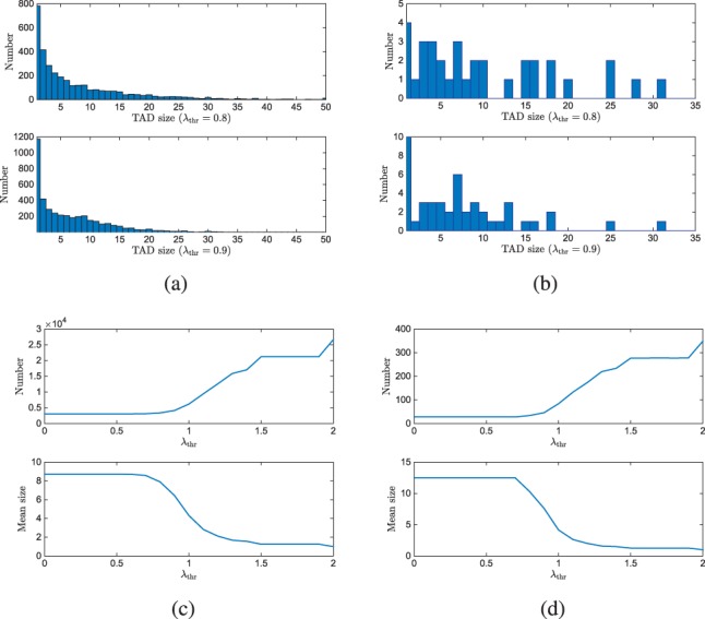
(a,b) Domain size distribution of the identified TADs on all chromosomes (a) and Chr-22 (b) with (top) and (bottom) respectively. (c,d) The number of identified TADs (top) and mean TAD size (bottom) on all chromosomes (c) and on Chr-22 (d) versus the Fiedler number threshold
Fig. 4.
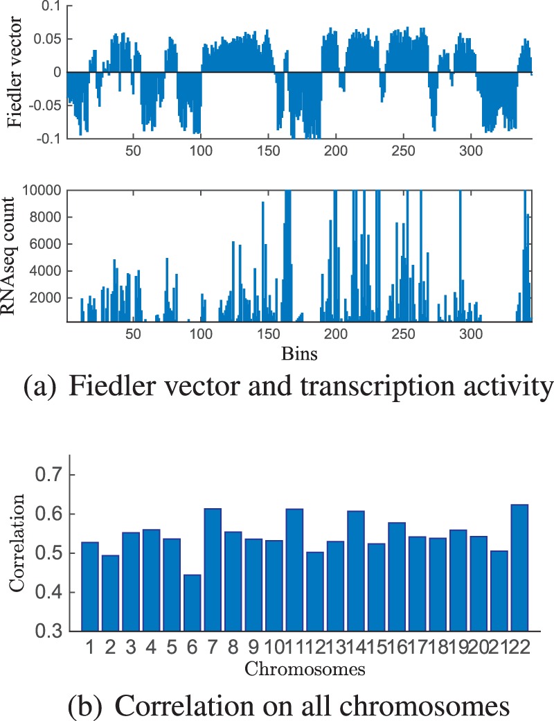
Comparison between Fiedler vector obtained in Step 1 of Algorithm 1 and transcription described by RNA-seq counts
We next illustrate the relationship between the chromosome structure and gene expression via the identified topological domains. Gene expression is represented by RNA-seq counts. RNA-seq was performed simultaneously with Hi-C in our laboratory. In order to be consistent with Hi-C matrix resolution, we summarized the gene RNA-seq counts into bins of 100 kb resolution, according to their locations. In Figure 4(a), we show the Fiedler vector of Chromosome 22 obtained in Step 1 of Algorithm 1 and its RNA-seq counts. It can be observed that the sign pattern of the Fiedler vector has high correlation with the expression levels of the RNA-seq data. Note that each locally consistent sign region is a topological domain obtained at Step 1 of Algorithm 1. To show this in a quantitive manner, we took the sign of the Fiedler vector and thresholded the RNA-seq count vector (where the threshold was selected for each chromosome to maximize the correlation), and then computed the correlation coefficient between these two vectors for all chromosomes. The correlation values are shown in Figure 4(b). Significant correlation is observed according to this result (with by permutation test. This shows that initial TADs are generally consistent with the two chromosome compartments in the genome, heterochromatin or euchromatin. We also show the decreasing trend of the relation between the averaged variance of log-scaled RNA-Seq reads within TADs versus the Fiedler number threshold (Supplementary Fig. S33). These results confirm the relationship between the identified topological domains and the functional expression (Dixon et al., 2012; Lieberman-Aiden et al., 2009), and also reveals the quality of the identified topological domain.
As compared to DP and HMM methods, the proposed method identifies TAD boundaries that are more consistent with the locations of known CTCF enrichment peaks. We plot the CTCF ChIP-seq enrichment at bins of 100 kb resolution with the locations of identified TAD boundaries for the three compared algorithms in Figure 5, with CTCF enrichment extracted from (Ziebarth et al., 2013). It has been proposed that TAD boundaries coincide with insulators such as CTCF binding sites. However, 85% of CTCF binding sites localize within TADs rather than at their borders, suggesting that most CTCF sites are unlikely to aide in identifying the borders that separate TADs. Meanwhile, multiple studies suggest that some insulator elements are not capable of enhancer-blocking or chromatin barrier activity (Schuettengruber and Cavalli, 2013; Schwartz et al., 2012; Van Bortle et al., 2012). Compared with the other two algorithms, the boundaries identified by the proposed algorithm are more consistent with CTCF enrichment peaks. A particularly visible example can be found for the large TAD between 300 and 350 bins.
Fig. 5.
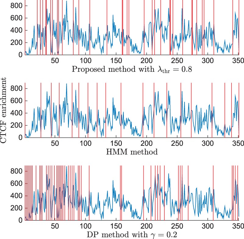
CTCF enrichment on Chromosome 22 (blue) with the locations of identified TAD boundaries (red vertical lines)
Finally, we illustrate the scalability of the proposed spectral algorithm to Hi-C data at higher resolution (5 kb) by applying it to the Hi-C IMR90 cell data of Rao et al. (2014). Results of the last 2000 bins with and are shown in Figure 6 for Chromosome 22.
Fig. 6.
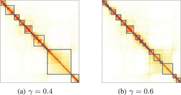
Identified topological domains on Chromosome 22 (at last 2000 bins) at resolution of 5 kb
5 Conclusion
In this paper, we presented a method for identifying topological domains based on the spectral decomposition of the graph Laplacian of the Hi-C matrix. The proposed algorithm has clear mathematical interpretation and is more computationally efficient than previous methods, allowing it to be applied to higher resolution Hi-C data. Its favorable comparison with other algorithms and its higher correlation with gene transcription dataillustrate the advantages of the proposed spectral method. Future work may include investigating fast iterative algorithms or parallel computation algorithms for improving the efficiency at higher resolutions.
Supplementary Material
Funding
This work is supported in part by the DARPA Biochronicity Program and NIH grant K25DK082791-01A109.
Conflict of Interest: none declared.
References
- Anscombe F.J. (1948) The transformation of Poisson, binomial and negative-binomial data. Biometrika, 35, 246–254. [Google Scholar]
- Anscombe F.J. (1953) Contribution of discussion paper by H. Hotelling. New light on the correlation coefficient and its transforms. J. R. Stat. Soc. B, 15, 229–230. [Google Scholar]
- Botta M. et al. (2010) Intra- and inter-chromosomal interactions correlate with CTCF binding genome wide. Mol. Syst. Biol., 6, 1–6. [DOI] [PMC free article] [PubMed] [Google Scholar]
- Boulos R.E. et al. (2013) Revealing long-range interconnected hubs in human chromatin interaction data using graph theory. Phys. Rev. Lett., 111, 118102.. [DOI] [PubMed] [Google Scholar]
- Cavalli G., Misteli T. (2013) Functional implications of genome topology. Nat. Struct. Mol. Biol., 20, 290–299. [DOI] [PMC free article] [PubMed] [Google Scholar]
- Chen H. et al. (2015a) Chromosome conformation of human fibroblasts grown in 3-dimensional spheroids. Nucleus, 6, 55–65. [DOI] [PMC free article] [PubMed] [Google Scholar]
- Chen H. et al. (2015b) Functional organization of the human 4D nucleome. Proc. Natl. Acad. Sci. (PNAS), 112, 8002–8007. [DOI] [PMC free article] [PubMed] [Google Scholar]
- Chung F.R. (1997) Spectral Graph Theory, vol. 91. American Mathematical Society.
- Dixon J.R. et al. (2012) Topological domains in mammalian genomes identified by analysis of chromatin interactions. Nature, 485, 376–380. [DOI] [PMC free article] [PubMed] [Google Scholar]
- Filippova D. et al. (2014) Identification of alternative topological domains in chromatin. Algorithms Mol. Biol., 9, 1–11. [DOI] [PMC free article] [PubMed] [Google Scholar]
- Gorkin D.U. et al. (2014) The 3D genome in transcriptional regulation and pluripotency. Cell Stem Cell, 14, 762–775. [DOI] [PMC free article] [PubMed] [Google Scholar]
- Hu M. et al. (2012) HiCNorm: removing biases in Hi-C data via Poisson regression. Bioinformatics, 28, 3131–3133. [DOI] [PMC free article] [PubMed] [Google Scholar]
- Kang U. et al. (2011) Spectral analysis for billion-scale graphs: discoveries and implementation In: Advances in Knowledge Discovery and Data Mining. Springer-Verlag Berlin Heidelberg, pp. 13–25. [Google Scholar]
- Le Dily F. et al. (2014) Distinct structural transitions of chromatin topological domains correlate with coordinated hormone-induced gene regulation. Genes Development, 28, 2151–2161. [DOI] [PMC free article] [PubMed] [Google Scholar]
- Lévy-Leduc C. et al. (2014) Two-dimensional segmentation for analyzing Hi-C data. Bioinformatics, 30, i386–i392. [DOI] [PMC free article] [PubMed] [Google Scholar]
- Lieberman-Aiden E. et al. (2009) Comprehensive mapping of long-range interactions reveals folding principles of the human genome. Science, 326, 289–293. [DOI] [PMC free article] [PubMed] [Google Scholar]
- Liu L. et al. (2012) GeSICA: Genome segmentation from intra-chromosomal association. BMC Genomics, 13, 1–10. [DOI] [PMC free article] [PubMed] [Google Scholar]
- Mesbahi M, Egerstedt M. (2010) Graph Theoretic Methods in Multiagent Networks. Princeton University Press, Princeton, NJ. [Google Scholar]
- Nora E.P. et al. (2012) Spatial partitioning of the regulatory landscape of the x-inactivation centre. Nature, 485, 381–385. [DOI] [PMC free article] [PubMed] [Google Scholar]
- Pope B.D. et al. (2014) Topologically-associating domains are stable units of replication-timing regulation. Nature, 515, 402–405. [DOI] [PMC free article] [PubMed] [Google Scholar]
- Rao S.S.P. et al. (2014) A 3D map of the human genome at kilobase resolution reveals principles of chromatin looping. Cell, 159, 1665–1680. [DOI] [PMC free article] [PubMed] [Google Scholar]
- Saad Y. (1992) Numerical Methods for Large Eigenvalue Problems. Manchester University Press, Manchester. [Google Scholar]
- Schuettengruber B., Cavalli G. (2013) Polycomb domain formation depends on short and long distance regulatory cues. PLoS One, 8, e56531.. [DOI] [PMC free article] [PubMed] [Google Scholar]
- Schwartz Y.B. et al. (2012) Nature and function of insulator protein binding sites in the drosophila genome. Genome Res., 22, 2188–2198. [DOI] [PMC free article] [PubMed] [Google Scholar]
- Sexton T. et al. (2012) Three-dimensional folding and functional organization principles of the drosophila genome. Cell, 148, 458–472. [DOI] [PubMed] [Google Scholar]
- Shi J., Malik J. (2000) Normalized cuts and image segmentation. IEEE Trans. Pattern Anal. Machine Intell., 22, 888–905. [Google Scholar]
- Van Bortle K. et al. (2012) Drosophila CTCF tandemly aligns with other insulator proteins at the borders of H3K27me3 domains. Genome Res., 22, 2176–2187. [DOI] [PMC free article] [PubMed] [Google Scholar]
- Van Bortle K. et al. (2014) Insulator function and topological domain border strength scale with architectural protein occupancy. Genome Biol., 15, R82.. [DOI] [PMC free article] [PubMed] [Google Scholar]
- Ziebarth J.D. et al. (2013) CTCFBSDB 2.0: a database for CTCF-binding sites and genome organization. Nucleic Acids Res., 41, D188–D194. [DOI] [PMC free article] [PubMed] [Google Scholar]
Associated Data
This section collects any data citations, data availability statements, or supplementary materials included in this article.