Time series analysis of influenza incidence in Chinese provinces from 2004 to 2011

Abstract

Influenza as a severe infectious disease has caused catastrophes throughout human history, and every pandemic of influenza has produced a great social burden. We compiled monthly data of influenza incidence from all provinces and autonomous regions in mainland China from January 2004 to December 2011, comprehensively evaluated and classified these data, and then randomly selected 4 provinces with higher incidence (Hebei, Gansu, Guizhou, and Hunan), 2 provinces with median incidence (Tianjin and Henan), 1 province with lower incidence (Shandong), using time series analysis to construct an ARIMA model, which is based on the monthly incidence from 2004 to 2011 as the training set. We exerted the X-12-ARIMA procedure for modeling due to the seasonality these data implied. Autocorrelation function (ACF), partial autocorrelation function (PACF), and automatic model selection were to determine the order of the model parameters. The optimal model was decided by a nonseasonal and seasonal moving average test. Finally, we applied this model to predict the monthly incidence of influenza in 2012 as the test set, and the simulated incidence was compared with the observed incidence to evaluate the model's validity by the criterion of both percentage variability in regression analyses (R²) and root mean square error (RMSE). It is conceivable that SARIMA (0,1,1)(0,1,1)₁₂ could simultaneously forecast the influenza incidence of the Hebei Province, Guizhou Province, Henan Province, and Shandong Province; SARIMA (1,0,0)(0,1,1)₁₂ could forecast the influenza incidence in Gansu Province; SARIMA (3,1,1)(0,1,1)₁₂ could forecast the influenza incidence in Tianjin City; and SARIMA (0,1,1)(0,0,1)₁₂ could forecast the influenza incidence in Hunan Province. Time series analysis is a good tool for prediction of disease incidence.

1. Introduction

Influenza viruses circulate globally and can affect all age groups, resulting in a serious public health problem. Every year, 3 to 5 million cases of severe illness and ∼250,000 to 500,000 deaths are attributed to influenza worldwide.^[1] Any outbreak of influenza could cause crushing calamity and great losses. The 1918 Spanish Flu Pandemic reportedly caused 20 to 50 million deaths.^[2] The 1957 Asia Flu and 1968 Hong Kong Flu were estimated to cause 1 million deaths or less.^[3] New subtypes of the influenza virus are emerging over time due to gradual antigen variation or antigen drift,^[4] so the influenza pandemic has never stopped and almost happens every year. The global burden of influenza epidemics on morbidity and mortality is considerable. All these bring us great suffering, presenting an urgent need to research influenza and take necessary preventive measures.

We utilize the method of time series analysis with influenza incidence data from 2004 to 2011 to construct a time series model for short-time prediction, thereby aiding as references for influenza prevention and control devoted to public health.

2. Materials and methods

2.1. Data sources

In 2004, China launched a management and surveillance information report system for infectious disease and public health emergency to significantly improve disease monitoring and early warning through network reporting. And the Chinese Center for Disease Control and Prevention (CDC) has established the National Notifiable Disease Surveillance System since then. We obtained monthly influenza incidence data from January 2004 to December 2011 in each province, including autonomous regions and municipalities in the Chinese mainland, from the National Population and Health Data Sharing Platform, which belongs to the Data center of China Public Science (http://www.phsciencedata.cn/Share/index.jsp). And the CDC, in charge of the Data center of China Public Science, has approved these data for this study.

2.2. Time series analysis

The ARIMA (p, d, q) model is extension of an autoregressive (AR) model, moving average (MA) model and ARMA model. If the data show no seasonality, the ARIMA model is perfect for forecasting. However, if there exists evident seasonality in the data, we turn to seasonal ARIMA (SARIMA) model with the X-12-ARIMA procedure. The X-12-ARIMA seasonal adjustment program is an enhanced version of X-11 Variant developed by the US Census Bureau and Statistics Canada. In the X-12 ARIMA procedure, seasonal fluctuations can be measured in the original series (Q_t, t = 1,…,n) and separated from trend-cycle, trading-day, and irregular fluctuations. The seasonal component of this time series, S_t, is the within-year variation repeated constantly or in an evolving fashion from year to year. The trend-cycle, C_t, includes fluctuations because of the long-term trend, the business cycle, and other cyclical factors. The trading-day component, D_t, is the variation attributed to the composition of calendar. The irregular component, I_t, is the residual variation that remains after the 3 components have been removed from the series.

2.3. Statical steps

There are 3 key steps involved in the ARMA modeling: identification, estimation, and diagnosis. First, we determine the need for differencing the monthly influenza incidence by checking stationarity and seasonality, and choose SARIMA model if the data show seasonality. Thus, the X-12-ARIMA procedure is used to construct the model, depicting the autocorrelation function (ACF) and partial autocorrelation function (PACF) of model residuals with different orders of both the seasonal and nonseasonal autoregressive and moving average parameters.

Second, ARMA estimates for unit root identification compares different estimated models and the best 5 ARIMA models rank these models by the Bayesian Information Criterion (BIC) value. The following parameters are selected when fitting the SARIMA (p, d, q)(P, D, Q)_s model, p refers to the order of autoregression, d is the degree of difference, and q is the order of the moving average, P stands for seasonal autoregression, D is seasonal integration, Q is seasonal moving average, and s is the length of the seasonal period.^[5] The final automatic model selection gives us the optimal model with the lowest value in BIC.^[6] Last, ACF and PACF of residuals as well as the test of nonseasonal and seasonal moving average are to evaluate the goodness of fit.

Finally, we applied this model to forecast the monthly influenza incidence from January and December 2012. To validate the model's predictive ability, data from 2004 to 2011 were used as a training set and the model fitted to only these data. The predictive ability of the model was then assessed by producing predictions for 2012 as test set and comparing the predictions made, based only on data up to 2012, to the observed values in 2012. Then a line chart for actual and predicted values was used to show the model agreement. Additionally, the predictive validity of the model was also evaluated by the criteria of root mean square error (RMSE) and percentage variability in regression analyses (R²): 

where Y_i is the observed values, ˆ Y_i is the corresponding forecasted values, and N is the number of observations. Lower RMSE values (RMSE <1) are indicative of good model performance.

For the coefficient of determination, R², the higher the R² is, the better accuracy the model indicates: 

where SSR is the sum of squared residuals, that is the sum of squared errors of prediction: 

where Y_i is the observed values, and ˆ Y_i are the forecasted values gained from the selected model. And SSY is the sum of the squared differences: 

where Y_i is the observed values, and ˆ Y_i is the mean of the observed data.

2.4. Statistical software

All analyses were performed using SAS 9.2 (SAS Statistical Institute, Cary, NC). Values of P <0.05 were regarded as significant.

3. Results

3.1. Overall incidence

Monthly influenza incidence data were collected and organized from the National Population and Health Data Sharing Platform. Figure 1 shows the average incidence from 2004 to 2011 in each province. From the histogram, we can see that most provinces fluctuate around the national average influenza incidence level. Among all the provinces in the Chinese mainland, Hebei, Ningxia, and Gansu provinces have the highest incidence, which is twice the national average. However, the incidence of influenza in northeastern China, such as the Heilongjiang, Jilin, and Liaoning provinces, is extremely low, less than one fifth of the national average.

Figure 1.

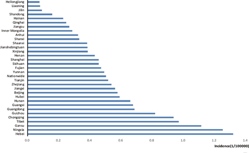
Monthly average influenza incidence (1/100,000) from 2004 to 2011 in all provinces in mainland China.

3.2. Seasonal ARIMA model

From the incidence trend nationwide (Fig. 2), the influenza incidence mostly peaks in March or September, corresponding to the common sense that influenza usually happens in winter or summer, especially during the period of seasonal exchange. The incidence sharply arises in 2008 and 2009 all the way from 2004 to 2011, which may be attributed to the H1N1 influenza pandemic in 2009.^[7] Most provinces keep consistent with the national trend.

Figure 2.

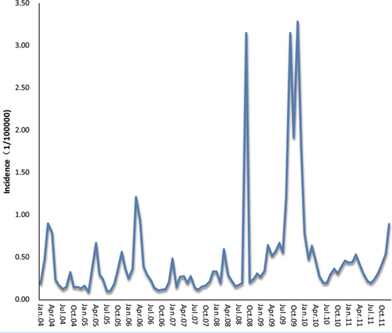
Monthly influenza incidence (1/100,000) nationwide in mainland China from January 2004 to December 2011.

Different provinces may have different models in accordance with the monthly incidence data, we just randomly chose 4 provinces with higher influenza incidence—Hebei Province, Gansu Province, Guizhou Province, and Hunan Province—2 provinces with median incidence—Henan Province and Tianjin City—1 province with lower incidence—Shangdong Province as examples. Here, we took the Hebei Province with the highest average incidence over these years as representative for modeling and forecasting. As with the seasonality, the monthly influenza incidence time series data from January 2004 to December 2011 in Hebei Province exhibits (Fig. 3), the X-12-ARIMA procedure is performed to construct the seasonal ARIMA model. Autocorrelation functions (ACF) and partial autocorrelation functions (PACF) of model residuals at different nonseasonal and seasonal differencing indicate that when diff=1 and sdiff=1, ACF and PACF are stationary, and PACF attenuates to zero slowly as well (Fig. 4). So we can preliminarily assume the fit model is (0,1,1)(0,1,1)₁₂. At the same time, the automatic model identification is also (0,1,1)(0,1,1). We may determine that the appropriate model could be SARIMA(0,1,1)(0,1,1)₁₂. Furthermore, nonseasonal and seasonal moving average test both reject the null hypothesis (P < 0.05) with lowest BIC (Table 1), suggesting that the model is suitable. Moreover, the spectrum plot for incidence by X-12-ARIMA step by step confirms this model. Three seasonal peaks are found in the spectral plot for original data (Fig. 5A). Visually significant residual peaks have been found in the spectral plot of the differenced, transformed original series starting in January 2004 (Fig. 5B). When it turns to the spectrum plot for the differenced, transformed seasonally adjusted data, and the modified irregular data, the seasonal frequency becomes weaken (Fig. 5C and D), eliminating the seasonal impact to the model. Lastly, to validate the model's predictive ability, we used the constructed model SARIMA (0,1,1)(0,1,1)₁₂ to predict the monthly incidence in 2012 and then compared the observed values with the predicted values. The model fitted the data reasonably well (Fig. 6) with low RMSE (0.0625) and high R² (0.9425). It showed that the parsimonious model SARIMA (0,1,1)(0,1,1)₁₂ was appropriate for forecasting influenza incidence in Hebei Province.

Figure 3.

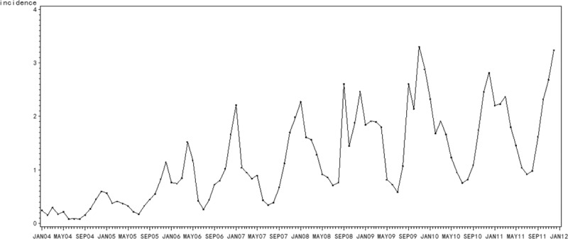
Time series for monthly influenza incidence (1/100,000) in the Hebei Province from January 2004 to December 2011.

Figure 4.

Autocorrelation functions (ACF) and partial autocorrelation functions (PACF) of model residuals at different nonseasonal and seasonal differencing for monthly influenza incidence from January 2004 to December 2011 in the Hebei Province: (A) nonseasonal difference = 0, seasonal difference = 0; (B) nonseasonal difference = 0, seasonal difference = 1; (C) nonseasonal difference = 1, seasonal difference = 0; (D) nonseasonal difference = 1, seasonal difference = 1.ACF, autocorrelation functions, PACF = partial autocorrelation functions.

Table 1.

Coefficients of the seasonal ARIMA model on the monthly influenza incidence in mainland China, 2004–2011.

Figure 5.

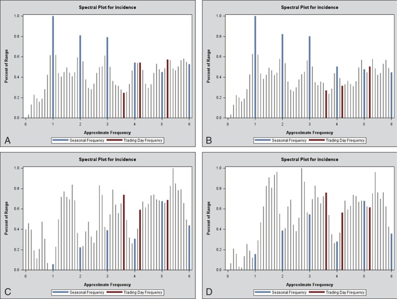
Spectrum plot for monthly influenza incidence (1/100,000) from 2004 to 2011 in the Hebei Province by the X-12-ARIMA procedure: (A) spectral plot for original data; (B) spectral plot of the differenced, transformed original series; (C) spectrum plot for the differenced, transformed seasonally adjusted data; (D) spectrum plot for the modified irregular data. ARIMA = autoregressive integrated moving average.

Figure 6.

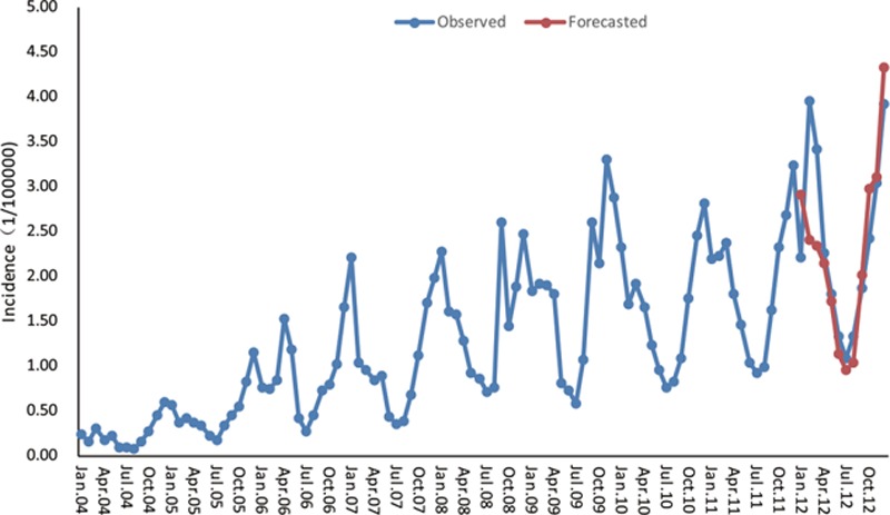
SARIMA (0,1,1)(0,1,1)₁₂-fitted influenza time series (Jan. 2004–Dec. 2011) and forecasted incidence (Jan. 2012–Dec. 2012) in the Hebei Province. The blue dotted line represents the observed values of influenza incidence from 2004 to 2012, and the red dotted line represents the SARIMA (0,1,1)(0,1,1)₁₂ model's fitted curve of 2012. SARIMA = seasonal autoregressive integrated moving average.

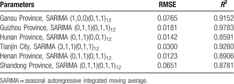
We also construct a SARIMA model for another 3 selected provinces with high influenza incidence, 2 provinces with median incidence, and 1 province with lower incidence by seasonal ARIMA modeling as the Hebei Province. SARIMA (1,0,0)(0,1,1)₁₂ is suitable for Gansu Province (RMSE = 0.0765, R² = 0.9152); SARIMA (0,1,1)(0,1,1)₁₂ is good for Guizhou Province (RMSE = 0.0181, R² = 0.9783); SARIMA (0,1,1)(0,0,1)₁₂ is fit for Hunan Province (RMSE = 0.0142, R² = 0.8591); SARIMA (3,1,1)(0,1,1)₁₂ is appropriate for Tianjin City (RMSE = 0.0300, R² = 0.9280); SARIMA (0,1,1)(0,1,1)₁₂ is suitable for Henan Province (RMSE = 0.0123, R² = 0.8906); SARIMA (0,1,1)(0,1,1)₁₂ is proper for Shandong Province (RMSE = 0.0651, R² = 0.8781) (Fig. 7A–F, Table 2).

Figure 7.

SARIMA (p,d,q)(P,D,Q)_s-fitted influenza time series (Jan. 2004–Dec. 2011) and forecasted incidence (Jan. 2012–Dec. 2012) in different Provinces/Cities. The blue dotted line represents the observed values of influenza incidence from 2004 to 2012, and the red dotted line represents the constructed model's fitted curve of 2012. SARIMA (p,d,q)(P,D,Q)_s can be used for the short-term forecast of the influenza incidence. (A) SARIMA (1,0,0)(0,1,1)₁₂-fitted influenza time series (Jan. 2004–Dec. 2011) and forecasted incidence (Jan. 2012–Dec. 2012) in the Gansu Province. (B) SARIMA (0,1,1)(0,1,1)₁₂-fitted influenza time series (Jan. 2004–Dec. 2011) and forecasted incidence (Jan. 2012–Dec. 2012) in the Guizhou Province. (C) SARIMA (0,1,1)(0,0,1)₁₂-fitted influenza time series (Jan. 2004–Dec. 2011) and forecasted incidence (Jan. 2012–Dec. 2012) in the Hunan Province. (D) SARIMA (3,1,1)(0,1,1)₁₂-fitted influenza time series (Jan. 2004–Dec. 2011) and forecasted incidence (Jan. 2012–Dec. 2012) in the Tianjin City. (E) SARIMA (0,1,1)(0,1,1)₁₂-fitted influenza time series (Jan. 2004–Dec. 2011) and forecasted incidence (Jan. 2012–Dec. 2012) in the Henan Province. (F) SARIMA (0,1,1)(0,1,1)₁₂-fitted influenza time series (Jan. 2004–Dec. 2011) and forecasted incidence (Jan. 2012–Dec. 2012) in the Shandong Province. SARIMA = seasonal autoregressive integrated moving average.

Table 2.

Statistical validation of SARIMA models.

4. Discussion

Influenza is related to every one of us, including males, females, the old, and the young. The influenza virus mutates easily and quickly, resulting in an influenza pandemic every year. This leads to significant medical consumption and social burden. China, as a vast and populous country, has already carried out many preventive policies and established a health surveillance system. In spite of these measures, influenza still prevails. There are many factors that affect influenza incidence, including virus virulence, the environment, geographical location, population mobility, preventive strategies, economic status, and so on.^[8] We cannot inhibit or eliminate the virus, but we can prevent it or minimize the loss when the disease occurs. In this study, we introduced and used statistical methods that have been rarely used in influenza forecasts to construct models for predicting influenza incidence, thus providing research ideas for influenza prevention and aiding guidance for public health.

As a traditional public health affair, epidemiology surveillance of infectious diseases is pervasive, and model forecasting will better utilize the surveillance data.^[9,10] It has been proven that statistical models are helpful in predicting future communicable disease incidence, and it is crucial for the hygiene department to recognize epidemic behavior earlier.^[11] The autoregressive integrated moving average (ARIMA) model of time series analysis was originally conceived for economics but has been widely used in the community of infectious disease for numbers of different time varying events. ARIMA is very useful to fit time-series data and has been exhibited to be the most successful approach to model a variety of time series.^[12,13] Time series models play a significant role in disease prediction, as they can predict the future occurrence of disease with incidence data collected monthly or yearly.^[14] They have been used for the prediction of influenza mortality,^[15,16] malaria incidence,^[17,18] hemorrhagic fever with renal syndrome (HFRS) incidence,^[19] and other infectious diseases.^[9,20,21] They have also been applied in exploring the relationship between changes in national alcohol policies and suicide incidence,^[22] the relationship between leptospirosis and temperature and rainfall,^[23] and so on.

The ARIMA (Box-Jenkins) methodology has been increasingly applied in medical fields,^[15,24–29] and the ARIMA model has been confirmed as an application to predict infectious disease trends. But if the data presents seasonality, the X-12-ARIMA procedure is used to construct a seasonal ARIMA model.^[30] The national influenza incidence shows obvious seasonality and fluctuation (Fig. 2). Influenza cases (exceeding approximately average 75,000 cases every year) have been reported by the National Notifiable Disease Surveillance System.^[31] The Chinese National Notifiable Disease Surveillance System has already covered 100% CDC nationwide with a reporting rate of 100%, 98% county medical establishments or the above with a reporting rate of 95.99%, 88% township and village health centers with a reporting rate of 83.92%.^[32,33] Notification rates are known to have improved from 2005, when China established a national influenza-like illness (ILI) surveillance system in 2005 and laboratory reporting became mandatory,^[34] which partially explains the subsequent increase in cases from this time onwards (Figs. 2 and 3). Influenza, unlike other infectious disease, as a lipid-enveloped, air-borne virus, exhibits obvious and robust seasonality.^[35] Studies have illustrated that a regular winter pattern is noted for northern China and clear peaks in summer as well as less pronounced peaks in winter are common in southern China, which are regular epidemic phenomena and trends for seasonal influenza in China,^[36–38] consistent with the typical seasonal pattern in the Northern Hemisphere and Southern Hemisphere, respectively.^[39] Taking the seasonal pattern together with representative sample of influenza demonstrated above into consideration, the time series data in this study could reflect and represent the seasonality and general trends of influenza despite the reporting biases.

Here, we selected the Hebei Province as an example to construct a model with the monthly influenza incidence from January 2004 to December 2011—training set (Figs. 3–Fig. 5). Then, we predicted the monthly incidence in 2012 with the model test set, compared the predicted value with actual value, and concluded that the 2 sets of data agreed closely (Fig. 6). With the good predictive ability, the model is able to make reasonable future predictions based on past data. Therefore, SARIMA (0,1,1)(0,1,1)₁₂ is effective in forecasting the influenza incidence of the Hebei province, and the model could be valuable to prevent and control influenza. If the forecasted incidence is to increase, more policies or improved measures such as health propagandization, personal protection, and protective vaccines could be taken ahead of time to minimize the loss as much as possible. For the other provinces, the same modeling process as the 1 procedure in the Hebei Province will be used to construct the optimal prediction model. From the fitted ARIMA model of the higher influenza incidence provinces—the Gansu Province, the Guizhou Province, and the Hunan province—the median incidence provinces—the Tianjin City and the Henan Province—the lower incidence province—the Shandong Province (Fig. 7, Table 2), it turns out that the SARIMA model can effectively predict the influenza incidence in the future.

It is big data era now, massive data are emerging everyday permeating into almost every facet of our lives, and how to exert the data in public health is of great importance in disease prevention and control.^[40] Time series analysis of infection data is useful to propose new hypotheses, anticipate epidemic trends, and improve the prevention system. This study constructs a seasonal ARIMA model to forecast influenza incidence, contributing to an early warning system that can help public health policy makers take measures to prevent it from spreading, improve public awareness, and reallocate resources. This statistical method suggested in this study does a lot to benefit public health.

However, there are also some limitations of our study. The SARIMA model is only used for short-term forecasting, and it may not be so robust or accurate for long-term forecasting. Continuous surveillance and monitoring are indispensable. We should dynamically adjust the model by adding new monitoring data for influenza incidence. It is promising that, with more reliable influenza data and further model refinement, these seasonal ARIMA models by time series analysis method could facilitate more sufficient references for public officials to prepare for influenza epidemics.

References

- 1.Word Health Organization (WHO) media centre (http://www.who.int/mediacentre/factsh eets/fs211/en/) Accessed March 2014. [Google Scholar]
- 2.Johnson NP, Mueller J. Updating the accounts: global mortality of the 1918–1920 “Spanish” influenza pandemic. Bull Hist Med 2002; 76:105–115. [DOI] [PubMed] [Google Scholar]
- 3.Nguyen-Van-Tam JS, Hampson AW. The epidemiology and clinical impact of pandemic influenza. Vaccine 2003; 21:1762–1768. [DOI] [PubMed] [Google Scholar]
- 4.Alonso WJ, Vibound C, Simonsen L, et al. Seasonality of influenza in Brazil: a traveling wave from the Amazon to the subtropics. Am J Epidemiol 2007; 165:1434–1442. [DOI] [PubMed] [Google Scholar]
- 5.Box GE, Jekins GM, Reinsel GC. Time Series Analysis: Forecasting and Control. 4th edn. 2008; New Jersey: John Wiley & Sons, 645–660. [Google Scholar]
- 6.Wang Y. Applied Time Series Analysis. 3rd edn. 2012; Beijing: People's University of China, 103–201. [Google Scholar]
- 7.Bellido-Blasco JB, Pardo-Serrano F, Ballester-Rddriguez I, et al. An estimate of the incidence of influenza-like illness during the influenza pandemic of 2009. Arch Bronconeumol 2015; 51:373–378. [DOI] [PubMed] [Google Scholar]
- 8.Yin JK, Salkeld G, Heron L, et al. The threat of human influenza: the viruses, disease impacts, and vaccine solutions. Infect Disord Drug Targets 2014; 14:150–154. [DOI] [PubMed] [Google Scholar]
- 9.Liu Q, Liu X, Jiang B, et al. Forecasting incidence of hemorrhagic fever with renal syndrome in China using ARIMA model. BMC Infec Dis 2011; 11:218. [DOI] [PMC free article] [PubMed] [Google Scholar]
- 10.Nsubuga P, White ME, Thacker SB. Jamison DT, et al. Public health surveillance: a tool for targeting and monitoring interventions. Disease Control Priorities in Developing Countries 2nd ed.Washington DC: World Blank; 2006. 997–1015. [Google Scholar]
- 11.Earnest A, Chen MI, Ng D, et al. Using autoregressive integrated moving average (ARIMA) models to predict and monitor the number of beds occupied during a SARS outbreak in a tertiary hospital in Singapore. BMC Health Serv Res 2005; 5:36. [DOI] [PMC free article] [PubMed] [Google Scholar]
- 12.Garcia-Diaz JC. Monitoring and forecasting nitrate concentration in the groundwater using statistical process control and time series analysis: a case study. Stoch Environ Res Risk Assess 2011; 25:331–339. [Google Scholar]
- 13.McGee VE, Jenkins E, Rawnsley HM. Statistical forecasting in a hospital clinical laboratory. J Med Syst 1979; 3:161–174. [DOI] [PubMed] [Google Scholar]
- 14.Kane MJ, Prince N, Scotch M, et al. Comparison of ARIMA and Random Forest time series models for prediction of avian influenza H5N1 outbreaks. BMC Bioinformatics 2014; 15:276. [DOI] [PMC free article] [PubMed] [Google Scholar]
- 15.Reichert TA, Simonsen L, Sharma A, et al. Influenza and the winter increase in mortality in the United States, 1959–1999. Am J Epidemiol 2004; 160:492–502. [DOI] [PubMed] [Google Scholar]
- 16.Dominguez A, Munoz P, Martine A, et al. Monitoring mortality as an indicator of influenza in Catalonia, Spain. J Epidemiol Community Health 1996; 50:293–298. [DOI] [PMC free article] [PubMed] [Google Scholar]
- 17.Gaudart J, Toure O, Dessay N, et al. Modelling malaria incidence with environmental dependency in a locality of Sudanese savannah area, Mali. Malar J 2009; 8:61. [DOI] [PMC free article] [PubMed] [Google Scholar]
- 18.Hanf M, Adenis A, Nacher M, et al. The role of El Nino Southern Oscillation (ENSO) on variations of monthly Plasmodium falciparum malaria cases at the Cayenne General Hospital, 1996–2009, French Guiana. Malar J 2011; 10:100. [DOI] [PMC free article] [PubMed] [Google Scholar]
- 19.Liu Q, Liu X, Jiang B, et al. Forecasting incidence of hemorrhagic fever with renal syndrome in China using ARIMA model. BMC Infect Dis 2011; 11:218. [DOI] [PMC free article] [PubMed] [Google Scholar]
- 20.Luz PM, Mendes BV, Codeco CT, et al. Time series analysis of dengue incidence in Rio de Janeiro, Brazil. Am J Trop Med Hyg 2008; 79:933–939. [PubMed] [Google Scholar]
- 21.Yi J, Du CT, Wang RH, et al. Applications of multiple seasonal autoregressive integrated moving average (ARIMA) model on predictive incidence of tuberculosis. Chin J Prev Med 2007; 41:118–121. [PubMed] [Google Scholar]
- 22.Pridemore WA, Snowden AJ. Reduction in suicide mortality following a new national alcohol policy in Slovenia: an interrupted time-series analysis. Am J Public Health 2009; 99:915–920. [DOI] [PMC free article] [PubMed] [Google Scholar]
- 23.Chadsuthi S, Modchang C, Lenbury Y, et al. Modeling seasonal leptospirosis transmission and its association with rainfall and temperature in Thailand using time-series and ARIMA analyses. Asian Pac J Trop Med 2012; 5:539–546. [DOI] [PubMed] [Google Scholar]
- 24.Ramirez AP, Buitrago JI, Gonzalez JP, et al. Frequency and tendency of malaria in Colombia, 1990 to 2011: a descriptive study. Malar J 2014; 13:202. [DOI] [PMC free article] [PubMed] [Google Scholar]
- 25.Tang F, Cheng Y, Bao C, et al. Spatio-temporal trends and risk factors for Shigella from 2001 to 2011 in Jiangsu Province, People's Republic of China. PloS One 2014; 9:e83487. [DOI] [PMC free article] [PubMed] [Google Scholar]
- 26.Wakefield MA, Coomber K, Durkin SJ, et al. Time series analysis of the impact of tobacco control policies on smoking prevalence among Australian adults, 2001–2011. Bull World Health Organ 2014; 92:413–422. [DOI] [PMC free article] [PubMed] [Google Scholar]
- 27.Kadri F, Harrou F, Chaabane S, et al. Time series modelling and forecasting of emergency department overcrowding. J Med Syst 2014; 38:107. [DOI] [PubMed] [Google Scholar]
- 28.Yang L, Bi ZW, Kou ZQ, et al. Time-series analysis on human brucellosis during 2004–2013 in Shandong province, China. Zoonoses Public Health 2015; 62:228–235. [DOI] [PubMed] [Google Scholar]
- 29.Yu HK, Kim NY, Kin SS, et al. Forecasting the number of human immunodeficiency virus infections in the korean population using the autoregressive integrated moving average model. Osong Public Health Res Perspect 2013; 4:358–362. [DOI] [PMC free article] [PubMed] [Google Scholar]
- 30.Li XX, Wang LX, Zhang H, et al. Seasonal variations in notification of active tuberculosis cases in China, 2005–2012. PLoS One 2013; 8:e68102. [DOI] [PMC free article] [PubMed] [Google Scholar]
- 31.The Data-center of China Public Health Science (http:/http://www.phsciencedata.cn/Share/en/index.jsp). [Google Scholar]
- 32.Ji YB, Guo Y, Guo Q, et al. Sample survey of the legal infectious disease monitoring report management in 2008. Chin J Dis Control Prev 2011; 15:141–144. [Google Scholar]
- 33.Chinese Center for Disease Control and Prevention. (http://www.chinacdc.cn/zxdt/201203/t20120316_58667.htm) Accessed 16 Mar 2012. [In Chinese]. [Google Scholar]
- 34.Peng Z, Feng L, Carolyn GM, et al. Characterizing the epidemiology, virology, and clinical features of influenza in China's first severe acute respiratory infection sentinel surveillance system, February 2011–October 2003. BMC Infect Dis 2015; 15:143. [DOI] [PMC free article] [PubMed] [Google Scholar]
- 35.Charland KM, Buckeridge DL, Sturtevant JL, et al. Effect of environmental factors on the spatio-temporal patterns of influenza spread. Epidemiol Infect 2009; 137:1377–1387. [DOI] [PubMed] [Google Scholar]
- 36.Shu YL, Fang LQ, de Vlas SJ, et al. Dual seasonal patterns for influenza, China. Emerg Infect Dis 2010; 16:725–726. [DOI] [PMC free article] [PubMed] [Google Scholar]
- 37.Gao Y, Fang LQ, Zhang Y, et al. Spatiotemporal characteristics of seasonal influenza in mainland China. Zhonghua Liu Xing Bing Xue Za Zhi 2009; 30:1097–1101. [PubMed] [Google Scholar]
- 38.Zhang J, Yang WZ, Guo YJ, et al. Epidemiologic characteristics of influenza in China, from 2001 to 2003. Zhonghua Liu Xing Bing Xue Za Zhi 2004; 25:461–465. [PubMed] [Google Scholar]
- 39.Tang JW, Lai FY, Nymadawa P, et al. Comparison of the incidence of influenza in relation to climate factors during 2000–2007 in five countries. J Med Viro 2010; 82:1958–1965. [DOI] [PubMed] [Google Scholar]
- 40.Ma JQ. Big data application in public heath. Chin J Health Inform Manag 2014; 11:174–181. [Google Scholar]