Automated detection and analysis of depolarization events in human cardiomyocytes using MaDEC

Abstract

Optical imaging-based methods for assessing the membrane electrophysiology of in vitro human cardiac cells allow for non-invasive temporal assessment of the effect of drugs and other stimuli. Automated methods for detecting and analyzing the depolarization events (DEs) in image-based data allow quantitative assessment of these different treatments. In this study, we use 2-photon microscopy of fluorescent voltage-sensitive dyes (VSDs) to capture the membrane voltage of actively beating human induced pluripotent stem cell-derived cardiomyocytes (hiPS-CMs). We built a custom and freely available Matlab software, called MaDEC, to detect, quantify, and compare DEs of hiPS-CMs treated with the β-adrenergic drugs, propranolol and isoproterenol. The efficacy of our software is quantified by comparing detection results against manual DE detection by expert analysts, and comparing DE analysis results to known drug-induced electrophysiological effects. The software accurately detected DEs with true positive rates of 98–100% and false positive rates of 1–2%, at signal-to-noise ratios (SNRs) of 5 and above. The MaDEC software was also able to distinguish control DEs from drug-treated DEs both immediately as well as 10 min after drug administration.

1. Introduction

The derivation of human induced pluripotent stem cells (hiPS) from somatic human cells has opened broad opportunities in the study of human cardiac cells. Previously limited by their minimal proliferation, human cardiomyocytes were difficult to obtain in significant number to allow widespread study. hiPS cells can be expanded into the required quantities and then differentiated into cardiomyocytes (hiPS-CM) as a new, and seemingly endless, source of cardiomyocytes [18, 30]. Accompanying this expanded availability, there has been an acceleration of the development of new methods for assessing the electrophysiological effects of drug compounds. Image-based tools for assessing excitable cells, such as cardiomyocytes, have particularly come to the fore [3, 5, 14, 22, 25, 27]. With these new data acquisition methods comes a need for automated, user friendly, analysis methods of these image-based data.

Voltage-sensitive dyes (VSD) are one such method for acquiring membrane voltage data. These dyes associate with cellular membranes and exhibit a characteristic increase in fluorescence intensity proportional to an increase in voltage across the membrane. This allows for non-invasive, non-destructive, and longitudinal assessment of hiPS-CM electrophysiology [11, 29]. VSDs have previously been used in neuronal [8, 21] and cardiac [7, 10, 15] cells and tissues. A wide range of VSD compounds and properties have been synthesized [29]. This study utilizes di-4-ANE(F)PPTEA, a hemicyanine class dye, to acquire a temporal fluorescent signal that corresponds to the changing voltage of hiPS-CM membranes.

To quantitatively assess these data acquired using VSDs in hiPS-CM, we built a custom Matlab software (MaDEC), capable of both detecting and analyzing individual VSD depolarization waveforms or depolarization events (DEs). Our previous work has analyzed hiPS-CM electrophysiology by performing supervised machine learning on predefined DE parameters [11] of already detected DEs. Here, detection is performed using a generalized matched filter for the entire waveform instead. This allows for non-biased event selection, as well as more reliable event selection in low-SNR environments. This detection method was previously shown to be successful for neuronal action potential detection in extracellularly recorded micro-electrode data [23], as well as neuronal calcium transient wave detection in calcium imaging data [24]. The detected DEs are subsequently compared, using a K-S test, across treatments and time points. The chronotropic drugs propranolol and isoproterenol were selected to validate this VSD-based approach and the corresponding analysis software. This method of analysis allows for quantitative assessment of the heterogeneity of DEs at a precise location on the membrane of an actively beating cardiomyocyte. Furthermore, this method allows quantitative assessment of how a given drug affects the DE shape of an actively beating cardiomyocyte.

In this study, we use 2-photon microscopy of fluorescent VSD to assess the depolarization of the cell membrane voltage of actively beating hiPS-CM. Using MaDEC, we detect, quantify, and compare DEs of hiPS-CMs treated with common β-adrenergic drugs. The efficacy of our software is quantified by comparing detection results against manual DE detection by expert analysts, and comparing DE analysis results to known drug induced electrophysiological effects.

2. Methods

2.1. Human Induced Pluripotent Stem Cell-Derived Cardiomyocyte (hiPS-CM) Culture and Differentiation

hiPS-CMs were prepared for interrogation per the protocol previously described by Heylman, et. al [11]. Briefly, wtc11 hiPS cells were differentiated into cardiomyocytes using a serum-free defined medium protocol [16]. Cells began spontaneously beating on approximately Days 12–15, and were stained with VSD and imaged on Day 33.

2.2. Voltage-Sensitive Dye Staining and Drug Exposure

Culture medium was replaced with fresh medium containing 1μM Di-4-ANE(F)PPTEA (purchased from Leslie Loew, University of Connecticut) and incubated for 15 min at 37°C. Cells were rinsed with RPMI/B-27 (+) insulin one time and then allowed to recover for at least 2 hours prior to imaging. After staining with VSD, cells were qualitatively confirmed to still be spontaneously beating before addition of drugs. Medium was then replaced with fresh medium containing either 10⁻⁵μM propranolol (SIGMA, P0884) or 10⁻⁷μM isoproterenol (SIGMA, I6504). Data was collected immediately after addition of drugs (less than 60 sec of exposure) and again 10 min or 15 min after addition to ensure complete exposure. Control images were captured from VSD stained cultures, not treated with either drug.

2.3. Two-Photon Microscopy

A Zeiss LSM 710 microscope (Carl Zeiss, Jena, Germany) with a 40× water immersion objective (C-Apochromat 40X/1.20 W Korr M27) was used for all measurements. VSD was excited by an 850nm light produced by a titanium:sapphire Mai Tai laser (Spectra-Physics, Mountain View, CA). Excitation light was separated from emission signal with a 760nm dichroic. VSD fluorescence was collected in the 489–645 nm range. Line scan mode with 128 pixels per line and a 1.58 μs pixel dwell time was used to acquire temporal VSD depolarization data. Given a 1.67 kHz sampling rate, the total scan time per line was 600 μs. Each measurement consisted of 100,000 line scan repeats (total scan time 60 s). The Zen software package (Zeiss, Jena, Germany) was used to control all microscope components and acquisition processes. Brightfield images were used to identify clusters of spontaneously beating cardiomyocytes. The system was then switched to line scan mode with the parameters specified above. Line scan data were acquired along a line that was manually drawn across cell membranes. After completion of data acquisition, the system was switched back to brightfield mode to confirm that the cells were still spontaneously beating.

2.4. Data Pre-Processing

SimFCS commercial software developed in the Laboratory of Fluorescence Dynamics (LFD, University of California, Irvine) was used to analyze raw fluorescence data. A Gaussian tracking and correction algorithm (Supplemental Fig. 6) was used to compensate for motion artifacts resulting from the spontaneous beating of cell clusters. Fluorescence intensity along each corrected cell membrane trace was then extracted. Finally, a custom Matlab script that fit and subtracted a biexponential function from the resultant data was used to remove photobleaching artifacts (Supplemental Fig. 7).

2.5. Manual Identification of Depolarization Event

Intensity traces, X, for all drug and control conditions, as described in Sec. 2.2, were derived as described in Sec. 2.4, and plotted in Matlab. Three trained human analysts then independently identified DE peak times from each trace.

2.6. DE Detection and Comparison Analysis (MaDEC)

We have designed a custom Matlab software package to detect, quantify, and compare DEs of hiPS-CMs treated with common β-adrenergic drugs. The package consists of two components. First, the DEs are detected using a Matched-filter for Depolarization Event (MaD) detection. The detected DEs are then quantitatively compared using our DE Comparison tool (DEC). Combined, these two tools are referred to as MaDEC. MaDEC was implemented in Matlab and is freely available along with a graphical user interface at sites.uci.edu/aggies/downloads or from the corresponding author.

2.6.1. Matched-filter for Depolarization Event Detection (MaD)

The matched filter used here was first implemented in Szymanska et al. [24]. A few modifications were made to tailor the filter specifically to voltage-sensitive dye and cardiomyocyte data, resulting in the MaD detector. Briefly, given a fluorescence intensity signal $x\in {ℝ}^{1\times N}$, where N is the number of samples spanning a DE, and assuming Gaussian noise statistics, we can express a decision rule as

$$\begin{array}{c}\text{accept}{H}_0\text{if}S\left(x\right)<\gamma \\ \text{accept}{H}_1\text{if}S\left(x\right)>\gamma \end{array},\text{where}S(x)=s{\displaystyle {\sum }^{-1}}{x}^T$$ (1)

is the test statistic and matched-filter output, $s\in {ℝ}^{1\times N}$ is the DE template, $\sum \in {ℝ}^{N\times N}$ is the noise covariance matrix, γ is the threshold, H₀ is the null hypothesis (the signal contains noise only), and H₁ is the alternative hypothesis (the signal contains both noise and a DE). To detect DEs in the entire line scan, the matched filter is convolved with the full line scan signal $X\in {ℝ}^{1\times T}$, where T ≫ N, and DEs are identified as peaks of activity above the threshold, γ.

MaD Detector Training Protocol

The MaD detector is completely data driven as both s and Σ from Eq. 1 are estimated from the data. This allows the detector to be very flexible in accommodating various DE sizes, shapes, and durations, depending on the drug treatment applied and the specific data collected. The detector was trained under three detection conditions. The first was no drug exposure (control); the second was isoproterenol exposure and included data immediately after and 10 min after addition of isoproterenol; the third was propranolol exposure and included data immediately after and 10 min after addition of propranolol. The appropriately trained detector was then used to extract DEs from the data.

In order to estimate s and Σ, 20 high-SNR DEs (N = 800 ≃ 0.48 s), as well as 20 noise-only data samples, were identified manually for each detection condition. Analysts identified between 81 and 142 DEs in the control data, depending on the analyst (Table 2). Therefore, the 20 control training DEs represent 14–25% of the total control DEs. Similarly, the 20 isoproterenol training DEs represent 15–16% of the total isoproterenol DEs, and the 20 propranolol training DEs represent 24% of the total propranolol DEs. These training DEs were then aligned to their peak values, and averaged to construct s for each detection condition. The identified training noise samples were subdivided into windows (N = 800 ≃ 0.48 s), and auto-covariance sequences, r(k), were then calculated at lags k ∈ {−399, −398, ⋯, 399} for each noise window. The total available noise in each detection condition is difficult to quantify, however we can present the training noise for each detection condition in terms of a percentage of the full data for that detection condition. The training noise samples in the control condition, isoproterenol condition, and propranolol condition represent 14%, 7%, and 15% of the control, isoproterenol, and propranolol data, respectively. The Σ for each detection condition was generated by averaging the auto-covariance sequences across that detection condition’s noise windows.

Table 2.

Number and average SNRs of manually identified DEs for each analyst and each data trace. The last column shows the number and average SNR of DEs unanimous among all 3 analysts. The percentage agreement between each analyst and the unanimous DEs is also shown.

Treatment		Analyst				Unanimous DEs
		1	2	3	Average
Control-1	# DEs	60	59	60	59.67	59
	Avg. SNR	5.64	5.71	5.64	5.67	5.71
	Agreement (%)	98.31	100	98.31	98.87
Control-2	# DEs	81	142	94	105.67	76
	Avg. SNR	3.12	2.91	3.18	3.07	3.19
	Agreement (%)	92.18	53.52	80.85	75.52
Iso-1	0 min (# DEs)	63	63	62	62.75	62
	10 min (# DEs)	66	67	67	66.50	66
	Avg. SNR	69.76	69.32	70.15	69.74	70.58
	Agreement (%)	99.22	98.46	99.22	99.03
Iso-2	15 min (# DEs)	43	107	46	65.33	38
	Avg. SNR	0.70	0.58	0.61	0.63	0.65
	Agreement (%)	88.37	35.51	82.61	68.83
Pro-1	0 min (# DEs)	55	55	55	55	55
	10 min (# DEs)	29	29	29	29	29
	Avg. SNR	30.97	30.97	30.97	30.97	30.97
	Agreement (%)	100.00	100.00	100.00	100.00

The size of s and each noise window was empirically selected as N = 800 ≃ 0.48 s to ensure that most DEs were captured in full, although some data sets did exhibit both wider and slimmer DEs depending on the drug treatment. The number of noise windows for a given drug treatment varied depending on the length of available noise-only segments in the pre-processed data. Likewise, the shape and SNR of DEs used for estimating s varied between drug treatments. Examples of s from both propranolol and isoproterenol drug treatments, as well as the control, are shown in Fig. 1. The average SNR of the training DEs, as well as the number of training noise windows available for each drug treatment is listed in Table 1.

Figure 1.

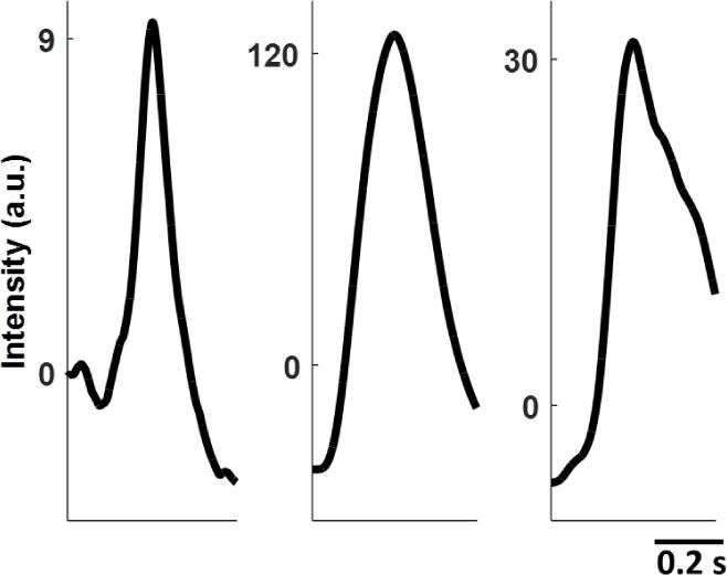
Examples of training templates s from control (left), isoproterenol (middle), and propranolol (right) data. Each template is 0.48 s long.

Table 1.

Training sample information for each drug treatment. Average training DE SNR is the average SNR of the 20 DEs selected for training for a given drug treatment. The number of windows the training noise sample for each data set could be split into is also listed.

Training Condition	Average Training DE SNR	Number of Training Noise Windows
Control	3.77	34
Isoproterenol	148.07	17
Propranolol	158.97	37

2.6.2. DE Comparison (DEC) Analysis

Once the DEs were detected from each data trace, the individual spikes were extracted from the data and normalized such that the average DE for any given data trace had a minimum value of 0 and a maximum value of 1. This approach allowed us to preserve within data trace variations around the average DE, while also normalizing DE amplitudes across different data traces. We chose to normalize the DEs because their amplitudes are highly dependent on photobleaching, exact position in the imaging plane, as well as how much of the VSD each membrane initially absorbed. It is therefore unreliable to compare DE amplitudes across treatments and time. Each DE was defined by a window consisting of 800 time points (≃0.48 s) centered on the maximum value of the DE. The average waveforms were calculated for each data trace. The full-width half-max (width), the positive slope at half-max (upslope), and the negative slope at half-max (downslope) were calculated for each identified DE. These parameters were compared as a function of drug treatment and time elapsed after drug treatment using a two-sample Kolmogorov-Smirnov (K-S) test at a 5% significance level.

3. Results

A total of 7 data traces, from 5 cell cultures, were tested. The first 5 conditions are a control (cell culture 1), immediately after addition of isoproterenol (cell culture 2), 10 min after addition of isoproterenol (cell culture 2), immediately after addition of propranolol (cell culture 3), and 10 min after addition of propranolol (cell culture 3). These conditions will now be referred to as Control-1, Iso-1 0min, Iso-1 10min, Pro-1 0min, and Pro-1 10min, respectively. In order to better test MaDEC in low-SNR environments we also provide results for a low-SNR control data case (cell culture 4), as well as a low-SNR 15 min after addition of isoproterenol case (cell culture 5). These two conditions will now be referred to as Control-2 and Iso-2 15min, respectively.

3.1. Detection

3.1.1. Manual Depolarization Event Identification

Three trained analysts identified DE peak times in all 7 presented data traces. The number of identified DEs as well as the average DE SNR for each analyst and each data trace is shown in Table 2. The SNR of a given DE was calculated as ${\text{SNR}}_{\mathit{DE}}=E\left(D{E}^2\right)/{\sigma }_{\mathit{noise}}^2$, where E is the expectation operator, and ${\sigma }_{\mathit{noise}}^2$ was calculated from 20 noise samples manually selected from each given data trace. Each analyst’s percentage of agreement with unanimously identified DEs is also presented as a global measure of analyst consistency.

The average SNR of the DEs identified in the Control-1 trace was 5.67. The unanimously identified Control-1 DEs had a slightly higher SNR of 5.71. The average analyst agreement with unanimous Control-1 DEs was 98.87% (only 1 DE was not unanimous). The average SNRs for the Iso-1 and Pro-1 data sets were an order of magnitude higher than the Control-1 DEs. Iso-1 DEs identified by analysts had an average SNR of 69.74, and unanimous Iso-1 DEs had a slightly higher SNR of 70.58. Here the average analyst agreement was 99.03% (only 2 DEs were not unanimous). Analysts were unanimous about 100% of the Pro-1 DEs and the average Pro-1 DE SNR was 30.97. Examples of the DEs identified by the analysts in each of these drug treatments are shown in Fig. 2

Figure 2.

Detector Performance. The figure consists of three pre-processed intensity traces from the control (Top), isoproterenol (Middle), and propranolol (Bottom) drug treatments. The circles above each data trace represent the DEs identified by analysts 1–3 (bottom to top respectively). The triangles above each data trace represent MaD detected DEs, using the optimal thresholds identified in the corresponding ROC curves to the right. The optimal threshold is identified as the one resulting in the detector performance closest to TP = 100% and FP = 0%. The error bars represent 95% confidence intervals. The optimal performance for each drug treatment case is presented under each ROC curve. The MaD detector performed with a TP rate of 98–100% and a FP rate of 1–2% for all 3 drug treatments.

The average SNR of the DEs identified in the Control-2 trace was 3.07. The unanimously identified Control-2 DEs had a slightly higher SNR of 3.19. Given this relatively low SNR, the average analyst agreement with unanimous Control-2 DEs was only 75.52%. The average SNR of the Iso-2 15min trace was even lower, at 0.63. Unanimously identified Iso-2 15min DEs had an SNR of 0.65. Similarly, the average analyst agreement with unanimous Iso-2 15min DEs was very low, at only 68.83%. Examples of the DEs identified by the analysts in both of these low-SNR conditions are shown in Fig. 3

Figure 3.

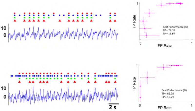
Detector Performance At Low SNR. The figure consists of two pre-processed intensity traces from the low SNR control (Top), and the low SNR isoproterenol (Bottom) drug treatments. The circles above each data trace represent the DEs identified by analysts 1–3 (bottom to top respectively). The triangles above each data trace represent MaD detected DEs, using the optimal thresholds identified in the corresponding ROC curves to the right. The error bars represent 95% confidence intervals. The optimal performance for each drug treatment case is presented under each ROC curve. As the SNR decreased, the performance of the MaD detector also decreased. Performance was still adequate for SNR ≃ 3, but not for SNR ≤ 1.

3.1.2. MaD Detector Performance

A total of 5 detection cases were considered: Control-1, Iso-1, Pro-1, Control-2, and Iso-2, where the last 2 (Control-2 and Iso-2) represent specially selected low-SNR data. Unanimous DEs between all 3 analysts were used as the ground-truth for assessing MaD performance. If a detected DE was within 0.12 s, or one quarter of the length of a typical DE, of the true peak time, it was considered a true positive (TP). Otherwise, the detected DE was considered a false positive (FP). Examples of detected DEs are shown in Figs. 2 and 3.

A true positive vector tp was used to represent all of the ground-truth DEs in a given detection case. If a given DE was successfully detected (TP) it was assigned a value of 1, and 0 otherwise. Similarly, a false positive vector fp was used to represent all of the detected DEs in a given detection case, with each detected DE assigned a value of 1 if the DE was a FP, and 0 otherwise. The means of tp and fp, representing TP and FP rates respectively, were then calculated at 45 incrementally increasing thresholds for each detection case. The TP and FP rates at each threshold were then used to generate receiver operating characteristic (ROC) curves for each detection case (Figs. 2 and 3).

The threshold at which detector performance is closest to TP = 100% and FP = 0% is the optimal threshold and constitutes the best detector performance for that detection case. All following performance metrics are presented as TP or FP Rate [95% confidence interval]. The best performance for the Control-1 case was TP = 97.92 [92.15, 100.00] % and FP = 1.75 [0.00, 5.26] % at a threshold of 4 standard deviations above the noise mean. The best performance for the Iso-1 case was TP = 100.00 [100.00, 100.00] % and FP = 0.78 [0.00, 2.33] % at a threshold of 8 standard deviations above the noise mean, and the best performance for the Pro-1 case was TP = 98.81 [96.43, 100.00] % and FP = 1.19 [0.00, 3.57] % at a threshold of 6 standard deviations above the noise mean. Overall, the MaD detector performed on par with human analysts and accurately identified DEs at SNR levels of 5 and above.

Performance decreased in the low-SNR detection cases. The best performance for the Control-2 case was TP = 72.37 [61.84, 81.58] % and FP = 16.67 [7.58, 25.76] % at a threshold of 4 standard deviations above the noise mean. The best performance for the Iso-2 case was TP = 65.79 [49.99, 81.59] % and FP = 13.79 [0.44, 27.14] % at a threshold of 2 standard deviations above the noise mean. Note that the training used for detection in the Control-2 and Iso-2 cases was derived from the Control-1 and Iso-1 data sets, respectively. The low analyst agreement, ranging from 76% to 69%, in these low-SNR detection cases made it very difficult to reliably select training samples from the Control-2 and Iso-2 data traces. Therefore, training from the higher SNR data traces had to be used instead. If training data could be reliably selected from the Control-2 and Iso-2 data traces, it is likely that the lower quality of the training samples would adversely affect detection performance.

3.1.3. White Gaussian Noise vs Fully Colored Noise

The full noise covariance extracted from the training data (Sec. 2.6.1) is a very accurate estimate of the noise parameters. However, if the training noise sample is too small the full noise covariance could be poorly estimated and it may be advantageous to make the simplifying assumption that the noise is temporally white. The parameters, Σ_i,j, of the noise covariance matrix Σ, are zero if i ≠ j, under the White Gaussian Noise (WGN) assumption. Furthermore, the diagonal parameters of Σ are all σ². The covariance matrix then takes on the form Σ = σ²I_N×N, and the matched filter output is then calculated as

$$S\left(x\right)=s\frac{1}{{\sigma }^2}{x}^T$$ (2)

We have tested the effects of employing the WGN assumption on the data presented in this paper. All subsequent results are presented at best performance as (TP%/FP%). Although the WGN assumption is a less accurate representation of the noise parameters than the full noise covariance, performance under the WGN assumption was not significantly affected in the Iso-1 (100.00%/0.78%) or Pro-1 (97.62%/2.38%) detection cases (ROC curves not shown in the interest of space). The Control-1 case, suffered slightly in performance (93.22%/5.17%), but is still within the previously quoted confidence interval. The Control-2 case showed a more marked decrease in detection efficacy (85.53%/32.29%). Curiously, the Iso-2 case, which has the lowest SNR of all of the data presented in this work, showed an increase in both the best TP rate, and the best FP rate (89.47%/34.62%), which resulted in a comparable overall performance.

These results imply that the matched filter under a WGN assumption is sufficient for DE detection at SNR levels of 5 and higher, but may lead to a decrease in detection efficacy at lower SNRs.

3.2. DE Analysis

The DEs detected at optimal thresholds as determined in Sec. 3.1.2 were used for spike analysis. All p-values associated with this analysis, as well as the average DEs of the treatments being compared, are shown in Figs. 4 and 5. Two DE groups were considered distinguishable if at least one of the metrics being measured (DE widths, upslopes and downslopes) were statistically different between the two groups, as determined by KS-tests. The drug treatments were first compared with controls, and then across time elapsed since drug administration.

Figure 4.

DE analysis with respect to drug treatment and time after drug administration. 6 panels are shown. Each panel shows the average DEs of the two specified drug treatments, with standard deviations shaded around the average. The title of each panel identifies the two treatments being compared. The text below the title indicates whether the DE populations were different in width, upslope, and downslope, and provides p-values. The top 3 panels, going from left to right, compare Iso-1 0min, (green) to Control-1 (red), Iso-1 10min (light teal) to Control-1, and Iso-1 0min to Iso-1 10min. Both Iso-1 0min and Iso-1 10min were different from Control-1, and were different from each other, in all three parameters (width, upslope, downslope). The bottom 3 panels, going from left to right, compare Pro-1 0min (purple) to Control-1 (red), the Pro-1 10min (blue) to Control-1, and Pro-1 0min to Pro-1 10min. Both Pro-1 0min and Pro-1 10min were different from Control-1 in width, upslope, and downslope. They were also different from each other in width, and upslope.

Figure 5.

DE analysis with respect to drug treatment for the lower SNR data. Iso-2 15min (orange) and Control-2 (red) were different in width, but not in upslope or downslope.

The higher SNR drug treated data (Iso-1 and Pro-1) were compared to the higher SNR control (Control-1). The Iso-1 0min drug treatment was statistically distinguishable from Control-1 in width (p-value = 3.6 × 10⁻⁵), upslope (p-value = 7.9 × 10⁻⁷), and downslope (p-value = 6.4 × 10⁻⁶). This difference was maintained 10 min after isoproterenol was administered (Iso-1 10min) (width p-value = 5.0 × 10⁻⁸, upslope p-value = 0.02, downslope p-value = 1.6 × 10⁻⁷). DEs measured immediately after propranolol administration (Pro-1 0min) were also already statistically distinguishable from Control-1 in width (p-value = 7.0 × 10⁻¹¹), upslope (p-value = 2.5 10⁻³), and downslope (p-value = 1.1 × 10⁻⁴). This difference was also maintained 10 min after propranolol was administered × (Pro-1 10min) (width p-value = 1.5 × 10⁻⁷, upslope p-value = 1.1 × 10⁻⁸, downslope p-value = 5.5 × 10⁻⁷). These results (shown in Fig. 4) indicate that this analysis method can distinguish DEs from control and drug treatments even less than a minute after the drug is administered (0min cases). The distinctions are also maintained 10 min after drug administration.

To show that the method is also applicable in a low-SNR setting, we performed a DE comparison analysis on Control-2 (average SNR = 3.07) and Iso-2 15min (average SNR = 0.63). The Iso-2 15min drug treatment was statistically distinguishable from Control-2 in width (p-value = 0.02), but not in either upslope (p-value = 0.68) or downslope (p-value = 0.25). These results are shown in Fig. 5. We would expect the DE width difference to be most pronounced among these two cases. This is reflected in the results. As SNR is decreased the DE widths remain the only distinguishable parameters, while upslope and downslope no longer differ between the two cases.

The drug treatments were then compared in time to evaluate if the 0 min cases could be distinguished from the 10 min cases. The Iso-1 0min case was statistically distinguishable from the Iso-1 10min case in all three parameters (width p-value = 2.2 × 10⁻⁴, upslope p-value = 1.6 × 10⁻⁵, downslope p-value = 8.3 × 10⁻⁴). The Pro-1 0min case was statistically distinguishable from the Pro-1 10min case in width (p-value = 0.01) and upslope (p-value = 1.4 × 10⁻³), but was not statistically different in downslope (p-value = 0.28).

In summary, KS-tests of DE widths, upslopes and downslopes revealed that DEs immediately after isoproterenol administration are distinguishable from controls. Similarly, DEs immediately after propranolol administration are distinguishable from controls. These differences are maintained 10 min after drug administration. DEs immediately after drug administration were also distinct from DEs 10 min after drug administration, in both the isoproterenol and propranolol cases. Lastly, isoproterenol treated cells were distinguishable from controls even at SNRs of 3 and below. These results indicate that KS-test comparisons of DE widths, upslopes, and downslopes, can accurately distinguish drug-treated DEs from controls, even at low SNRs, and can also distinguish drug-treated DEs based on the time after drug administration.

4. Discussion

4.1. Biological Relevance

Development of next generation human cardiac in vitro pre-clinical testing platforms is progressing at a rapid pace [4, 9, 20]. Non-invasive, high-throughput, automated electrophysiology analysis methods that can provide data at the subcellular scale in engineered 3D cardiac tissues are necessary to make these platforms feasible as a rapid and reliable predictor of the cardiac side effects of novel drugs under consideration for clinical trials. The combination of using image-based electrophysiology (2-photon microscopy of fluorescent VSD) and advanced automated signal processing (MaDEC) allows for the collection and quantitative analysis of electrophysiological data on the spatio-temporal scale needed in these advanced pre-clinical cardiac tissue models.

Furthermore, although the DEs presented here appear periodically, the MaD algorithm takes a generalized approach to signal detection. This allows for the detection of irregular DEs that may be indicative of drug-induced side effects. Early after depolarization (EAD) and delayed after depolarization (DAD) events are potentially lethal and may occur at irregular intervals [6, 28]. MaD does not incorporate the expected periodicity of cardiac DEs into the detection algorithm, allowing for the flexibility to detect these types of events. In the event that periodic signals are explicitly desired at low-SNR, the MaD detector could be modified to apply a variable threshold to pick up low-SNR DEs at the expected time intervals, without increasing the number of FPs throughout the entire dataset.

4.2. Effects of Differing Training Samples

For some applications, it may be advantageous to reduce the training samples size, in the interest of time. In our experience, the noise sample is highly dependent on the length of individual noise segments identified by the user. If long noise segments (more than 10 times the window size) are available, then as little as 10 segments can be sufficient for accurate DE detection. Similarly, the signal sample is dependent on SNR. If high SNR (SNR ≥ 5) DEs are available for training, then as little as 10 samples is sufficient for accurate DE detection. However, if the signal SNR is lower, then at least 20 samples should be used to maximize detection efficacy. Note that data pre-processing has little effect on SNR and serves only to remove large scale artifacts produced by the motion of the beating cell membrane and photobleaching of the VSD. Therefore variations in pre-processing methods should not affect the training paradigm.

It may also be useful to be able to re-use training samples between different data sets. To determine how re-using training samples from one data set to detect DEs from a different data set affects detection performance, we compared detection performance when a native training sample (derived from the data being tested) is used with detection performance when a non-native training sample (derived from data of a different cell membrane than the one being tested) is used. For this analysis we only tested the Control-1, Iso-1, and Pro-1 detection cases, as the low-SNR cases may not lead to reliable enough conclusions. All subsequent results are presented at best performance as (TP%/FP%). Using a non-native isoproterenol training sample on the Iso-1 data resulted in (96.88%/4.62%) using the full noise covariance, and (99.22%/0.78%) under the WGN assumption (ROC curves not shown in the interest of space). Similarly, using a non-native propranolol training sample on the Pro-1 data resulted in (90.48%/9.52%) using the full noise covariance, and (100.00%/0.00%) under the WGN assumption. In the Control-1 case, using a non-native control training sample resulted in (98.31%/1.69%) using the full noise covariance, and (96.61%/1.72%) under the WGN assumption. The detector worked well even when Iso-1 training was used on Pro-1 data (85.71%/26.53% using full noise covariance; 100.00%/0.00% under the WGN assumption) and vice versa (79.69%/28.67% using full noise covariance; 98.44%/1.56% under the WGN assumption).

In all of these cases we see that detection performance is maintained if a non-native training sample is used. Furthermore, efficacy is most often preserved under the WGN assumption. When the full noise covariance is used with a non-native training sample, detection performance may begin to degrade, indicating that in the absence of a native noise covariance, the filter may perform better using a WGN approximation than using a well estimated but inaccurate, non-native noise covariance.

4.3. DE Analysis

The automated MaDEC approach allows for quantitative comparison of DEs recorded from different drug treatments and time points using VSDs. In this study, MaDEC was able to identify significant changes in DE width, upslope, and downslope immediately after treatment with either propranolol or isoproterenol. These changes were sustained when measured 10 min after exposure to each drug. Furthermore, MaDEC identified changes in DE width between isoproterenol treated cells and controls, even at SNRs of 3 and below. Propranolol and isoproterenol both act on β-adrenoreceptors in cardiac cells as a β-blocker and β-adrenergic agonist, respectively. β-adrenoreceptors modulate calcium influx during an action potential.

Calcium transport from the L-type calcium channels determines the delay before repolarization. This delay determines the width of the DE, also known as the plateau phase. The upslope of a cardiac action potential, primarily driven by fast sodium channels, would not be expected to be affected by β-adrenergic modulation [17]. The downslope may be affected to a lesser degree than the width since the balance of decreasing calcium channel activity and increasing delayed rectifier potassium channel (I_KS, I_KR, I_K1) activity initiate the downslope.

Both isoproterenol- and propranolol-treated cell behavior, quantified by MaDEC, exhibited significant changes in width and downslope after drug administration. However, the cells also demonstrated an unexpected difference in upslope after drug administration. For the isoproterenol-treated cells, this difference decreased with time (p-value = 7.9 × 10⁻⁷ for Iso-1 0min vs Control-1, and p-value = 0.02 for Iso-1 10min vs Control-1), and seemed to be trending towards being insignificant. This indicates that the difference in upslope may be due to an initial shock from isoproterenol administration and that the effects may fade as the tissue stabilizes. In contrast, the difference in upslope seemed to increase in time for the propranolol-treated cells (p-value = 2.5 × 10⁻³ for Pro-1 0min vs Control-1, and p-value = 1.1 × 10⁻⁸ for Pro-1 10min vs Control-1). However, both of the p-values are so close to zero, that they’re difficult to reliably compare. When low-SNR isoproterenol-treated cell data (Iso-2 15min) was compared with a low-SNR control (Control-2), only differences in DE widths were detected. Finally, we’d like to note that the DE widths of isoproterenol-treated cells increased with respect to controls, in both low-SNR and high-SNR scenarios. The mechanism of action of isoproterenol (β-adrenergic agonists) would lead us to expect a decrease in the width of the DE. Despite this unexpected, yet consistent, result, MaDEC still correctly identified and quantified the effect of the drug, emphasizing its impartial approach to DE detection and analysis.

4.4. Comparison with Existing Methods

VSDs address limitations of existing methods for measuring hiPS-CM DEs. Patch clamping offers precise measurement of transmembrane voltages, but is invasive in nature, requiring destructive membrane puncture to position electrodes that prevents longitudinal experiments. Only single cells may be assessed using a complex apparatus [2, 13, 26]. The growing field of organ-on-a-chip platforms demands non-invasive fluorescence based in situ endpoints for assessing hiPS-CM [12, 19]. VSD fluorescence intensity measurements using 2-photon microscopy are noninvasive, non-destructive, and allow for longitudinal electrophysiological assessment of live, 3D, cardiac tissues in microfluidic-based devices.

Quantitative assessment of the heterogeneity of the DEs of actively beating cardiomyocytes is critical to understanding the electrophysiology underlying these cardiac tissue models. Many existing quantitative analysis tools studying cardiomyocyte activity were developed for calcium imaging applications. These are often focused on automated region of interest (ROI) identifications [22, 3, 1]. These image analysis tools are not readily applicable to VSD imaging of cell membranes, where two-dimensional regions of interest, are not necessarily spherical and are more difficult to identify. Algorithms focusing on line-scan data, and similar to the MaD detector presented here, have been developed for Ca²⁺ spark detection in cardiac ventricular myocytes [14], as well as elementary calcium release events in muscle [27]. However, these algorithms focus only on detecting the signal and do not provide further analysis tools for quantitatively assessing changes in tissue or cell activity with varying experimental parameters (such as drug administration). MaDEC can automatically and accurately detect, extract, quantify, and compare VSD-based DEs across drug treatments and time points after drug administration. Unlike other VSD-approaches that use pre-defined waveform features, MaDEC uses a data-driven sample of the entire waveform to detect DEs, resulting in a non-biased DE selection criterion that can accurately detect waveforms at SNRs ≥ 3. Also, unlike other approaches, DE parameters such as width, upslope and downslope, are compared across normalized waveform populations. The method’s lack of reliance on absolute fluorescence amplitude ensures that results are not biased by the amount of dye the cells took up, or the cells’ exact positions in the imaging plane.

5. Conclusion

MaDEC is a useful new tool for the study of cardiomyocyte electrophysiology. Combined with the use of voltage-sensitive dyes, it allows for non-invasive, image-based, and automated analysis of cardiac DEs. This study demonstrates the ability of this tool to detect and quantify changes in DEs as a function of drug treatment and as a function of time. The software is freely available at sites.uci.edu/aggies/downloads or from the corresponding author, and can be easily modified to assess the electrophysiology of other excitable cell populations (e.g. neurons) [23] and data types (e.g. calcium reporters, patch clamp) [24].

Supplementary Material

1

Figure 6: Motion Artifact Correction. Motion artifact resulting from the spontaneous beating of cell clusters was compensated for in data pre-processing using a Gaussian tracking and correction algorithm. Quantification of membrane 3 depolarization peaks using pre-corrected raw data correlates well with membrane 1 depolarization peaks quantified using data corrected with the Gaussian tracking algorithm.

2

Figure 7: Photobleaching Correction. Photobleaching was accounted for by fitting a biexponential (y = ae^bx + ce^dx) and subtracting from the signal. (Top) Raw signal collected by the instrument. (Middle) Overlay of second order exponential fit and raw signal. (Bottom) Resultant signal after subtracting the exponential fit and normalizing to baseline fuorescence of the membrane (F_o).

References

- 1.Bányász T, Chen-Izu Y, Balke CW, Izu LT. A new approach to the detection and statistical classification of Ca2+ sparks. Biophysical Journal. 2007;92(12):4458–4465. doi: 10.1529/biophysj.106.103069. [DOI] [PMC free article] [PubMed] [Google Scholar]
- 2.Bébarová M. Advances in patch clamp technique: towards higher quality and quantity. General Physiology and Biophysics, pages. 2012:131–140. doi: 10.4149/gpb_2012_016. [DOI] [PubMed] [Google Scholar]
- 3.Bray MA, Geisse NA, Parker KK. Multidimensional detection and analysis of Ca2+ sparks in cardiac myocytes. Biophysical Journal. 2007;92(12):4433–4443. doi: 10.1529/biophysj.106.089359. [DOI] [PMC free article] [PubMed] [Google Scholar]
- 4.Devalla HD, Schwach V, Ford JW, Milnes JT, El-haou S, Jackson C, Gkatzis K, Elliott DA, Chuva SM, Lopes DS, Mummery CL, Verkerk AO, Passier R. Atrial-like cardiomyocytes from human pluripotent stem cells are a robust preclinical model for assessing atrial-selective pharmacology. EMBO Molecular Medicine. 2015;7(4):394–410. doi: 10.15252/emmm.201404757. [DOI] [PMC free article] [PubMed] [Google Scholar]
- 5.Ellefsen KL, Settle B, Parker I, Smith IF. An algorithm for automated detection, localization and measurement of local calcium signals from camera-based imaging. Cell Calcium. 2014;56(3):147–156. doi: 10.1016/j.ceca.2014.06.003. [DOI] [PMC free article] [PubMed] [Google Scholar]
- 6.Gaztañaga L, Marchlinski FE, Betensky BP. Mechanisms of Cardiac Arrhythmias. Revista Española de Cardiología (English Edition) 2012;65(2):174–185. doi: 10.1016/j.recesp.2011.09.018. [DOI] [PubMed] [Google Scholar]
- 7.Ghouri IA, Kelly A, Burton FL, Smith GL, Kemi OJ. 2-photon excitation fluorescence microscopy enables deeper high-resolution imaging of voltage and Ca2+ in intact mice, rat, and rabbit hearts. Journal of Biophotonics. 2013;123(1):112–123. doi: 10.1002/jbio.201300109. [DOI] [PubMed] [Google Scholar]
- 8.Goldsmith CJ, Städele C, Stein W. Optical imaging of neuronal activity and visualization of fine neural structures in non-desheathed nervous systems. PloS ONE. 2014;9(7) doi: 10.1371/journal.pone.0103459. [DOI] [PMC free article] [PubMed] [Google Scholar]
- 9.Harris K, Aylott M, Cui Y, Louttit JB, McMahon NC, Sridhar A. Comparison of electrophysiological data from human-induced pluripotent stem cell-derived cardiomyocytes to functional preclinical safety assays. Toxicological Sciences. 2013;134(2):412–426. doi: 10.1093/toxsci/kft113. [DOI] [PubMed] [Google Scholar]
- 10.Herron T, Lee P, Jalife J. Optical imaging of voltage and calcium in cardiac cells & tissues. Circulation Research. 2012;110(4):609–623. doi: 10.1161/CIRCRESAHA.111.247494. [DOI] [PMC free article] [PubMed] [Google Scholar]
- 11.Heylman CM, Datta R, Sobrino A, George S, Gratton E. Supervised Machine Learning for Classification of the Electrophysiological Effects of Chronotropic Drugs on Human Induced Pluripotent Stem Cell-Derived Cardiomyocytes. PLoS ONE. 2015;12(10) doi: 10.1371/journal.pone.0144572. [DOI] [PMC free article] [PubMed] [Google Scholar]
- 12.Heylman CM, Santoso S, Krebs MD, Saidel GM, Alsberg E, Muschler GF. Modeling and experimental methods to predict oxygen distribution in bone defects following cell transplantation. Medical & Biological Engineering & Computing. 2014;52(4):321–30. doi: 10.1007/s11517-013-1133-7. [DOI] [PubMed] [Google Scholar]
- 13.Huang D, Li J. The feasibility and limitation of patch-clamp recordings from neonatal rat cardiac ventricular slices. In Vitro Cellular and Developmental Biology - Animal. 2011;47:269–272. doi: 10.1007/s11626-011-9387-6. [DOI] [PubMed] [Google Scholar]
- 14.Kong CHT, Soeller C, Cannell MB. Increasing sensitivity of Ca2+ spark detection in noisy images by application of a matched-filter object detection algorithm. Biophysical Journal. 2008;95(12):6016–6024. doi: 10.1529/biophysj.108.135251. [DOI] [PMC free article] [PubMed] [Google Scholar]
- 15.Leyton-Mange JS, Mills RW, Macri VS, Jang MY, Butte FN, Ellinor PT, Milan DJ. Rapid cellular phenotyping of human pluripotent stem cell-derived cardiomyocytes using a genetically encoded fluorescent voltage sensor. Stem Cell Reports. 2014;2(2):163–70. doi: 10.1016/j.stemcr.2014.01.003. [DOI] [PMC free article] [PubMed] [Google Scholar]
- 16.Lian X, Zhang J, Azarin SM, Zhu K, Hazeltine LB, Bao X, Hsiao C, Kamp TJ, Palecek SP. Directed cardiomyocyte differentiation from human pluripotent stem cells by modulating Wnt/β-catenin signaling under fully defined conditions. Nature Protocols. 2013;8(1):162–75. doi: 10.1038/nprot.2012.150. [DOI] [PMC free article] [PubMed] [Google Scholar]
- 17.Ma J, Guo L, Fiene SJ, Anson BD, Thomson JA, Kamp TJ, Kolaja KL, Swanson BJ, January CT. High purity human-induced pluripotent stem cell-derived cardiomyocytes: electrophysiological properties of action potentials and ionic currents. AJP: Heart and Circulatory Physiology. 2011;301(5):H2006–H2017. doi: 10.1152/ajpheart.00694.2011. [DOI] [PMC free article] [PubMed] [Google Scholar]
- 18.Mordwinkin N, Burridge P, Wu J. A review of human pluripotent stem cell-derived cardiomyocytes for high-throughput drug discovery, cardiotoxicity screening and publication standards. Journal of Cardiovascular Translational Research. 2013;6(1):22–30. doi: 10.1007/s12265-012-9423-2. [DOI] [PMC free article] [PubMed] [Google Scholar]
- 19.Moya M, Tran D, George SC. An integrated in vitro model of perfused tumor and cardiac tissue. Stem Cell Research & Therapy. 2013;4(Suppl 1(Suppl 1)):S15. doi: 10.1186/scrt376. [DOI] [PMC free article] [PubMed] [Google Scholar]
- 20.Schaaf S, Shibamiya A, Mewe M, Eder A, Stöhr A, Hirt MN, Rau T, Zimmermann WH, Conradi L, Eschenhagen T, Hansen A. Human engineered heart tissue as a versatile tool in basic research and preclinical toxicology. PLoS ONE. 2011;6(10) doi: 10.1371/journal.pone.0026397. [DOI] [PMC free article] [PubMed] [Google Scholar]
- 21.Senseman DM. Correspondence between visually evoked voltage-sensitive dye signals and synaptic activity recorded in cortical pyramidal cells with intracellular microelectrodes. Visual Neuroscience. 1996;13(5):963–77. doi: 10.1017/s0952523800009196. [DOI] [PubMed] [Google Scholar]
- 22.Steele EM, Steele DS. Automated detection and analysis of Ca2+ sparks in x-y image stacks using a thresholding algorithm implemented within the open-source image analysis platform ImageJ. Biophysical Journal. 2014;106(3):566–576. doi: 10.1016/j.bpj.2013.12.040. [DOI] [PMC free article] [PubMed] [Google Scholar]
- 23.Szymanska A, Doty M, Scannell KV, Nenadic Z. A supervised multi-sensor matched filter for the detection of extracellular action potentials. Proc of the 36th Annual International Conference of the IEEE Engineering in Medicine and Biology Society. 2014:5996–9. doi: 10.1109/EMBC.2014.6944995. [DOI] [PubMed] [Google Scholar]
- 24.Szymanska AF, Kobayashi C, Norimoto H, Ikegaya Y, Nenadic Z. Accurate detection of low signal-to-noise ratio neuronal calcium transient waves using a matched filter. Journal of Nueroscience Methods. 2016;259:1–12. doi: 10.1016/j.jneumeth.2015.10.014. [DOI] [PubMed] [Google Scholar]
- 25.Vallmitjana A, Barriga M, Nenadic Z, Llach A, Alvarez-Lacalle E, Hove-Madsen L, Benitez R. Identification of intracellular calcium dynamics in stimulated cardiomyocytes. Proc of the 32th Annual International Conference of the IEEE Engineering in Medicine and Biology Society. 2010:68–71. doi: 10.1109/IEMBS.2010.5626238. [DOI] [PubMed] [Google Scholar]
- 26.Wang L, Chen T, Zhou X, Huang Q, Jin C. Atomic force microscopy observation of lipopolysaccharide-induced cardiomyocyte cytoskeleton reorganization. Micron. 2013;51:48–53. doi: 10.1016/j.micron.2013.06.008. [DOI] [PubMed] [Google Scholar]
- 27.Wegner Fv, Both M, Fink RHA. Automated detection of elementary calcium release events using the á trous wavelet transform. Biophysical Journal. 2006;90(6):2151–2163. doi: 10.1529/biophysj.105.069930. [DOI] [PMC free article] [PubMed] [Google Scholar]
- 28.Weiss JN, Garfinkel A, Karagueuzian HS, Chen PS, Qu Z. Early afterdepolarizations and cardiac arrhythmias. Heart Rhythm. 2010;7(12):1891–1899. doi: 10.1016/j.hrthm.2010.09.017. [DOI] [PMC free article] [PubMed] [Google Scholar]
- 29.Yan P, Acker CD, Zhou WL, Lee P, Bollensdorff C, Negrean A, Lotti J, Sacconi L, Antic SD, Kohl P, Mansvelder HD, Pavone FS, Loew LM. Palette of fluorinated voltage-sensitive hemicyanine dyes. Proceedings of the National Academy of Sciences of the United States of America. 2012;109(50):20443–8. doi: 10.1073/pnas.1214850109. [DOI] [PMC free article] [PubMed] [Google Scholar]
- 30.Zeevi-Levin N, Itskovitz-Eldor J, Binah O. Cardiomyocytes derived from human pluripotent stem cells for drug screening. Pharmacology & Therapeutics. 2012;134(2):180–8. doi: 10.1016/j.pharmthera.2012.01.005. [DOI] [PubMed] [Google Scholar]
Associated Data
This section collects any data citations, data availability statements, or supplementary materials included in this article.
Supplementary Materials