Quabantitative interpretation of molecular dynamics simulations for X-ray photoelectron spectroscopy of aqueous solutions

Abstract

Over the past decade, energy-dependent ambient pressure X-ray photoelectron spectroscopy (AP-XPS) has emerged as a powerful analytical probe of the ion spatial distributions at the vapor (vacuum)-aqueous electrolyte interface. These experiments are often paired with complementary molecular dynamics (MD) simulations in an attempt at to provide a complete description of the liquid interface. There is, however, no systematic protocol that permits a straightforward comparison of the two sets of results. XPS is an integrated technique that averages signals from multiple layers in a solution even at the lowest photoelectron kinetic energies routinely employed, whereas MD simulations provide a microscopic layer-by-layer description of the solution composition near the interface. Here we use the National Institute of Standards and Technology database for the Simulation of Electron Spectra for Surface Analysis (SESSA) to quantitatively interpret atom-density profiles from MD simulations for XPS signal intensities using sodium and potassium iodide solutions as examples. We show that electron inelastic mean free paths calculated from a semi-empirical formula depend strongly on solution composition, varying by up to 30 % between pure water and concentrated NaI. The XPS signal thus arises from different information depths in different solutions for a fixed photoelectron kinetic energy. XPS signal intensities are calculated using SESSA as a function of photoelectron kinetic energy (probe depth) and compared with a widely employed ad hoc method. SESSA simulations illustrate the importance of accounting for elastic scattering events at low photoelectron kinetic energies (< 300 eV) where the ad hoc method systematically underestimates the preferential enhancement of anions over cations. Finally, some technical aspects of applying SESSA to liquid interfaces are discussed.

I. Introduction

Core-level X-ray photoelectron spectroscopy (XPS) is a chemical-specific analytical technique that many consider to be the workhorse of surface and interface science. Major advantages of XPS are its surface sensitivity,¹ its ability to detect every element of the periodic table except hydrogen, and the fact that many compounds can be analyzed without significant decomposition by the incident X-ray beam. In order, however, to interpret XPS signal intensities quantitatively, a comprehensive understanding of the attenuation and scattering of the photoelectrons in the sample is required. One important sample parameter in this regard is the electron inelastic mean free path (IMFP), which together with the photoelectron emission angle determines in large part the surface sensitivity of XPS experiments.¹ In solids, appropriate models and the required data are available for accurate predictions of IMFPs for energies greater than 50 eV,^2–4 many of which have been confirmed experimentally.⁵ In liquids, more specifically in aqueous solutions, consensus remains elusive and several publications report substantially different values for the electron IMFP.^6–10 This poor understanding of the electron IMFP limits the ability to quantitatively interpret XPS signal intensities from aqueous solutions.

In order to quantitatively describe the structure of an aqueous solution interface, it is commonplace to turn to molecular dynamics (MD) simulations for confirmation of depth-resolved, a term that is interchangeable with energy-dependent, XPS signal intensities.^{7, 11–14} MD simulations yield molecular-level solute (typically an electrolyte) and solvent (most often water) distributions with respect to depth and, over the past decade, have contributed enormously to our microscopic understanding of the vapor (or vacuum)-aqueous electrolyte interface.¹⁵ Direct comparison of MD simulations with XPS signal intensities are, however, not straightforward. MD simulations provide an atomic-scale description of molecular distributions in the vicinity of the interface, whereas XPS is an integrated technique that samples a depth that depends on the IMFP for the photoelectron energy, the photoelectron emission angle, and a parameter describing the strength of elastic scattering.¹ The crux of the problem is, therefore, to relate water and solute distributions obtained from MD simulations to the XPS signal intensities measured for different photoelectron energies. The solution requires better knowledge of the IMFP as a function of energy for water and aqueous solutions. In this article we describe what we believe to be the first quantitative interpretation of MD simulation profiles for XPS signal intensities of aqueous solutions of 2 mol/L KI and 1 mol/L NaI.

The present contribution is not intended to entirely resolve the debate surrounding the energy dependence of the probe depth in XPS experiments on aqueous solutions (the resolution will most likely come from novel experiments), but rather sets out to establish straightforward and consistent protocol using the National Institute of Standards and Technology (NIST) database for the Simulation of Electron Spectra for Surface Analysis (SESSA)^16,17 to enable a direct interpretation of MD simulations with XPS signal intensities. As our understanding of electron IMFPs and elastic-scattering effects in aqueous solutions continues to evolve, the calculations reported herein can be updated.

II. Methods

A. Molecular Dynamics Simulations

MD simulations of ≈2 mol/L KI (68 ions and 1728 water molecules) and ≈1 mol/L NaI (32 ions and 1728 water molecules) solutions were performed using the Gromacs simulation suite,^18–22 version 4.6.3. The ions and water molecules were placed in a simulation cell of dimensions 3 nm × 3 nm × 14 nm in the x, y, and z directions, respectively. The simulations were carried out with three-dimensional periodic boundary conditions and a timestep of 2 fs for 100 μs (excluding equilibration time); two interfaces formed spontaneously during the equilibration. The average temperature was held at 300 K using a Berendsen thermostat with an additional stochastic term that ensures the correct kinetic energy distribution.²³ The non-polarizable force field developed by Horinek et al²⁴ was used to model the ions, and the Simple Point Charge/Extended (SPC/E) model was used for the water molecules.²⁵ The Lennard-Jones parameters σ and ɛ, and charges associated with each atom type are listed in Table 1. Electrostatic interactions were calculated using the smooth particle-mesh-Ewald method,²⁶ and a cutoff of 0.9 nm was used for the Lennard-Jones interactions and the real-space part of the Ewald sum. Water molecules were held rigid by using the SETTLE algorithm.²⁷ The average bulk concentrations are computed from the compositions of the innermost 2 nm of the simulated slabs: 0.96 mol/L for NaI and 2.07 mol/L for KI.

TABLE 1.

Molecular dynamics (MD) simulation parameters

Ion	Charge	σ(nm)24	ɛ (kJ/mol)24	ξ(nm)	η
O	−0.8476	0.3166	0.65	0.24	1.0
H	+0.4238	–	–	–	–
Na+	+1	0.2234	0.65	–	–
K+	+1	0.2945	0.65	–	–
I−	−1	0.5014	0.9846	0.27	3.35

The ion force fields used here were optimized in conjunction with SPC/E water to reproduce ion solvation free energies and entropies, as well as the positions of the first peaks in the ion-water radial distribution functions.²⁴ The resulting models were used to calculate potentials of mean force for the adsorption of single ions to the vapor/water interface, which served as input to extended Poisson-Boltzmann calculations of ion concentration profiles.²⁴ The latter were used to calculate surface tension increment (difference between the surface tension of a salt solution and the surface tension of neat water). The surface tension increments obtained from the parameter set employed herein agreed well with experimental data up to 1 mol/L.²⁴ The surface tension increments calculated from our simulations, 0.79 mN/m for 0.96 mol/L NaI and 1.55 mN/m for 2.07 mol/L KI, are in reasonable agreement with the experimental values of 1.01 mN/m for 1.0 mol/L NaI and 1.92 mN/m for 2.0 mol/L KI at 293 K.²⁸ In addition, the bulk solution densities calculated from our simulations, 1085 kg/m³ for 0.96 mol/L NaI and 1263 kg/m³ for 2.07 mol/L KI, agree very well with the experimental values of 1106 kg/m³ and 1246 kg/m³, respectively, interpolated from tabulated measurements at 298 K.²⁹

B. Interface Definitions

Due to thermal fluctuations, the surface boundary separating the liquid and vapor phases is a dynamic and rough interface that evolves along with the movement of the molecules in solution. A common definition of the location of the interface is the Gibbs dividing surface (GDS). In MD simulations, the GDS is located first by computing the water O atom density profile in a static coordinate system, which averages over the the thermal fluctuations. The GDS is the position along the coordinate (z) normal to the interface at which the solvent density is equal to half its bulk value. In this study, we implement an additional definition of the interface, the so-called “instantaneous interface”, proposed by Willard and Chandler.³⁰ The use of the instantaneous interface as the origin of the interfacial coordinate yields density profiles with molecular-scale resolution. To locate the instantaneous interface, the nuclear positions of each water molecule and ion are convoluted with three-dimensional Gaussian density distribution’s, with standard deviations ξ and magnitudes η listed in Table 1, to construct a density field over the entire simulation cell. The instantaneous interfaces are then determined at each time step as the locus of points at which the density field is equal to half the bulk solution density. To compute the density profiles, the positions of each water molecule and ion are then referenced to the nearest instantaneous interface (above or below). Further details on the implementation of the instantaneous interface for interfaces of vapor (vacuum) and water or aqueous salt solutions are available in the literature.^30,31 In light of the fact that the escape of photoelectrons from solution at the kinetic energies and information depths of relevance in this study is extremely fast (≈0.5 × 10⁻¹⁵ second) compared to the thermal fluctuations of the interface (≈10 × 10⁻¹² second³⁰), the instantaneous interface representation is considered more appropriate than the GDS for comparing MD simulations with XPS data.

C. Simulation of Electron Spectra for Surface Analysis (SESSA)

XPS signal intensities are simulated using the SESSA software developed by Werner et al^16,17 SESSA is a NIST standard reference database that contains all data needed for quantitative simulations of XPS and Auger-electron spectra. Data retrieval is based on an expert system that queries the databases for each needed parameter. SESSA performs simulations of photoelectron intensities for user-specified conditions such as the morphology of the sample, the composition and thickness of each layer of a film or the composition and dimensions of a nanostructure, the X-ray source and its polarization, and the experimental configuration. SESSA provides the spectral shape of each photoelectron peak using a model of signal generation in XPS that includes multiple inelastic and elastic scattering of the photoelectrons. In order to minimize the computation time, an efficient Monte Carlo code is employed based on the trajectory-reversal method¹⁴ In contrast to conventional Monte Carlo codes where electrons are tracked based on their trajectories from the source to the detector, the trajectory-reversal approach tracks electrons in the opposite direction, starting from the detector and working back to the point of origin. Thus, all electrons contribute to the signal, which results in significantly decreased simulation times.

For the SESSA simulations reported in this article, the orientation of the analyzer axis is perpendicular to the X-ray source, while the sample surface normal is oriented in the same direction as the analyzer axis. The excitation source is a linearly polarized X-ray beam. The polarization vector is rotated 54.7° from the analyzer detection axis, which corresponds to the so-called magic angle in which the XPS intensity is independent of the emission angle. The acceptance solid angle for the detector is ±11° and the illuminated area on the sample is independent of the emission angle. The last condition is valid when the X-rays are focused in a relatively small area, as is the case for synchrotron or monochromatic laboratory sources. Our calculations employ electron IMFPs calculated via the semi-empirical TPP-2M formula of Tanuma et al.³ integrated within SESSA. The calculated IMFPs, which depend on the material density (ρ), atomic or molecular mass, number of valence electrons per atom or molecule, and the band-gap energy, are expected to have uncertainties of about 10 %, although the uncertainty could be larger for a small number of materials.³² XPS spectra are simulated for two orbitals of each of the elements present in the solutions (O 1s and O 2s; K 2p and 3p; I 4d and I 3d; Na 2p and Na 2s) using different x-ray wavelengths such that the photoelectron energies of particular lines of interest have the same kinetic energies. This procedure is employed so that the IMFPs of the photoelectrons for the different components within a given solution are the same. The photoelectron energy is varied between 65 eV, where a pronounced minimum in the probing depth of dilute aqueous solution has been proposed³³ and 1500 eV. The latter energy corresponds roughly with the energy of a laboratory X-ray Al K-α source (1487eV) and with what is available from most soft X-ray synchrotron beamlines with useful flux. A total of 26 photoelectron energies were simulated. The simulated intensities are then normalized by the atomic photoionization cross sections (available in SESSA) of Yeh and Lindau.³⁴

III. Results and Discussion

A. The Information Depth of XPS

The information depth (ID) or sampling depth is a measure of the surface sensitivity in a particular XPS experiment and is defined as the maximum depth, normal to the specimen surface, from which useful signal information is obtained.³⁵ Jablonski and Powell developed the following empirical equation for the ID, S:³⁶

$$S=\lambda \cos \alpha (1-0.787\omega )\text{ln}\left[\frac{1}{1-(P/100)}\right]$$ (1)

where λ is the IMFP, α is the photoelectron emission angle with respect to the surface normal, P is a specified percentage of the detected signal, and ω is a convenient measure of the strength of elastic-scattering effects on the photoelectron trajectories.^1,37 The ω parameter has a complicated dependence on electron energy and material^{1, 2} but is typically small (<0.1) for low atomic numbers (Z < 13) at an energy of 1500 eV but can be larger (≈ 0.4) at much lower energies (e.g., 65 eV). We note that Eq. 1 was derived for a homogeneous sample and is normally used for estimating IDs for the detection of most of the photoelectron signal of interest. Values of P = 90%, P = 95 %, or P = 99 % are typically used.

The majority of XPS experiments from aqueous solutions are performed at soft X-ray synchrotron beamlines where the energy range of practical interest varies from roughly 65 eV to 1500 eV.^{6–8, 10–14} The ID for a semi-infinite, structureless slab (a bulk liquid with no structure at the interface) of pure liquid water was calculated from Eq. (1) and is shown in Figure 1 for an emission angle α = 0°. The ω parameter was obtained from IMFP values at 65 eV (0.77 nm) and 1500 eV (5.03 nm) that were calculated from the predictive TPP-2M equation³ and from values of the transport mean free path (TMFP) that were retrieved from the SESSA database (1.07 nm and 92.74 nm for energies, E, of 65 eV and 1500 eV, respectively). These IMFP and TMFP values result in ω = 0.418 at 65 eV and ω = 0.052 at 1500 eV, with the larger ω highlighting the importance of elastic-scattering at lower energies. As expected, the surface sensitivity is significantly higher at 65 eV than it is at 1500 eV.

FIG. 1.

Plot of the information depth for liquid water from Eq. 1 as a function of the percentage, P, of the detected XPS signal for photoelectron energies, E, of 65 eV (red solid line) and 1500 eV (blue dashed line).

The contribution of the outermost molecular layer of water (0.3 nm) to the overall photoelectron signal can be determined from Figure 1. We find this layer contributes only 6 % at an energy of 1500 eV (S = 14.5 nm for P = 95 %) but 44 % at 65 eV(S = 1.5 nm for P = 95 %). The former value reveals the lack of surface/interface sensitivity when working at 1500 eV in aqueous solution, whereas the latter value demonstrates the inability of XPS to probe exclusively the outermost molecular layer of solution for normal emission of the photoelectrons (α = 0°). Analogous contributions can be determined for the outermost 1.5 nm of solution (the thickness of the interface region for 2 mol/L KI from the MD simulations, see Section III C). At 1500 eV, the outermost 1.5 nm of solution contributes 27 % to the overall signal intensity, whereas at 65 eV virtually all the signal (96 %) originates from this region and almost none of the bulk solution is sampled.

B. Relation Between Electron Kinetic Energy and Electron IMFP

Photoelectron experiments using X-rays from a synchrotron source are attractive in that the surface sensitivity can be varied simply by changing the X-ray wavelength so that the energy of a particular photoelectron peak corresponds to a desired value of the IMFP for a given material.^{38, 39}

The energy-dependent IMFPs from the TPP-2M equation³ for semi-infinite structureless slabs of water (blue circles), and 1 mol/L (green diamonds) and 10 mol/L (red squares)aqueous solutions of NaI are shown in Figure 2 and tabulated in Table 2. The command line inputs in SESSA for composition and density are /H2/O/ and ρ = 9.90 × 10²² atoms/cm³ for wate, (/H2/O/)98.78(/Na/)0.61(/I/)0.61 and ρ = 9.42 × 10²² atoms/cm³ for 1 mol/L NaI, and (/H2/O/)81.65(/Na/)9.17(/I/)9.17 and ρ = 6.54 × 10²² atoms/cm³ for 10 mol/L NaI, and the band-gap energy (E_g) is assumed constant (7.9 eV) for all three solutions (further discussion on E_g is given in Section III G). The numbers after each species specify the fractional contribution of each atom to the total atom density of the solution. The electron IMFP monotonically increases in all cases from a minimum at an energy of 65 eV to a maximum at 1500 eV. The calculated electron IMFPs become systematically lower over the entire energy range going from pure water to 1 mol/L and finally 10 mol/L NaI. This result makes clear that a universal curve of electron IMFP as a function of energy likely does not exist for aqueous solutions and, therefore, electron IMFPs will have to be calculated (or determined experimentally) for a wide range of solution compositions.

FIG.2.

Dependence of the electron IMFP on photoelectron kinetic energy. IMFPs for bulk solutions of neat water (blue circles), 1 mol/L (green diamonds) and 10 mol/L NaI (red squares) were calculated with the TPP-2M formula³ in SESSA. The simulated systems comprise semi-infinite structureless slabs.

TABLE 2.

Electron IMFPs from the TPP-2M equation³ for water, 1 mol/L NaI, and 10 mol/L NaI for electron energies from 65 eV to 1500 eV.

Energy (eV)	IMFP (nm) Water	IMFP (nm) 1 mol/L NaI	IMFP (nm) 10 mol/L NaI
65	0.77	0.72	0.58
70	0.78	0.73	0.60
80	0.81	0.76	0.62
90	0.83	0.78	0.65
100	0.86	0.81	0.67
110	0.89	0.84	0.70
120	0.92	0.87	0.73
130	0.95	0.90	0.76
140	0.98	0.93	0.79
150	1.01	0.96	0.81
160	1.05	0.99	0.84
170	1.08	1.03	0.87
180	1.11	1.06	0.90
190	1.14	1.09	0.93
200	1.18	1.12	0.96
250	1.34	1.28	1.10
300	1.51	1.44	1.24
400	1.83	1.76	1.50
500	2.15	2.06	1.71
600	2.46	2.36	2.02
700	2.76	2.65	2.27
800	3.06	2.93	2.51
900	3.35	3.21	2.75
1000	3.64	3.49	2.98
1250	4.35	4.17	3.55
1500	5.03	4.82	4.11

C. Molecular Dynamics Simulations

Ion populations in the vicinity of a solution/vapor interface are often different from the bulk solution composition, and their distributions are typically depicted as density profiles. Here we consider a MD simulation of a 2 mol/L KI solution, a snapshot from which is shown in Figure 3a. Density profiles have been calculated in the GDS and in the instantaneous-interface representations. Figure 3b plots the number density of water (blue), I⁻ (green) and K⁺ (red) as functions of the distance to the GDS, which is the location along z where the mean water density is equal to half its bulk value. Figure 3c plots the same quantities as a function of the distance to the instantaneous interface, which varies from one configuration to another. In both Figure 3b and Figure 3c, the density profiles have been positioned such that the interface is at z = 0 nm. Negative values of the horizontal axis indicate depth into the solution.

FIG. 3.

Molecular dynamics (MD) simulation results. a) Snapshot (side view) of an equilibrated simulation of 2 mol/L KI. The solution/vapor interface is at the upper end of the image. Red: potassium cations. Green: iodide anions. Blue/white: water molecules. b) Atomic density profiles using the Gibbs dividing surface (GDS) definition of the interface. c) Same as in b) except with the instantaneous definition of the interface. Note that both b) and c) are derived from the same simulation of the system shown in a).

In both the GDS and instantaneous-interface representations, we observe an enhancement in the ion populations in the vicinity of the interface relative to the bulk. In the GDS representation (Figure 3b), the density of iodide is enhanced (with respect to the bulk density) with a maximum occurring approximately −0.25 nm from the interface. An enhancement in the potassium density is observed in the “depletion layer” of the iodide profile, with a maximum number density at approximately −0.7 nm. The densities of both potassium and iodide ions converge to bulk values at about −1.2 nm. In the water density profile, bulk behavior is observed until approximately −0.2 nm, above which it decreases monotonically to zero.

In the instantaneous interface representation (Figure 3c), a clear structuring in the water and ion density profiles is observed near the interface. The water density exhibits two pronounced layers with density maxima at −0.1 nm and −0.6 nm from the interface, respectively. A significant enhancement in the iodide density occurs just behind the first water-peak, at −0.15 nm. Potassium density fills the depletion layer following the iodide enhancement, with the enhancement spanning the region between −0.4 and −0.7 nm into the solution. Bulk behavior is reached at approximately −1.5 nm. The instantaneous interface gives a more structurally detailed view of the density of each species. In the GDS representation, much of the water and ion structure is averaged out over the thermal fluctuations in the position of the interface.

D. Input of MD Atom Density Profiles as the SESSA Sample Geometry

SESSA requires a layer-by-layer description of the aqueous solution starting with the bulk and going towards the vapor (or vacuum) interface. There are no restrictions on the number of allowed layers, or on the thickness of each layer. In the present case, we use the atomic-density profiles obtained from MD simulations as input for the sample geometry required by SESSA with an assumed atomically flat (smooth) interface. In order to decrease the length of the command line input in SESSA, the MD density profiles are coarse grained into wider bins, the smallest of which is 0.05 nm. Each layer (composition and thickness) is tabulated in Table S1 of the supplementary material.⁴⁰ Figure 4a shows the input atom density profiles for 2 mol/L KI using the GDS definition of the interface for each layer included in SESSA. Note the overall similarity with the MD profiles of Figure 3b. The corresponding atom density profiles for the instantaneous interface are shown in Figure 4b (compare with Figure 3c). The bulk solutions in both cases are modeled as semi-infinite slabs with densities and compositions averaged from the innermost 1.5 nm of the MD simulations. Twenty-one layers are used in both the Gibbs dividing surface and the instantaneous definitions of the interface. Using bin sizes of half the thicknesses in Table S1 yields no change in the SESSA simulation results; however, doubling the bin size results in an atom density profile that visibly differs from that of the MD simulations and results in non-negligible changes in the SESSA results (not shown and the results are not discussed herein).

FIG. 4.

Layer-by-layer atom densities used as SESSA sample input for 2 mol/L KI. a) Gibbs dividing surface (GDS) definition of the interface (compare with Figure 3b). b) Instantaneous definition of the interface (compare with Figure 3c). Red: Potassium. Green: Iodide. Blue: Oxygen.

E. SESSA Simulation Results

Ratios of peak intensities of 2 mol/L KI from SESSA simulations, normalized in each case by the ratio of atomic photoionization cross sections, are shown in Figure 5 for both the GDS (black open diamonds) and instantaneous (red closed circles) definitions of the interface as a function of energy (increasing probe depth). We show ratios of the I 4d to K 2p intensities in Figure 5a, ratios of the I 4d to O 1s intensities in Figure 5b, and ratios of the K 2p to O 1s intensities in Figure 5c. Identical results were obtained from corresponding ratios with the I 3d, K 3p, and O 2s peak intensities.

FIG. 5.

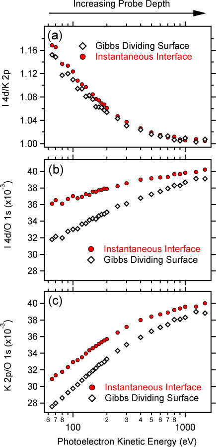
SESSA simulation results of peak-intensity ratios, normalized in each case by ratios of atomic photoionization cross sections, for 2 mol/L KI. a) I 4d/K 2p ratio. b) I 4d/O 1s ratio. c) K 2p/O 1s ratio. Red circles: Instantaneous definition of the interface. Black diamonds: Gibbs dividing surface definition of the interface.

Figure 5a shows the calculated anion-to-cation (I 4d/K 2p) ratio as a function of energy (probe depth). Only minor differences are evident between the two definitions of the interface. At low energies, where the simulation is most sensitive to the composition of the outmost layers of solution, the iodide concentration is enhanced relative to that of potassium, consistent with the density profiles computed directly from the MD simulations shown in Figure 3. This preferential enrichment of iodide (relative to potassium) at the vapor (vacuum)-water interface is now well established by numerous computational and experimental studies,¹⁵ although the driving forces for ion adsorption to the interface are still being debated.⁴¹ The SESSA simulations predict a maximum enhancement in the I 4d/K 2p ratio of 16 % (for a photoelectron energy of 65 eV) based on the atom-density profiles from the MD simulations. This enhancement decreases monotonically with increasing energy until an asymptotic I 4d/K 2p ratio of 1.01 is reached at ≈800 eV. At higher energies, the ratio remains constant.

Figures 5b and 5c show the ion-to-oxygen atomic ratios, I 4d/O 1s and K 2p/O 1s, respectively. The O 1s signal is representative of water. In these ratios, pronounced differences between the two definitions of the interface are evident. In all cases, the ion-to-water ratios decrease relative to their bulk value at 1500 eV as the energy is decreased. This result suggests that, on a relative scale, the concentration of ions near the solution-vapor (or vacuum) interface, for the ID of the chosen experimental conditions (cf. Figure 1), is depleted relative to that in the bulk. This finding seems, at least qualitatively, at odds with the atom-density profiles of Figure 3 where the maximum ion concentrations near the interface peak at densities that exceed those in the bulk. One would perhaps naively expect this ion distribution to manifest itself as an increase in the I 4d/O 1s and K 2p/O 1s ratios as the interface sensitivity of the simulation is increased, not a decrease. This expectation would, however, be at odds with the measured positive surface tension increment of 2 mol/L KI.⁴² The latter result is explained thermodynamically by a net depletion of ions over the entire interfacial length of the system.⁴³ The interfacial length is defined as the depth over which the ion and water density profiles differ from bulk (−1.2 nm for the GDS and −1.5 nm in the instantaneous definition, see Section III C). A simple integration of the density profiles of Figure 3 confirms a net decrease in the ion concentrations over the interfacial lengths. The SESSA simulations capture this decrease.

The more pronounced decrease in the ion to oxygen ratios for the GDS is rationalized qualitatively by analyzing the relative ion depletions between the two interface definitions. In the GDS definition, I⁻ and K⁺ concentrations are depleted (over the −1.2 nm interfacial length) relative to the bulk by 10.6 % and 8.8 %, respectively, whereas the depletions are 8.2 % and 8.4 %, respectively, for the instantaneous definition. These differences are captured by the SESSA simulations, which predict lower signal intensities for the GDS than the instantaneous definition of the interface (Figures 5b and 5c), however, these differences are small and may be difficult to observe in an XPS experiment at a liquid interface.

F. Comparison of SESSA Results with Other Approaches

SESSA is not unique in its ability to calculate XPS signal intensities using atom-density profiles from MD simulations, although it does offer several distinct advantages over the more traditional convolution-integral approach employed by Brown et al.⁴⁴ and Ottosson et al⁷ Here we describe the latter approach and subsequently make a direct comparison with results from SESSA simulations using as example an aqueous solution of 1 mol/L NaI where the density profiles are computed from a MD simulation using the instantaneous definition of the interface.⁴⁰

The XPS signal of atom n can be calculated from MD simulations by integrating the atomic density profile according to¹³

$$I_n(E)={\displaystyle {\int }_0^{+\infty }{\rho }_n(z)}dz+{\displaystyle {\int }_{-\infty }^0{\rho }_n(z)}{e}^{-z/\lambda (E)}dz$$ (2)

where I_n(E) is the XPS signal intensity of the n-th species at the photoelectron kinetic energy E, ρ_n is the density profile of atom n (from the MD simulations), and z is the distance from the interface. The integration limit of zero defines the position of the interface. The first integral in Eq. 2 accounts for the vapor (vacuum)-side of the interface where the total atomic density is low and the electron IMFP term is assumed to vanish: the probability of a photoelectron in this region to undergo an inelastic scattering event is assumed to be zero. The second integral in Eq. 2 accounts for the solution side of the interface. Here photoelectrons have a non-negligible probability to undergo an inelastic scattering event, and the intensity is attenuated with a probability governed by the IMFP. The effects of elastic scattering are neglected in Eq. 2.¹³

The results of performing the integrations of Eq. 2 using the I⁻ and Na⁺ atom-density profiles from the MD simulation of 1 mol/L NaI are shown in Figure 6 (solid blue line). The calculated XP intensities were normalized by the corresponding atomic photoionization cross sections, as before, to give the anion-to-cation ratio, I/Na. The abscissa in Figure 6 has been converted to photoelectron energy using the relation between λ and energy provided by the TPP-2M formula for this solution (see Figure 2, Table 2). The corresponding ratios from the SESSA simulations are also shown in Figure 6 (solid green circles). Pronounced differences in the predicted ion ratios are seen for energies below ≈300 eV, with the SESSA ratios systematically higher than those from Eq. 2. At an energy of 65 eV (where the IMFP is 0.72 nm), a maximum difference of about 12 % is observed.

FIG. 6.

Iodide-to-sodium ratio in 1 mol/L NaI. Green circles: SESSA simulation results (I 4d/K 2p) using atomic-density profiles computed from MD simulations using the instantaneous definition of the interface. Red squares: SESSA simulation results (I 4d/K 2p) in the straight-line approximation (elastic scattering turned off). Solid blue line: Iodide-to-potassium ratio calculated using Eq. 2.

The effect of neglecting elastic scattering events in Eq. 2 can be demonstrated by repeating the SESSA simulations in the straight-line approximation (SLA) where elastic-scattering events are turned off. While these events cannot be turned off in an experiment, it is nonetheless useful here for comparing different theoretical approaches. The results from SESSA simulations with the SLA are shown in Figure 6 as open red squares. The maximum difference between the Traditional Integral and SESSA with SLA results is reduced to a mere 2 %. This result indicates that elastic scattering for this solution may be significant for energies below ≈300 eV.

Other differences between the traditional-integral approach and SESSA are more difficult to quantify and likely account for the remaining 2 %. For instance, each layer in Eq. 2 is assumed to have the same IMFP (as for the bulk of the solution). In SESSA, the IMFP is explicitly calculated for each layer of the solution and we find that IMFPs vary for the near-surface layers (for this 1 mol/L NaI solution) by up to 16% from the bulk values. Specifically, for an energy of 65 eV, the TPP-2M formula predicts an IMFP of 0.83 nm for the layer at a depth of −0.1 nm and 0.72 nm in the bulk.

G. Technical Considerations for SESSA

The band-gap energy (E_g) of the solution is a required input in SESSA for calculation of the IMFP from the TPP-2M equation. In the above SESSA simulations, E_g was assumed to be constant, 7.9 eV. We note, however, that E_g values for water in the literature vary by about ± 1 eV,^45–48 roughly centered around 7.9 eV. Databases for band-gap energies of aqueous electrolyte solutions do not exist. In order to quantify the influence of the solution band-gap energy on the SESSA results, we have carried out additional simulations for 1 mol/L NaI using the instantaneous definition of the interface and E_g values of 6.9 eV, 7.9 eV (as for the previous results) and 8.9 eV. Figure 7a shows plots of the I 4d/Na 2p atomic ratios (derived in the same way as those in Figure 6) as a function of photoelectron energy. Differences in the I 4d/Na 2p ratios do arise for energies below ≈200 eV; however, these differences are small, with variations of only ± 3 % from the results for the E_g = 7.9 eV simulation.

FIG. 7.

Band gap (E_g) and convergence factor (CF) dependencies. a) SESSA simulated I 4d/Na 2p ratios as a function of photoelectron energy for band-gap energies of 6.9 eV (blue squares), 7.9 eV (green circles), and 8.9 eV (red triangles). The simulations were performed for 1 mol/L NaI using the density profiles from MD simulations. b) SESSA simulated I 4d/Na 2p ratios as a function of energy for convergence factors of 10⁻² (blue squares), 10⁻⁴ (green circle), and 10⁻⁶ (red triangles). The system is a semi-infinite structureless slab of 1 mol/L NaI.

The convergence criterion for the SESSA simulation is a user-defined setting. Using a semi-infinite slab of 1 mol/L NaI, the effect of the convergence factor (CF) on the simulated I 4d/Na 2p ratios was assessed (Figure 7b). We find that CFs larger than 10⁻⁶ are insufficient to provide a satisfactory level of statistical accuracy (< 0.5% from the stoichiometric ratio). This level of accuracy is not without computational expense: the series of simulations needed to construct the data set in Figure 7b with a CF of 10⁻⁶ required about 13 minutes (on a personal laptop computer), whereas a CF of 10⁻⁴ required only 1 minute. Simulating an entire 21-layer system, as was done for Figure 5, took ≈45 minutes with a CF of 10⁻⁶.

IV. Conclusions

A straightforward and systematic protocol that uses SESSA for the direct interpretation of MD simulations with XPS signal intensities was presented. Using the TPP-2M predictive formula, the electron IMFP was calculated as a function of photoelectron kinetic energy and shown to depend on solution composition, varying by up to 30 % at 65 eV between pure water and 10 mol/L NaI. The information depth, or surface sensitivity, of the experiment for different photoelectron kinetic energies was calculated using pure water as an example. Even at the lowest kinetic energies routinely employed in XPS experiments from aqueous solutions, 65 eV, the outermost monolayer of solution is responsible for less than half of the total signal intensity. The exacted ion signal intensity ratio (I/K) and ion-to-water signal intensity ratios (I/water and K/water) for 2 mol/L KI were calculated as a function of photoelectron kinetic energy. The corresponding ion ratio for 1 mol/L NaI is compared with that obtained from an ad hoc integral approach widely used within the community. The SESSA results show that the traditional approach for calculating XPS signal intensities from MD atom-density profiles systematically underestimates the preferential enhancement of the anion (over the cation) at the vapor (vacuum)-aqueous electrolyte interface. This difference can be primarily traced to the neglect of elastic-scattering events in the traditional approach.

SESSA is straightforward to use and shows promise for enabling quantitative comparisons between energy-dependent X-ray photoelectron spectroscopy signal intensities and the results of MD simulations. In on-going work, we are carrying out a systematic comparison of MD/SESSA simulation results with experimental data on a variety of aqueous salt solutions.

References

- 1.Powell CJ, Jablonski A. Nucl Instrum Meth A. 2009;601(1–2):54–65. [Google Scholar]
- 2.Powell CJ, Jablonski A. J Electron Spectrosc. 2010;178:331–346. [Google Scholar]
- 3.Tanuma S, Powell CJ, Penn DR. Surf Interface Anal. 1994;21(3):165–176. [Google Scholar]
- 4.Seah MP. Surf Interface Anal. 2012;44(4):497–503. [Google Scholar]
- 5.Powell CJ, Jablonski A. J Phys Chem Ref Data. 1999;28(1):19–62. [Google Scholar]
- 6.Suzuki YI, Nishizawa K, Kurahashi N, Suzuki T. Phys Rev E. 2014;90(1):010302(R). doi: 10.1103/PhysRevE.90.010302. [DOI] [PubMed] [Google Scholar]
- 7.Ottosson N, Faubel M, Bradforth SE, Jungwirth P, Winter B. J Electron Spectrosc. 2010;177(2–3):60–70. [Google Scholar]
- 8.Thurmer S, Seidel R, Faubel M, Eberhardt W, Hemminger JC, Bradforth SE, Winter B. Phys Rev Lett. 2013;111(17):173005. doi: 10.1103/PhysRevLett.111.173005. [DOI] [PubMed] [Google Scholar]
- 9.Emfietzoglou D, Kyriakou I, Abril I, Garcia-Molina R, Petsalakis ID, Nikjoo H, Pathak A. Nucl Instrum Meth B. 2009;267(1):45–52. [Google Scholar]
- 10.Jordan I, Redondo AB, Brown MA, Fodor D, Staniuk M, Kleibert A, Worner HJ, Giorgi JB, van Bokhoven JA. Chem Commun. 2014;50(32):4242–4244. doi: 10.1039/c4cc00720d. [DOI] [PubMed] [Google Scholar]
- 11.Ghosal S, Hemminger JC, Bluhm H, Mun BS, Hebenstreit ELD, Ketteler G, Ogletree DF, Requejo FG, Salmeron M. Science. 2005;307(5709):563–566. doi: 10.1126/science.1106525. [DOI] [PubMed] [Google Scholar]
- 12.Ghosal S, Brown MA, Bluhm H, Krisch MJ, Salmeron M, Jungwirth P, Hemminger JC. J Phys Chem A. 2008;112(48):12378–12384. doi: 10.1021/jp805490f. [DOI] [PubMed] [Google Scholar]
- 13.Cheng MH, Callahan KM, Margarella AM, Tobias DJ, Hemminger JC, Bluhm H, Krisch MJ. J Phys Chem C. 2012;116(7):4545–4555. [Google Scholar]
- 14.Krisch MJ, D’Auria R, Brown MA, Tobias DJ, Hemminger JC, Ammann M, Starr DE, Bluhm H. J Phys Chem C. 2007;111(36):13497–13509. [Google Scholar]
- 15.Jungwirth P, Tobias DJ. Chem Rev. 2006;106(4):1259–1281. doi: 10.1021/cr0403741. [DOI] [PubMed] [Google Scholar]
- 16.Smekal W, Werner WSM, Powell CJ. Surf Interface Anal. 2005;37(11):1059–1067. [Google Scholar]
- 17.Werner WSM, Smekal W, Powell CJ. NIST Database for the Simulation of Electron Spectra for Surface Analysis, Version 2.0, Standard Reference Data program Database 100. Department of Commerce, National Institute of Standards and Technology; Gaithersburg, Maryland: 2014. [Google Scholar]
- 18.Van der Spoel D, Lindahl E, Hess B, Groenhof G, Mark AE, Berendsen HJC. J Comput Chem. 2005;26(16):1701–1718. doi: 10.1002/jcc.20291. [DOI] [PubMed] [Google Scholar]
- 19.Vangunsteren WF, Berendsen HJC. Angewandte Chemie-International Edition. 1990;29(9):992–1023. [Google Scholar]
- 20.Berendsen HJC, Vanderspoel D, Vandrunen R. Comput Phys Commun. 1995;91(1–3):43–56. [Google Scholar]
- 21.Lindahl E, Hess B, van der Spoel D. J Mol Model. 2001;7(8):306–317. [Google Scholar]
- 22.Hess B, Kutzner C, van der Spoel D, Lindahl E. J Chem Theory Comput. 4(3):435–447. doi: 10.1021/ct700301q. [DOI] [PubMed] [Google Scholar]
- 23.Bussi G, Donadio D, Parrinello M. J Chem Phys. 2007;126(1) doi: 10.1063/1.2408420. [DOI] [PubMed] [Google Scholar]
- 24.Horinek D, Herz A, Vrbka L, Sedlmeier F, Mamatkulov SI, Netz RR. Chem Phys Lett. 2009;479(4–6):173–183. [Google Scholar]
- 25.Berendsen HJ, Grigera JR, Straatsma TP. J Phys Chem-Us. 1987;91(24):6269–6271. [Google Scholar]
- 26.Essmann U, Perera L, Berkowitz ML, Darden T, Lee H, Pedersen LG. J Chem Phys. 1995;103(19):8577–8593. [Google Scholar]
- 27.Miyamoto S, Kollman PA. J Comput Chem. 1992;13(8):952–962. [Google Scholar]
- 28.Washburn EW. International Critical Tables of Numerical Data, Physics, Chemistry, and Technology. McGraw-Hill; New York: 1928. [Google Scholar]
- 29.ON Sohnel P. Densities of Aqueous Solutions of Inorganic Substances. Elsevier Science; Amsterdam: 1985. [Google Scholar]
- 30.Willard AP, Chandler D. J Phys Chem B. 2010;114(5):1954–1958. doi: 10.1021/jp909219k. [DOI] [PMC free article] [PubMed] [Google Scholar]
- 31.Stern AC, Baer MD, Mundy CJ, Tobias DJ. J Chem Phys. 2013;138(11):114709. doi: 10.1063/1.4794688. [DOI] [PubMed] [Google Scholar]
- 32.Tanuma S, Powell CJ, Penn DR. Surf Interface Anal. 2005;37(1):1–14. [Google Scholar]
- 33.Brown MA, Redondo AB, Jordan I, Duyckaerts N, Lee MT, Ammann M, Nolting F, Kleibert A, Huthwelker T, Machler JP, Birrer M, Honegger J, Wetter R, Worner HJ, van Bokhoven JA. Rev Sci Instrum. 2013;84(7):073904. doi: 10.1063/1.4812786. [DOI] [PubMed] [Google Scholar]
- 34.Yeh JJ, Lindau I. Atom Data Nucl Data. 1985;32(1):1–155. [Google Scholar]
- 35.ISO 18115:2013. Surface chemical analysis - Vocabulary - Part 1. International Organization for Standardization; Geneva: 2013. [Google Scholar]
- 36.Jablonski A, Powell CJ. J Vac Sci Technol A. 2009;27(2):253–261. [Google Scholar]
- 37.This parameter is defined as the ratio of the IMFP to the sum of the IMFP and the transport mean free path (TMFP). The TMFP is the inverse product of the density of atoms or molecules and the transport cross section that is calculated from the differential cross section for elastic scattering of electrons by the atoms or molecules.
- 38.Tao F, Grass ME, Zhang YW, Butcher DR, Renzas JR, Liu Z, Chung JY, Mun BS, Salmeron M, Somorjai GA. Science. 2008;322(5903):932–934. doi: 10.1126/science.1164170. [DOI] [PubMed] [Google Scholar]
- 39.Tissot H, Olivieri G, Gallet JJ, Bournel F, Silly MG, Sirotti F, Rochet F. J Phys Chem C. 2015;119(17):9253–9259. [Google Scholar]
- 40.See supplementary material at [URL] for the detailed composition of each layer used as SESSA input parameters for 2 MKI and 1 M NaI in the instantaneous interface representation and 2 M KI in the GDS rapresentation. For 1 M NaI the MD simulation results are also shown.
- 41.Tobias DJ, Stern AC, Baer MD, Levin Y, Mundy CJ. Annu Rev Phys Chem. 2013;64:339–359. doi: 10.1146/annurev-physchem-040412-110049. [DOI] [PubMed] [Google Scholar]
- 42.Ali K, Shah AUHA, Bilal S, Shah AUHA. Colloid Surface A. 2009;337(1–3):194–199. [Google Scholar]
- 43.D’Auria R, Tobias DJ. J Phys Chem A. 2009;113(26):7286–7293. doi: 10.1021/jp810488p. [DOI] [PubMed] [Google Scholar]
- 44.Brown MA, Winter B, Faubel M, Hemminger JC. J Am Chem Soc. 2009;131(24):8354–8355. doi: 10.1021/ja901791v. [DOI] [PubMed] [Google Scholar]
- 45.Goulet T, Bernas A, Ferradini C, Jay-Gerin JP. Chem Phys Lett. 1990;170(5–6):492–496. [Google Scholar]
- 46.Bernas A, Ferradini C, Jay-Gerin JP. Chem Phys. 1997;222(2–3):151–160. [Google Scholar]
- 47.Coe JV, Earhart AD, Cohen MH, Hoffman GJ, Sarkas HW, Bowen KH. J Chem Phys. 1997;107(16):6023–6031. [Google Scholar]
- 48.Coe JV. Int Rev Phys Chem. 2001;20(1):33–58. [Google Scholar]
Associated Data
This section collects any data citations, data availability statements, or supplementary materials included in this article.