Linear mixed model for heritability estimation that explicitly addresses environmental variation

Abstract

The linear mixed model (LMM) is now routinely used to estimate heritability. Unfortunately, as we demonstrate, LMM estimates of heritability can be inflated when using a standard model. To help reduce this inflation, we used a more general LMM with two random effects—one based on genomic variants and one based on easily measured spatial location as a proxy for environmental effects. We investigated this approach with simulated data and with data from a Uganda cohort of 4,778 individuals for 34 phenotypes including anthropometric indices, blood factors, glycemic control, blood pressure, lipid tests, and liver function tests. For the genomic random effect, we used identity-by-descent estimates from accurately phased genome-wide data. For the environmental random effect, we constructed a covariance matrix based on a Gaussian radial basis function. Across the simulated and Ugandan data, narrow-sense heritability estimates were lower using the more general model. Thus, our approach addresses, in part, the issue of “missing heritability” in the sense that much of the heritability previously thought to be missing was fictional. Software is available at https://github.com/MicrosoftGenomics/FaST-LMM.

An important causal question comes from the age-old debate about nature versus nurture. For any phenotype such as height or intelligence quotient, how much of the phenotype is inherited and how much is determined by environment? This question was made precise by Fisher (1) and Wright (2) almost a century ago: Given observations of a phenotype from a population of individuals, what is the fraction of variance of the phenotype that is caused by inherited factors relative to the total variance of the phenotype due to both inherited and environmental factors? This fraction, termed “heritability,” has been the subject of intense study across various phenotypes and populations since it was defined. Note that, in contrast to how some interpret the informal question around the nature-versus-nurture debate, heritability is not an absolute quantity but rather a quantity relative to a given population. For example, a phenotype in a population where environmental factors have large variation will have a smaller heritability than in an otherwise similar population where environmental factors have a small variation.

Over the years, many approaches have been developed to estimate heritability from data (3, 4). Here, we concentrate on an approach made possible by the recent ability to sequence genomes at a modest cost (5, 6). The approach uses a linear mixed model (LMM), a form of multivariate regression of the genomic and environmental factors on the phenotype, which we examine in detail in the next section.

In the standard LMM approach, the effects of environmental factors on the phenotype are modeled as noise. Specifically, the phenotype of each individual is assumed to be the sum of two random effects, one based on genomic factors and one based on environmental factors, where the latter is assumed to be mutually independent across individuals. As we shall see, this model for environmental effects can lead to inflated estimates of heritability.

To avoid this inflation, we could measure and model environmental effect explicitly (e.g., ref. 7). Unfortunately, in most circumstances there are many environmental factors to be measured. Furthermore, some environmental factors may be unrecognized and consequently are unmeasurable. In this work, we investigate the use of an easy-to-measure surrogate for environmental factors—namely, spatial location. We show how this surrogate can be incorporated into the LMM as an additional random effect. We investigate our more general model with simulated data and with data from a Ugandan cohort of about 5,000 individuals.

Results

Heritability Estimation.

First, let us consider a standard approach for estimating heritability using an LMM (6, 8). The estimate is based on observations consisting of y, an $N\times 1$ vector of phenotypes for the N individuals, and X, an $N\times M$ matrix of causal genomic variants for the N individuals and M variants. Note that it is customary to normalize the causal variants so that each one has a mean of zero and an SD of one across individuals. Given these observations, we model y as a multivariate linear regression on X:

$$\mathit{y}\sim \mathcal{N}\left(\mathbf{\mu }+\mathbf{X}\mathit{\beta }\text{;}{\sigma }_r^2\mathbf{I}\right),$$ [1]

where $\mathbf{\mu }$ is an $N\times 1$ vector of offsets that can include the effects of covariates, $\mathit{\beta }$ is the $M\times 1$ vector of linear weights relating the corresponding variants to the phenotype, $\mathbf{I}$ is the $N\times N$ identity matrix, and ${\sigma }_r^2$ is the residual variance of the multivariate normal distribution denoted by $\mathcal{N}$(.; .). In addition, we assume that the elements of $\mathit{\beta }$ are mutually independent, each having a normal distribution:

$${\mathit{\beta }}_i\sim \mathcal{N}\left(0\text{;}\hspace{0.17em}\frac{{\sigma }_g^2}{M}\right),\hspace{0.17em}i=1,\dots ,\hspace{0.17em}M.$$ [2]

Plugging Eq. 2 into Eq. 1 and integrating out $\mathit{\beta }$, we obtain

$$\mathit{y}\sim \mathcal{N}\left(\mathbf{\mu }\text{;}{\sigma }_g^2\frac{1}{M}\mathbf{X}{\mathbf{X}}^{\text{T}}+{\sigma }_r^2\mathbf{I}\right).$$ [3]

Model 3 is known as a linear mixed model with a random effect having the covariance matrix ${\mathbf{K}}_{\mathbf{c}\mathbf{a}\mathbf{u}\mathbf{s}\mathbf{a}\mathbf{l}}=\frac{1}{\mathit{M}}\mathbf{X}{\mathbf{X}}^{\text{T}}$ (9). It is also known as a Gaussian process with a linear covariance (or kernel) function (10, 11). Note that element i,j of ${\mathbf{K}}_{\mathbf{c}\mathbf{a}\mathbf{u}\mathbf{s}\mathbf{a}\mathbf{l}}$ is the dot product ${\displaystyle \sum _{k=1}^M}{\mathbf{X}}_{ik}{\mathbf{X}}_{jk}.$ The parameters of this model are typically fit by maximizing the restricted maximum likelihood (REML) of the data.

Narrow sense heritability, denoted $h^2,$ is the fraction of the variance of $\mathit{y}$ due to the genomic component. Given this model and the assumption that genomic variants are mutually independent, it follows that

$$h^2=\frac{{\sigma }_g^2\hspace{0.17em}}{{\sigma }_g^2+{\sigma }_r^2}.$$ [4]

Note that narrow-sense heritability accounts only for additive genomic effects. Genomic effects can also exhibit nonlinear interactions among each other (known as epistasis) and exhibit dominance, neither of which is captured in the model of Eq. 3. The term “heritability” without the modifier “narrow sense” is typically reserved for the quantity that includes all genomic effects. Herein, for simplicity, we will concentrate on the estimation of narrow-sense heritability although, as we mention later, our approach can be extended to estimate more general quantities.

In practice, we do not know which genomic variants are causal, so we use an approximation for ${\mathbf{K}}_{\mathbf{c}\mathbf{a}\mathbf{u}\mathbf{s}\mathbf{a}\mathbf{l}}$. One commonly used approximation—and one we will use in this work—is ${\mathbf{K}}_{\mathbf{I}\mathbf{B}\mathbf{D}}$, where element (i,j) is the fraction of the genome shared identical by descent (IBD) among individuals i and j (6). That is, we use the model

$$\mathit{y}\sim \mathcal{N}\left(\mathbf{\mu }\text{;}{\sigma }_g^2{\mathbf{K}}_{\mathbf{I}\mathbf{B}\mathbf{D}}+{\sigma }_r^2\mathbf{I}\right).$$

As noted in the introduction, the standard LMM represents environmental effects as simple Gaussian noise. Here, let us consider a more general model for environmental effects based on the spatial location of individuals. Specifically, consider the addition of a random effect with covariance matrix ${\mathbf{K}}_{\mathbf{l}\mathbf{o}\mathbf{c}}$:

$$\mathit{y}\sim \mathcal{N}\left(\mathbf{\mu }\text{;}{\sigma }_g^2{\mathbf{K}}_{\mathbf{I}\mathbf{B}\mathbf{D}}+{\sigma }_e^2{\mathbf{K}}_{\mathbf{l}\mathbf{o}\mathbf{c}}+{\sigma }_r^2\mathbf{I}\right).$$ [5]

Assuming the genomic variants and spatial locations are mutually independent, we get a new estimate for narrow-sense heritability given by

$$h^2=\frac{{\sigma }_g^2\hspace{0.17em}}{{\sigma }_g^2+{\sigma }_e^2+{\sigma }_r^2}.$$ [6]

This model also allows us to estimate the fraction of variance of $\mathit{y}$ due to the location component, denoted $e^2$:

$$e^2=\frac{{\sigma }_e^2\hspace{0.17em}}{{\sigma }_g^2+{\sigma }_e^2+{\sigma }_r^2}.$$ [7]

In our analysis of the Ugandan cohort, we use ${\mathbf{K}}_{\mathbf{l}\mathbf{o}\mathbf{c}}(i,j)=\text{exp}\{-{(d_{ij}/\alpha )}^2\}$, where $d_{ij}$ is the distance between individuals i and j, and α is a scaling parameter. Intuitively, the inclusion of ${\mathbf{K}}_{\mathbf{l}\mathbf{o}\mathbf{c}}$ captures the notion that individuals physically closer to each other are more likely to be influenced by the same environmental factors and hence more likely to have similar phenotypes. Using other types of proximity—for example, social proximity—is also possible, but here we consider only physical proximity. The exponential form we use for ${\mathbf{K}}_{\mathbf{l}\mathbf{o}\mathbf{c}}(i,j)$ is known as a Gaussian radial basis function and is often used in spatial analyses (10, 11). (We also tried the radial basis function $\text{exp}\{-(d_{ij}/\alpha )\}$ but found it difficult to estimate $\alpha$ accurately.) The parameter α can be thought of as the spatial range of the environmental effect. The larger the value for α, the larger the range or extent of the effect. As in the standard case, we fit all parameters, now including ${\sigma }_e^2$ and α, with REML.

Recall that the standard LMM follows from modeling the phenotype as a regression on genomic variants. Similarly, Eq. 5 can be interpreted as the result of modeling the phenotype as a multivariate regression on both genomic variants and spatial location. In particular, Mercer’s theorem (10, 11) states that, if K(z_i,z_j) is a continuous symmetric positive semidefinite function to $\mathrm{ℝ}$ from z_i and z_j each in a compact Hausdorff space, then there exists a set of functions ϕ_k(z), k = 1,…,∞, such that K(z_i,z_j) is equal to the dot product ${\displaystyle \sum _{k=1}^{\infty }}{\varphi }_k\left(z_i\right){\varphi }_k\left(z_j\right)$. Identifying z_i as the spatial location of individual i and K(z_i,z_j) as element i,j in ${\mathbf{K}}_{\mathbf{l}\mathbf{o}\mathbf{c}}$, it follows that the inclusion of ${\mathbf{K}}_{\mathbf{l}\mathbf{o}\mathbf{c}}$ in Eq. 5 is equivalent to conditioning on spatial features ϕ_k(z_i), i = 1,…,N, k = 1,…,∞. We note that the Gaussian radial basis function is guaranteed to be positive semidefinite.

Finally, let us consider nonlinear interactions between genomic and environmental components. We can model some of these interactions by introducing a third random effect to the LMM:

$$\mathit{y}\sim \mathcal{N}\left(\mathbf{\mu }\text{;}{\sigma }_g^2{\mathbf{K}}_{\mathbf{I}\mathbf{B}\mathbf{D}}+{\sigma }_e^2{\mathbf{K}}_{\mathbf{l}\mathbf{o}\mathbf{c}}+{\sigma }_{gxe}^2{\mathbf{K}}_{\mathbf{G}\mathbf{x}\mathbf{E}}+{\sigma }_r^2\mathbf{I}\right),$$ [8]

producing an estimate of the fraction of variance of $\mathit{y}$ due to the interaction component given by

$$gx{e}^2=\frac{{\sigma }_{gxe}^2\hspace{0.17em}}{{\sigma }_g^2+{\sigma }_e^2+{\sigma }_{gxe}^2+{\sigma }_r^2}.$$ [9]

We use a particular form for ${\mathbf{K}}_{\mathbf{G}\mathbf{x}\mathbf{E}}$ where element i,j is the product of elements i,j from ${\mathbf{K}}_{\mathbf{c}\mathbf{a}\mathbf{u}\mathbf{s}\mathbf{a}\mathbf{l}}$ and ${\mathbf{K}}_{\mathbf{l}\mathbf{o}\mathbf{c}}$ (i.e., the Handamard product of ${\mathbf{K}}_{\mathbf{c}\mathbf{a}\mathbf{u}\mathbf{s}\mathbf{a}\mathbf{l}}$ and ${\mathbf{K}}_{\mathbf{l}\mathbf{o}\mathbf{c}}$). Using the nomenclature we have defined, it follows that element i,j of$\hspace{0.17em}$ ${\mathbf{K}}_{\mathbf{G}\mathbf{x}\mathbf{E}}$ is given by ${\displaystyle \sum _{k=1}^M}{\displaystyle \sum _{l=1}^{\infty }}{X}_{ik}{\varphi }_l\left(z_i\right)X_{jk}{\varphi }_l\left(z_j\right)$. Consequently, inclusion of ${\mathbf{K}}_{\mathbf{G}\mathbf{x}\mathbf{E}}$ into the LMM is equivalent to conditioning on the features X_ik ϕ_l(z_i), i = 1,…,N, k = 1,…,M, l = 1,…,∞. Product features such as these are often used to model nonlinear interactions (12). In our analysis of the Ugandan cohort, we use this instance of ${\mathbf{K}}_{\mathbf{G}\mathbf{x}\mathbf{E}}$, except we replace ${\mathbf{K}}_{\mathbf{c}\mathbf{a}\mathbf{u}\mathbf{s}\mathbf{a}\mathbf{l}}$ with ${\mathbf{K}}_{\mathbf{I}\mathbf{B}\mathbf{D}}$ as an approximation.

We note that the standard model given by Eq. 3 is nested in the model given by Eq. 5, which in turn is nested in the model given by Eq. 8.

Heritability Analysis on Simulated Data.

We first applied our approach to the analysis of simulated data. We generated from the Balding–Nichols model (13) with a 50:50 population ratio, a baseline minor allele frequency (MAF) sampled uniformly from [0.05, 0.5], and a value for Wright’s F_ST equal to 0.1. We generated a spatial location for each individual by sampling randomly from one of two spherical Gaussian distributions with SD 625,000 and separation between Gaussian centers equal to 4 × 625,000. This procedure produced a distribution of spatial locations similar to the real data and satisfied an assumption underlying Eqs. 6 and 7 that genomic variants and spatial locations are independent. We next generated the phenotype using Eq. 5 with ${\mathbf{K}}_{\mathbf{I}\mathbf{B}\mathbf{D}}$ replaced with ${\mathbf{K}}_{\mathbf{c}\mathbf{a}\mathbf{u}\mathbf{s}\mathbf{a}\mathbf{l}}$, and with ${\sigma }_g^2={\sigma }_e^2={\sigma }_r^2=1,$ and α = 4 × 625,000. We generated 50 datasets and then, for each one, computed uncorrected and corrected heritability estimates, based on Eqs. 3 and 5, respectively, with ${\mathbf{K}}_{\mathbf{I}\mathbf{B}\mathbf{D}}$ replaced with ${\mathbf{K}}_{\mathbf{c}\mathbf{a}\mathbf{u}\mathbf{s}\mathbf{a}\mathbf{l}}.$ For each dataset, we generated 1,000 causal SNPs for 5,000 individuals to mimic the real data.

The estimates of $h^2$ and $e^2$ based on the corrected model are unbiased, having mean (± SE) of 0.33 ± 0.01 and 0.35 ± 0.02, respectively. In contrast, the estimates of $h^2$ based on the standard or uncorrected model were inflated (0.42 ± 0.01). This inflation is not unexpected, because the “signal” produced by the spatial random effect needs to be accounted for by either the genomic random effect or the noise component, and there is no reason to expect that the noise component would account for all of it. Any leakage of the signal arising from the spatial random effect to the genomic random effect would yield inflated estimates of heritability. That is, model misspecification can lead to substantial bias in heritability estimates.

As mentioned, Eqs. 6 and 7 were derived under an assumption that genomic and spatial factors are independent. In practice, however, this assumption may not hold. To investigate the robustness of these estimates to nonindependence, we modified the above data-generation procedure to create a dependence between genomic and spatial variation. In particular, the spatial locations of all individuals from the same Balding–Nichols population were drawn from the same spherical Gaussian. Despite this relatively strong dependence, estimates of $h^2$ (corrected) and $e^2$ remained unbiased (0.33 ± 0.01 and 0.35 ± 0.02, respectively). Uncorrected estimates of $h^2$ were similarly inflated in the presence of dependence (0.46 ± 0.01).

Sample code for these experiments in the form of an iPython notebook can be found in SI Appendix.

Heritability Analysis on the Ugandan Cohort.

We next applied our approach to an analysis of a Ugandan cohort (Methods) across 34 phenotypes including anthropometric indices, blood factors, glycemic control, blood pressure, lipid tests, and liver function tests. A description of phenotypes can be found in Table 1. Not unexpectedly, heritability estimates varied widely, with corrected estimates ranging from 0.55 for mean platelet volume (MPV) to 0.10 for levels of alkaline phosphatase (Table 2).

Table 1.

A description of the phenotypes measured in the Ugandan cohort

Phenotype	Category	Description
BMI	Anthropometric index	Body mass index
Height	Anthropometric index	Height
HIP	Anthropometric index	Hip circumference
Waist	Anthropometric index	Waist circumference
Weight	Anthropometric index	Weight
WHR	Anthropometric index	Waist–hip ratio
Basophils	Blood factor	Basophil count
Eosinophils	Blood factor	Eosinophil count
Hematocrit	Blood factor	Hematocrit
Hemoglobin	Blood factor	Hemoglobin
Lymphocytes	Blood factor	Lymphocyte count
MCH	Blood factor	Mean corpuscular hemoglobin
MCHC	Blood factor	Mean corpuscular hemoglobin concentration
MCV	Blood factor	Mean corpuscular volume
Monocytes	Blood factor	Monocyte count
MPV	Blood factor	Mean platelet volume
Neutrophils	Blood factor	Neutrophil count
Platlets	Blood factor	Platelet count
RBC dstr width	Blood factor	Red blood cell distribution width
RBCs	Blood factor	Red blood cell count
WBC	Blood factor	White blood cell count
DBP	Blood pressure	Diastolic blood pressure
SBP	Blood pressure	Systolic blood pressure
HbA1c2	Glycemic control	HbA1c2
Cholesterol	Lipid test	Total cholesterol
HDL	Lipid test	High-density lipoprotein
LDL	Lipid test	Low-density lipoprotein
Triglycerides	Lipid test	Triglycerides
Alanine	Liver function	Alanine aminotransferase test
Albumin	Liver function	Serum albumin test
Alkaline	Liver function	Alkaline phosphatase test
Aspartate	Liver function	Aspartate aminotransferase test
Bilirubin	Liver function	Bilirubin
Gamma	Liver function	Gamma-glutamyl transpeptidase test

Table 2.

Results from an analysis of the Ugandan cohort

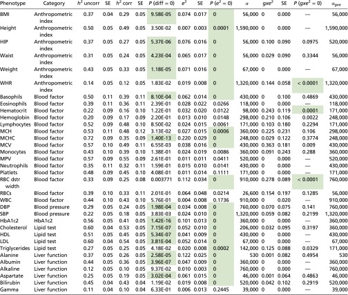Uncorrected (uncorr) and corrected (corr) heritability estimates and estimates of $e^2$ and $gx{e}^2$ are shown along with their SEs. All SEs were computed from a 500-group jackknife. The P value testing the null that there is no difference between the uncorrected and corrected heritability estimates was a based on a two-sided test from a 500-group jackknife on the difference. The P values testing the null hypotheses that ${\sigma }_e^2$ = 0 and ${\sigma }_{gxe}^2$ = 0 were based on a one-sided test with 10,000 permutations (Methods). The values for α are in arbitrary units. The cells in green indicate statistical significance after Bonferroni correction. Columns 2–9 and 10–13 correspond to an analysis without and with the gxe variance component, respectively.

Consistent with our studies on simulated data, uncorrected heritability estimates were inflated. The inflation was significant for 14 of the 34 phenotypes (Fig. 1). In addition, 23 phenotypes had a value for $e^2$ significantly greater than zero (Table 2). In general, we would expect that $e^2>0$ would be a necessary but not sufficient condition for a difference in corrected and uncorrected heritabilities. Consistent with this expectation, these 23 phenotypes are a superset of the 14. We note that for 11 of the phenotypes, $e^2$ was not significantly greater than zero. In these cases, the standard model, which is nested in our more general model, provided an adequate model for heritability.

Fig. 1.

Uncorrected and corrected estimates of narrow-sense heritability for phenotypes from the Ugandan cohort. The height of the blue and red bar combined corresponds to the uncorrected heritability estimate (based on Eq. 3). The height of the blue bar corresponds to the corrected heritability estimate (based on Eq. 5). Asterisks denote differences that are statistically significant after Bonferroni correction based on a two-sided test on the difference between uncorrected and corrected estimates from a 500-group jackknife.

For each phenotype, we were also able to determine the geographical range of the environmental effect (i.e., the optimized value of the scaling parameter α), which varied by more than three orders of magnitude across the phenotypes (Table 2).

Interestingly, corrections were most substantial for anthropometric indices, lipid tests, and measures of liver function. This pattern, which may or may not be real, is under investigation. We are also working to identify specific environmental effects responsible for the large heritability corrections. For the phenotype mean corpuscular hemoglobin concentration (MCHC), which had the largest correction, we ruled out several factors as substantial sources of environmental effects. In particular, elevation was excluded because the terrain of the study is essentially flat. Also, the heritability corrections were about the same for males and females, which we would not expect if iron was a contributor. In addition, heritability correction remained high when MCHC was adjusted for primary occupation and alcohol consumption. On examining this spatial effect in more detail, we found that MCHC varied substantially from one village to the next. Previously, we have shown substantial variation in urbanicity indicators among these villages (14), consistent with this observation. We further explored the possibility of this spatial variation arising because villages were sampled in batches over time. We observed significant improvement in the model on inclusion of sampling date as a covariate. Nonetheless, even with this inclusion, the ratio of uncorrected to corrected $h^2$ remained almost the same. Our findings suggest that environmental factors influencing traits are complex, and understanding them will require further exploration in future studies with the relevant environmental phenotypic data.

Finally, we estimated the variance of the phenotypes due to interactions between genomic and environmental components, fitting the three random effects corresponding to ${\mathbf{K}}_{\mathbf{I}\mathbf{B}\mathbf{D}}$, ${\mathbf{K}}_{\mathbf{l}\mathbf{o}\mathbf{c}}$, and ${\mathbf{K}}_{\mathbf{G}\mathbf{x}\mathbf{E}}$ simultaneously. The variance ${\sigma }_{gxe}^2$ for three phenotypes—hematocrit, red-blood-cell distribution width, and waist-to-hip ratio—was significantly greater than zero (Table 2).

Discussion

We have introduced an LMM approach that includes explicit representation of spatial location in estimates of narrow-sense heritability. Spatial location is presumably a surrogate for (some) environmental effects and, unlike many environmental variables, is easy to measure. On simulated data, we have shown that estimates of heritability based on the more general model seem to be unbiased, whereas the estimates based on the standard model are inflated for some phenotypes. Similarly, in an analysis of 34 phenotypes in a Ugandan cohort, we have found that the uncorrected estimates of heritability based on the standard model are inflated relative to corrected estimates based on the new model. Furthermore, on simulated data, we have shown that the degree of bias is not substantially influenced by the absence or presence of dependence between genomic and environmental factors. Overall, we have demonstrated that estimates of heritability can depend on the nature of environmental variation.

The corrections were substantial, emphasizing the importance of explicitly modeling environmental effects in the estimation of heritability. Furthermore, the amount of inflation varied considerably across the 34 phenotypes, being the greatest for anthropometric indices, lipid tests, and measures of liver function. Presumably in this study, and perhaps in others, spatially related environmental factors affect these phenotypes more. A better understanding of differential bias across traits will require further exploration in cohorts with the relevant environmental phenotypic data.

Our approach has been applied only to the analysis of simulated data and the Ugandan cohort. Nonetheless, if the inflation seen here is typical, then this work offers a new interpretation of results of genome-wide association studies (GWAS). In particular, GWAS studies have so far revealed consistent “missing heritability,” where the variability explained by SNPs identified as associated with a phenotype has been far less than the variability identified in heritability estimates (15). This work suggests that much of this missing heritability was not missing in the first place.

An important lesson from this work is that model misspecification can lead to substantial bias in heritability estimates. Because our use of the Gaussian radial basis function to quantify spatial similarity is itself likely to be misspecified, our corrected estimates of heritability on the Ugandan cohort may remain biased to some degree. Thus, we are investigating alternative similarity functions and methods to select the best one based on data.

We are also investigating modifications to the model beyond the form of the similarity function. One potential modification is based on the well-known fact that narrow-sense heritability estimates will be inflated when the data contains closely related individuals due to effects of dominance and epistasis (3, 4). This inflation could be mitigated by including variance components reflecting IBD2 (both alleles shared) (e.g., see ref. 16) and epistasis (e.g., ref. 17). In addition, one could include a variance component based on whether individuals are in the same household or a variance component based whether individuals are in the same village. As another example, one could include a variance component based on social connectivity, which is known to affect various phenotypes, including obesity (18).

Finally, in addition to heritability estimation, LMMs are also commonly used for identifying associations between genomic variants and phenotypes (e.g., genome-wide association studies) and for prediction. The LMM models described in this work could be applied to these applications as well.

Methods

We collected data for 5,000 individuals from nine ethnolinguistic groups from the General Population Cohort (GPC), Uganda (19). The GPC is a population-based open cohort study established in 1989 by the Medical Research Council in collaboration with the Uganda Virus Research Institute (UVRI) to examine trends in prevalence and incidence of HIV infection and their determinants. Samples were collected from individuals during a survey from the study area located in southwestern Uganda in Kyamulibwa subcounty of Kalungu district, ∼120 km from Entebbe town. The study area is divided into villages defined by administrative boundaries varying in size from 300 to 1,500 residents and includes families living within households. Data on health and lifestyle were collected using a standard individual questionnaire, blood samples obtained, and biophysical measurements taken, when necessary, as described previously (19). Spatial location was recorded in Global Positioning System coordinates. The measurements were translated and scaled to mitigate privacy concerns.

The GPC study was approved by the Uganda Virus Research Institute, Science and Ethics Committee (Ref. GC/127/10/10/25), the Uganda National Council for Science and Technology (Ref. HS 870), and the U.K. National Research Ethics Service, Research Ethics Committee (Ref. 11/H0305/5). Care was taken to obtain genuine informed consent from participants, including the use of reliable intermediaries as appropriate to ensure that the implications of participation were fully understood. Consent forms were translated from English into Luganda and checked for accuracy. The Lugandan translation was given to participants to read themselves, or was read out aloud to them by study staff. Participants could choose to consent to all, or just selected parts, of the survey. The informed consent of participants was obtained with a signature on the consent forms or a thumb print if the participant was unable to write. For participants aged 13–17 y, parental consent as well as child formal assent were collected. The immediate counter signature of a witness was then obtained. The APCDR committees are responsible for curation, storage, and sharing of the data under managed access. The genomic data have been deposited at the European Genome-phenome Archive (EGA, https://www.ebi.ac.uk/ega/) under accession number EGAS00001001558. Requests for access to phenotype data may be directed to data@apcdr.org.

We genotyped 5,000 samples from the Ugandan Survey on the Illumina HumanOmni 2.5M BeadChip array at the Wellcome Trust Sanger Institute. Sequenom quality control and gender checks were carried out before genotyping. A total of 2,314,174 autosomal and 55,208 X-chromosome markers were genotyped on the HumanOmni2.5–8 chip. Of these, 39,368 autosomal markers were excluded because they did not pass the quality thresholds for the SNP called proportion (<97%, 25,037 SNPs) and Hardy–Weinberg equilibrium (HWE) (P < 10⁻⁸, 14,331 SNPs). HWE testing was only carried out on the founders for autosomes, and female unrelated individuals for the X chromosome defined by an IBD threshold <0.10 as estimated by PLINK. A total of 91 samples were dropped during sample quality control because they did not pass the quality thresholds for proportion of samples called (>97%) or heterozygosity (outliers: mean ± 3 SD), or the gender inferred from the X-chromosome data did not match the supplied gender. Three additional samples were dropped because of high relatedness (i.e., IBD >0.90). Principal component analysis was carried out on unrelated individuals projecting onto related individuals, for SNPs LD pruned at an r² threshold of 0.2, with a MAF threshold of >5%. No samples were identified as population/ancestry outliers based on this analysis.

To generate the phased dataset, we first mapped pedigrees within our dataset based on relationships provided in the data. To detect any errors in these pedigrees, we ran KING (20) on each cohort and also used the results to identify any cryptic first-degree relationships that had not been mapped. We further removed pedigrees where age information was inconsistent with the pedigree specified. In addition to the quality control described, we also removed SNPs with a minor allele frequency in the founders less than 5%, or with more than 1% Mendelian errors. We set all remaining Mendelian errors to missing, as well as any genotypes flagged as unlikely by the detection algorithm Merlin (21). SNPs with more than 1% missingness were then removed. We phased this curated dataset of 1,340,101 SNPs using SHAPEIT2 (22), first phasing the samples ignoring family information, and then running a hidden Markov model on every parent–child duo. This procedure corrects phasing errors inconsistent with the pedigree structure, further improving phasing accuracy. We have previously shown this method produces highly accurate results in our cohort with negligible switch error rates (22). To construct ${\mathbf{K}}_{\mathbf{I}\mathbf{B}\mathbf{D}}$ from these phased data, we used the method outlined in ref. 23.

Phenotypes were transformed before analysis. Residuals were obtained following regression of the trait on age, age squared, and sex. Residuals were then inverse-normally transformed for analysis. For HbA1c, regression was carried out on age, age squared, sex, and month of sample collection (as an indicator variable) to account for seasonal trends in HbA1C that have been described previously (24).

Heritability estimation was performed with the FaST-LMM toolset available at https://github.com/MicrosoftGenomics/FaST-LMM. To determine a P value for the null hypothesis ${\sigma }_e^2$ = 0, we performed a permutation test wherein the entries of ${\mathbf{K}}_{\mathbf{l}\mathbf{o}\mathbf{c}}$ were permuted by randomly shuffling the identifiers of the individuals. A P value for the null hypothesis ${\sigma }_{gxe}^2=0$ was determined similarly by permuting the entries of ${\mathbf{K}}_{\mathbf{G}\mathbf{x}\mathbf{E}}$. In both cases, 10,000 permutations were used.

References

- 1.Fisher RA. The correlation between relatives on the supposition of Mendelian inheritance. Trans R Soc Edinb. 1918;52:399–433. [Google Scholar]
- 2.Wright S. The relative importance of heredity and environment in determining the piebald pattern of guinea-pigs. Proc Natl Acad Sci USA. 1920;6(6):320–332. doi: 10.1073/pnas.6.6.320. [DOI] [PMC free article] [PubMed] [Google Scholar]
- 3.Falconer DS, Mackay TFC. Introduction to Quantitative Genetics. Longman; Harlow, UK: 1996. [Google Scholar]
- 4.Lynch M, Walsh B. Genetics and Analysis of Quantitative Traits. Sinauer; Sunderland, MA: 1998. [Google Scholar]
- 5. National Genome Human Research Institute (2015) National Genome Human Research Institute. Available at https://www.genome.gov/
- 6.Zaitlen N, Kraft P. Heritability in the genome-wide association era. Hum Genet. 2012;131(10):1655–1664. doi: 10.1007/s00439-012-1199-6. [DOI] [PMC free article] [PubMed] [Google Scholar]
- 7.Valdar W, et al. Genetic and environmental effects on complex traits in mice. Genetics. 2006;174(2):959–984. doi: 10.1534/genetics.106.060004. [DOI] [PMC free article] [PubMed] [Google Scholar]
- 8.Yang J, et al. Common SNPs explain a large proportion of the heritability for human height. Nat Genet. 2010;42(7):565–569. doi: 10.1038/ng.608. [DOI] [PMC free article] [PubMed] [Google Scholar]
- 9.Hayes BJ, Visscher PM, Goddard ME. Increased accuracy of artificial selection by using the realized relationship matrix. Genet Res. 2009;91(1):47–60. doi: 10.1017/S0016672308009981. [DOI] [PubMed] [Google Scholar]
- 10.Bernhard S, Smola AJ. Learning with Kernels. MIT Press; Cambridge, MA: 2001. [Google Scholar]
- 11.Rasmussen CE, Williams CKI. Gaussian Processes for Machine Learning. MIT Press; Cambridge, MA: 2006. [Google Scholar]
- 12.Cordell HJ. Epistasis: What it means, what it doesn’t mean, and statistical methods to detect it in humans. Hum Mol Genet. 2002;11(20):2463–2468. doi: 10.1093/hmg/11.20.2463. [DOI] [PubMed] [Google Scholar]
- 13.Balding DJ, Nichols RA. A method for quantifying differentiation between populations at multi-allelic loci and its implications for investigating identity and paternity. Genetica. 1995;96(1-2):3–12. doi: 10.1007/BF01441146. [DOI] [PubMed] [Google Scholar]
- 14.Riha J, et al. Urbanicity and lifestyle risk factors for cardiometabolic diseases in rural Uganda: A cross-sectional study. PLoS Med. 2014;11(7):e1001683. doi: 10.1371/journal.pmed.1001683. [DOI] [PMC free article] [PubMed] [Google Scholar]
- 15.Eichler EE, et al. Missing heritability and strategies for finding the underlying causes of complex disease. Nat Rev Genet. 2010;11(6):446–450. doi: 10.1038/nrg2809. [DOI] [PMC free article] [PubMed] [Google Scholar]
- 16.Zaitlen N, et al. Using extended genealogy to estimate components of heritability for 23 quantitative and dichotomous traits. PLoS Genet. 2013;9(5):e1003520. doi: 10.1371/journal.pgen.1003520. [DOI] [PMC free article] [PubMed] [Google Scholar]
- 17.Stern MP, et al. Evidence for linkage of regions on chromosomes 6 and 11 to plasma glucose concentrations in Mexican Americans. Genome Res. 1996;6(8):724–734. doi: 10.1101/gr.6.8.724. [DOI] [PubMed] [Google Scholar]
- 18.Christakis NA, Fowler JH. The spread of obesity in a large social network over 32 years. N Engl J Med. 2007;357(4):370–379. doi: 10.1056/NEJMsa066082. [DOI] [PubMed] [Google Scholar]
- 19.Asiki G, et al. GPC team The general population cohort in rural south-western Uganda: A platform for communicable and non-communicable disease studies. Int J Epidemiol. 2013;42(1):129–141. doi: 10.1093/ije/dys234. [DOI] [PMC free article] [PubMed] [Google Scholar]
- 20.Manichaikul A, et al. Robust relationship inference in genome-wide association studies. Bioinformatics. 2010;26(22):2867–2873. doi: 10.1093/bioinformatics/btq559. [DOI] [PMC free article] [PubMed] [Google Scholar]
- 21.Abecasis GR, Cherny SS, Cookson WO, Cardon LR. Merlin--rapid analysis of dense genetic maps using sparse gene flow trees. Nat Genet. 2002;30(1):97–101. doi: 10.1038/ng786. [DOI] [PubMed] [Google Scholar]
- 22.O’Connell J, et al. A general approach for haplotype phasing across the full spectrum of relatedness. PLoS Genet. 2014;10(4):e1004234. doi: 10.1371/journal.pgen.1004234. [DOI] [PMC free article] [PubMed] [Google Scholar]
- 23.Price AL, et al. Single-tissue and cross-tissue heritability of gene expression via identity-by-descent in related or unrelated individuals. PLoS Genet. 2011;7(2):e1001317. doi: 10.1371/journal.pgen.1001317. [DOI] [PMC free article] [PubMed] [Google Scholar]
- 24.Tseng CL, et al. Seasonal patterns in monthly hemoglobin A1c values. Am J Epidemiol. 2005;161(6):565–574. doi: 10.1093/aje/kwi071. [DOI] [PubMed] [Google Scholar]
Associated Data
This section collects any data citations, data availability statements, or supplementary materials included in this article.