Subpopulation Treatment Effect Pattern Plot (STEPP) analysis for continuous, binary and count outcomes

Abstract

Background

For the past few decades, randomized clinical trials have provided evidence for effective treatments by comparing several competing therapies. Their successes have led to numerous new therapies to combat many diseases. However, since their conclusions are based on the entire cohort in the trial, the treatment recommendation is for everyone, and may not be the best option for an individual. Medical research is now focusing more on providing personalized care for patients, which requires investigating how patient characteristics, including novel biomarkers, modify the effect of current treatment modalities. This is known as heterogeneity of treatment effects. A better understanding of the interaction between treatment and patient specific prognostic factors will enable practitioners to expand the availability of tailored therapies, with the ultimate goal of improving patient outcomes. The Subpopulation Treatment Effect Pattern Plot (STEPP) approach was developed to allow researchers to investigate the heterogeneity of treatment effects on survival outcomes across values of a (continuously measured) covariate, such as a biomarker measurement.

Methods

Here, we extend the STEPP approach to continuous, binary and count outcomes which can be easily modeled using generalized linear models. With this extension of STEPP, these additional types of treatment effects within subpopulations defined with respect to a covariate of interest can be estimated, and the statistical significance of any observed heterogeneity of treatment effect can be assessed using permutation tests. The desirable feature that commonly used models are applied to well-defined patient subgroups to estimate treatment effects is retained in this extension.

Results

We describe a simulation study to confirm that the proper Type I error rate is maintained when there is no treatment heterogeneity, and a power study to show that the statistics have power to detect treatment heterogeneity under alternative scenarios. As an illustration, we apply the methods to data from the Aspirin/Folate Polyp Prevention Study, a clinical trial evaluating the effect of oral aspirin, folic acid, or both as a chemoprevention agent against colorectal adenomas. The pre-existing R software package stepp has been extended to handle continuous, binary and count data using Gaussian, Bernoulli and Poisson models, and it is available on the Comprehensive R Archive Network.

Conclusions

The extension of the method and the availability of new software now permit STEPP to be applied to the full range of clinical trial end points.

Introduction

Results from randomized clinical trials provide the foundation of evidence-based medicine. These often compare the benefits of two competing therapies, and they may provide evidence to establish optimal treatment combinations. The measurement of effectiveness is typically based on the entire cohort of patients enrolled in the study. However, the magnitude of the treatment effect may be heterogeneous among patient subpopulations (e.g., across different age groups). Instead of the traditional one-size-fits-all treatment recommendation, understanding the interaction between treatment and covariates may provide the information necessary to allow physicians to customize treatment to individuals, thus maximizing the treatment benefits.

A common approach to tailoring treatments is to examine treatment effects within subsets of the patient population. Traditionally, patients are divided into subgroups according to median, quartiles or other convenient cut-points of one or more covariates of interest, and treatment comparisons are then performed within each subgroup.^1,2 Unfortunately such cut points, while convenient, do not necessarily identify clinically important subgroups; furthermore, they might fail to detect complex associations such as non-linear or bimodal interactions. Treatment-covariate interactions for survival data can also be analyzed using regression methods such as the Cox proportional hazards model³ or the cumulative incidence model of Fine and Gray.^4,5 However, such models require one to define a functional form for the treatment-covariate interaction.

The subpopulation treatment effect pattern plot (STEPP) method was developed as an alternative approach to identify treatment-covariate interactions.^6-8 STEPP is a graphical tool designed to help researchers explore the potential heterogeneity of treatment effect, and to facilitate the interpretation of estimates of treatment effect derived from different and possibly overlapping subsets of patients defined by the values of a continuous covariate (which could be a risk index). First, STEPP divides the population into overlapping subpopulations defined with respect to the covariate of interest. Second, it estimates the treatment effect in each subpopulation. Finally, these treatment effects are plotted against the covariate of interest. The method is aimed at determining whether the magnitude of the treatment effect changes for different values of the covariate used to define the subpopulations. STEPP has the advantage of making no a priori assumptions regarding the pattern of interaction and thus has the potential to highlight complex associations. By allowing subpopulations to overlap, the estimated treatment effect utilizes information from a non-trivial number of adjacent observations. Importantly, STEPP uses well-known methods to estimate treatment effects within well-defined groups of patients.

STEPP was developed for the analysis of time-to-event data^6-9 where investigators can study the following measures of treatment effect: difference in Kaplan-Meier estimates of survival functions at specific time points, difference in cumulative incidence of a disease specific event in the presence of competing risks; and hazard ratio estimates based on observed minus expected estimation, all with a single end point.

The method has been applied successfully to analyze censored time-to-event (e.g. survival) data for a number of clinical trials.^10,11 However, many if not most clinical trial end point analyses rely on binary, count or continuous data. This manuscript provides the evidence that STEPP methodology can be applied for the analysis of these end point measures in clinical trials, via Generalized Linear Models (GLM), with confidence about the statistical properties and operating characteristics. The simulations presented here affirm the validity of the STEPP method for such analyses, and the new software and example provide a strong basis for its wider use in clinical trials for an enlarged set of end points.

As an illustration, we apply GLM STEPP to data from the Aspirin/Folate Polyp Prevention Study,¹² which we introduce in the next section. Our analysis will explore the potential interaction between aspirin treatment and age on the occurrence of colorectal adenomas.

In the Methods section, we describe our proposed extension. In particular, for statistical inference we assess the significance of treatment effect heterogeneity by computing permutation p-values for several test statistics. In the Results section, we summarize the main results from a simulation study aimed at confirming the proper Type I error rate with the test statistics, a power study under various alternative scenarios, and the analysis of the Aspirin/Folate Polyp Prevention study. We close with discussion in the last section.

The R package (stepp) has been extended and is now available through the Comprehensive R Archive Network.^13,14

The Aspirin/Folate Polyp Prevention Study

The Aspirin/Folate Polyp Prevention Study was a randomized, double-blind, placebo-controlled trial of the efficacy of oral aspirin, folic acid, or both to prevent colorectal adenomas.¹² Our analyses here will be confined to the aspirin component of the study with the presence of adenomas as the end point. There were 1,121 participants randomized to three aspirin groups (placebo, 81 mg/day, and 325 mg/day). Participants were followed for three years, and then underwent colonoscopy. The primary end point was the occurrence of any pathologically confirmed adenomas. A total of 1,084 participants underwent colonoscopy follow-up at three years. The original findings of the aspirin analysis concluded that low-dose aspirin had a moderate chemopreventive effect on adenomas in the large bowel.¹² In the Results section below, we use STEPP to investigate whether the magnitude of the treatment effect as measured by differences in the percent of patients who develop adenomas is similar across subpopulations defined by patient age.

Methods

STEPP constructs overlapping subpopulations along the continuum of the covariate of interest, thereby improving the precision of the estimated treatment effects within the subgroups in a smoothing-by-binning manner.⁶

STEPP typically implements the “sliding window” pattern of subpopulations. In a clinical trial, we consider n patients being assigned randomly to one of the two treatments. A subpopulation of the sliding window pattern is defined by two cutoff values [Z_min, Z_max] ϲ R, so that patients who are randomly assigned to one of the two treatment arms and have the covariate value (Z) between these two cutoff values are chosen as part of the subpopulation.⁶ Using two smoothing parameters chosen by the investigator – the number of patients per subpopulation (r₂) and the largest number of patients in common between two consecutive subpopulations (r₁), the subpopulations are constructed based on the value of a covariate of interest. The window slides forward by replacing (r₂ – r₁) individuals with new individuals having higher covariate values (assume no ties). These two smoothing parameters thus determine the number of subpopulations. As n gets larger, the number of subpopulations grows to ȴ 1 + (n-r₂)/(r₂-r₁) ˩.

Treatment effect measures for continuous, binary and count data

For survival analysis, treatment effect may be defined as the difference in survival at a fixed time point between the two treatment arms (or via hazard ratios, or cumulative incidence difference). Here, we analyze a continuous, binary, or count outcome (Y) which can be modeled using GLM models. The treatment effects are defined without covariates on the absolute scale as E(Y|trt=1) – E(Y|trt=0) for all models (Gaussian, Bernoulli and Poisson), and on the relative scales as E(Y|trt=1) / E(Y|trt=0) for the Gaussian and Poisson models, and as the odds ratio [{E(Y|trt=1) / (1- E(Y|trt=1))} / {E(Y|trt=0) / (1 - E(Y|trt=0))}] for the Bernoulli model. A GLM model is fitted for each subpopulation. Investigators may examine interaction effects on both absolute and relative scales, as they may be statistically significant on one scale but not the other. Note that the overall treatment effect is, in general, not a linear combination of the subpopulations' treatment effects.

Within the K subpopulations P_j, j = 1, …, K, constructed using the sliding window approach, a vector θ̂ = (θ̂_l,…, θ̂_K) of estimates for the treatment effects based on the fitted GLM models is produced. STEPP produces plots of the treatment effect estimates across the subpopulations, against the median values of the baseline covariate (Z) in the subpopulations to provide a graphical presentation of the heterogeneity of treatment effect. For GLMs, the estimated outcome measures of interest E(Y | trt=1) and E(Y | trt=0) within each subpopulation are plotted on the vertical axis against the subpopulation specific median values of Z in the subpopulations. An example of such plot can be found in Figure 1. A second plot shows the differences, E(Y | trt=1) - E(Y | trt=0) within each subpopulation by plotting these differences against the same median values. A third plot shows the ratios, E(Y | trt=1) / E(Y | trt=0) or the odds ratios within each subpopulation. The corresponding simultaneous confidence intervals are also provided for the second and third plots. Examples of these two plots are shown in Figure 2 and Figure 3. Note that the points corresponding to the different treatment effect estimates are only joined for ease of visualization.

Figure 1.

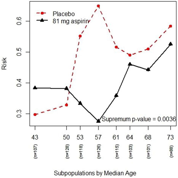
The plot shows the risk (or probability) of having adenomas (y-axis) for different age subpopulations (x-axis) for both treatment groups – the “red” dashed line is the placebo group and the “black” solid line is the 91-mg aspirin group.

Figure 2.

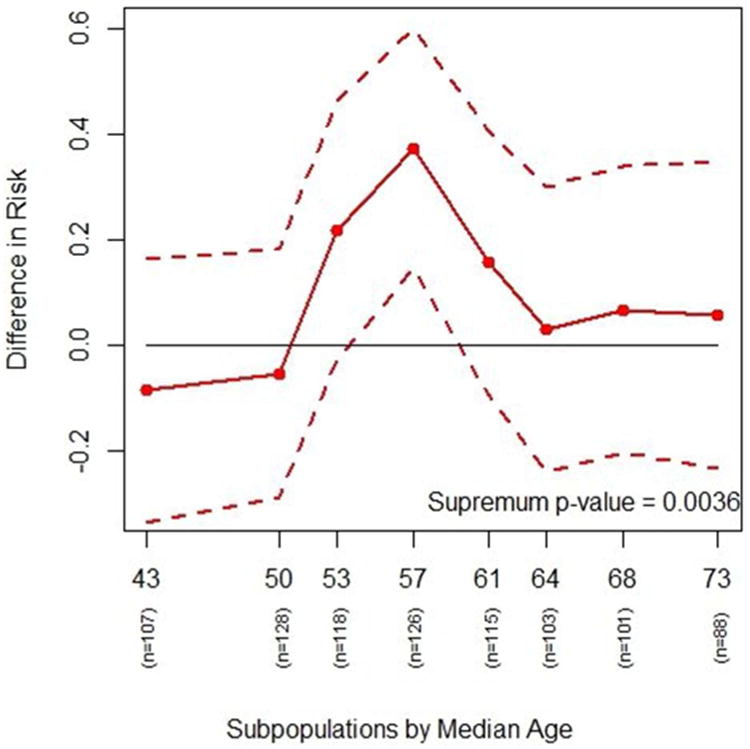
The plot shows the actual differences in risk of getting adenomas in various age subgroups between the placebo and the 81-mg aspirin treatment groups (solid line) with a 95% confidence interval (dashed lines). Differences in risk greater than zero indicate lower risk of adenomas for 81-mg aspirin compared with placebo. The interaction p-value based on risk difference is 0.0036, indicating a possible interaction effect between treatment and age. It indicates that the effect of the 81 mg to reduce the risk of having adenomas compared with placebo appears to be larger for patients in the middle age subpopulations than it is for either the youngest or oldest subpopulations.

Figure 3.

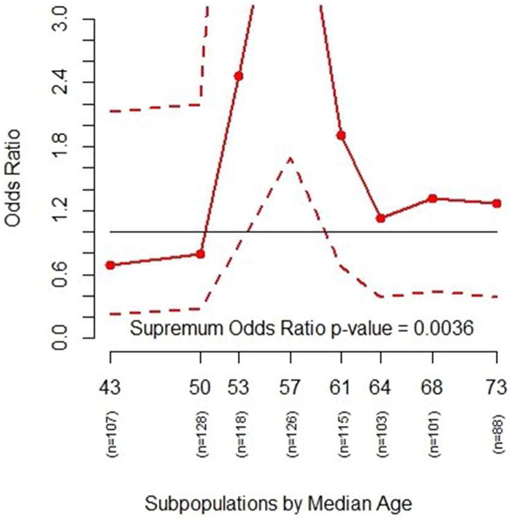
The plot shows the odds ratio of getting adenoms in various age subgroups between the placebo and the 81-mg aspirin treatment groups (solid line) with a 95% confidence interval (dashed lines). Odds ratios greater than 1.0 indicate lower risk of adenomas for 81-mg aspirin compared with placebo. The overall odds ratio of having adenomas is ∼1.46 comparing the placebo versus 81 mg of aspirin treatement groups. The interaction p-value based on odds ratio estimates is 0.0036, also indicating a possible interaction effect between treatment and age.

Note that only certain STEPP plots display the adjusted effects consistently with the model. For the Gaussian model, it would be the second plot showing the effect differences; for the Bernoulli model, it would be the third plot showing the odds ratio; and for the Poisson model, it would be the third pilot showing the relative risks. One should interpret other STEPP plots in this context cautiously.

Inference

In order to properly interpret the three STEPP plots, we associate a p-value with each of the treatment effect plots. For each subpopulation P_j, an estimate θ̂_j of treatment effect is computed. Such treatment effect estimates are clearly correlated, as there are a number of patients in common between neighboring subpopulations. For testing the absence of interaction, the following null hypothesis is of interest:

$$H_0:{\theta }_1={\theta }_2=\dots ={\theta }_K$$ (3.1)

Following the approach taken in Bonetti et al⁸ and Potthoff et al,¹⁵ we implement the permutation-based inference¹⁶ by permuting the covariate values across the patients within each treatment group and then re-computing the test statistic based on the permuted samples. The variances are also estimated from the permuted samples. The permutation p-value for a particular statistic is the proportion of the times that the permutation based statistic is more extreme than the statistic computed on the observed outcome, under the general null hypothesis of no covariate effect and no interaction.

For example, we use the following logistic model to estimate the risk: logit(p) = β₀ + β₁ * trt, where trt is the treatment indicator (0 or 1 for treatment A or B). By fitting the Bernoulli GLM to both treatment groups for each subpopulation, we can compute the difference in risk using the formula θ̂_j = p̂_A,j – p̂_B,j where p̂_G,j is the GLM estimate of the risk within treatment group G inside subpopulation P_j. The K-dimensional vector of estimates, θ̂ = (θ̂_l,…, θ̂_K), vector of overall estimates, θ̂_ALL = (θ̂_ALL,…, θ̂_ALL), and their approximate variance-covariance matrix Σ̂ are obtained via permutations.

The following test statistics can be considered to evaluate the treatment effect on the absolute scale.

1. A supremum statistic on the absolute scale:

   $$T_1={\mathit{max}}_{j=1,\dots ,K}\{|{\widehat{\theta }}_j-{\widehat{\theta }}_{\mathit{\text{ALL}}}|/\underset{{\widehat{\sigma }}_{1j}}{}\}$$ (3.2)

   where ${\widehat{\sigma }}_{1j}=\sqrt{\widehat{\mathit{\text{var}}}({\widehat{\theta }}_j-{\widehat{\theta }}_{\mathit{\text{ALL}}})}$. The supremum statistic is meant to detect sharp departures from the overall effect.

2. A quadratic form statistic on the absolute scale:

   $$T_2={(\widehat{\mathit{\theta }}-{\widehat{\mathit{\theta }}}_{\mathit{\text{ALL}}})}^T{\widehat{\sum }}^{-1}(\widehat{\mathit{\theta }}-{\widehat{\mathit{\theta }}}_{\mathit{\text{ALL}}})$$ (3.3)

   The quadratic form statistic is meant to detect global deviations from the overall effect.

3. A supremum statistic on the relative scale:

   $$T_1^{\ast }={\mathit{max}}_{j=1,\dots ,K}\{|log({\widehat{\theta }}_j)-log({\widehat{\theta }}_{\mathit{\text{ALL}}})|/\underset{{\widehat{\sigma }}_{2j}}{}\}$$ (3.5)

   where ${\widehat{\sigma }}_{2j}=\sqrt{\widehat{\mathit{\text{var}}}(log({\widehat{\theta }}_j)-log({\widehat{\theta }}_{\mathit{\text{ALL}}}))}$.

Note that examination of subpopulation treatment effect patterns may not be possible if the sample size of the trial is insufficient to support such investigation. For GLMs, if the sample size is too small there may be computational problems for estimating parameters, as the fitting algorithm may not converge. Based on our experience, at least 10 independent observations for each parameter in the model in each subpopulation seem to be a working minimum number.

One can perform a STEPP analysis with the traditional GLMs that include additional covariates besides the treatment. STEPP software uses the mean values of these additional covariates to compute the treatment effects within each subpopulation. One needs to interpret the results carefully. Adjustment for these covariates applies only to the treatment difference of the Gaussian GLM, the odds ratio of the Bernoulli GLM, and relative risks of the Poisson GLM.

For simplicity of presentation, we provide an example using Bernoulli GLM without covariates.

Results

In this section, we present the result of the simulation study under the null hypothesis of no treatment heterogeneity, a power study, and an analysis by applying the new method to the Aspirin/Folate Study dataset as an illustration.

Simulation study

We use a simulation study to evaluate the accuracy of the Type I error rate based on the statistics described in the Methods section.

Under the null hypothesis, there is no treatment effect heterogeneity across the subpopulations. We generate values for Z according to the N(25, 100) distribution for all our tests. For each of the models, the outcomes are sampled from three different distributions. Patients are randomly assigned to either treatment arm with probability 0.5.

We generate 5000 sample data sets. For each data set, we generate 4 different sample sizes. The subpopulations are constructed using different sliding window smoothing parameters.

The p-value of each data set is computed. The estimated Type I error probability is the proportion of p-values below the specified α level (which is set to 0.01, 0.05 or 0.1). The results for the Gaussian model are presented in Table 1, while the results for the other two models are provided in the Supplementary Material document. Overall, the STEPP test statistics under the null give Type I error rates that are very close to the nominal Type I error rate. In addition, we also simulate the null hypothesis when there is a treatment effect (but no treatment heterogeneity). The results are similar and provided in the Supplementary Material document.

Table 1.

Estimated Type I error probability of the permutation test for interaction based on the statistics T₁, T₂, and T₁* as defined in Section 3.2 with outcome Y under the Gaussian model N(95, 36). The distribution of the covariate of interest, Z, is N(25, 100). Results are based on 5000 simulations of sample size n, with subpopulation generating parameters r₁ and r₂.

n	r1	r2	Test Statistic	0.01	α 0.05	0.10
100	30	40	T1	0.010	0.048	0.096
			T2	0.009	0.051	0.105
			T1*	0.010	0.048	0.096
200	60	80	T1	0.010	0.052	0.101
			T2	0.009	0.053	0.106
			T1*	0.011	0.052	0.099
500	150	200	T1	0.009	0.053	0.102
			T2	0.012	0.049	0.098
			T1*	0.009	0.053	0.102
1000	300	400	T1	0.011	0.057	0.104
			T2	0.010	0.057	0.113
			T1*	0.011	0.057	0.104

Power study

For the power study, we generated 1000 datasets under three scenarios described below. Each dataset contains 500 patients, randomly assigned to either treatment arm with probability 0.5. The covariate of interest, Z, is generated from the normal distribution N(5, 2.5²). For the analysis, r₁ was set at 300 and r₂ at 400. The power of the STEPP statistics is estimated by the proportion of p-values that are smaller than the nominal significance level (α). The parameters of outcome distribution are generated using formulas based on Z, a scale factor and an offset. We considered 3 scenarios (Figure 4).

Figure 4.

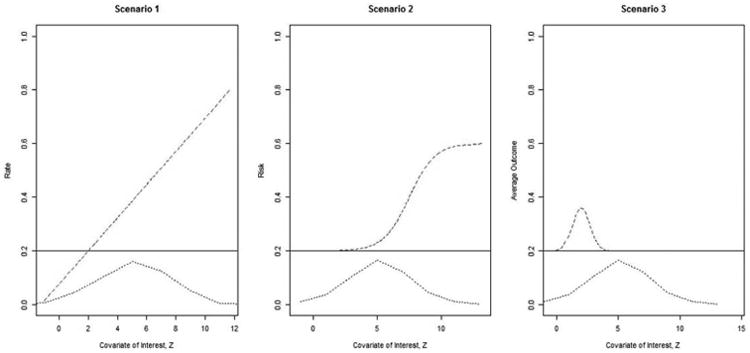
The true outcomes under the three scenarios. The bottom dashed curve is the distribution of Z. The solid line represents the hazard function of the control group (and is constant across Z); the dotted line represents the hazard function of the treatment group.

Scenario 1: The outcome of the treatment group increases linearly with Z. We use the Poisson GLM to model this scenario. Outcomes are generated using the Poisson distribution with λ = scale * z + offset.

Scenario 2: The outcome of the treatment group is the same as the control group until a given threshold is reached, after which, the risk increases quickly to a new level. We use the Bernoulli GLM to model this scenario. The baseline risk for the control group is set to 0.2 and the risk for the treatment group is set to 0.2+ scale *t/(1+t) where t = exp(z-offset). Outcomes are generated using the Bernoulli (p) distribution.

Scenario 3: The outcome of the treatment group is different for a narrow range of Z. We use the Gaussian GLM to model this scenario. The baseline mean for the control group is 0.2 and 0.2+scale* exp(-(z-offset)²) for the treatment group. Outcomes are generated using the normal distribution N(mean, 0.1²).

The results for the power at α=0.05 are presented in Table 2.

Table 2.

Estimated power of the (0.05 level) test for the statistics T₁, T₂, and T₁* as defined in Section 3.2. Sample size is 1000 with r₁=300 and r₂=400 throughout for the power study. Scale is the parameter to control the amount of deviation from null with 0 being the same as null and 0.8 the largest deviation.

		Estimated Power
Scenario	Scale	T1	T2	T1*
1	0.0	0.047	0.051	0.039
	0.1	0.105	0.090	0.055
	0.2	0.351	0.315	0.121
	0.4	0.917	0.905	0.309
	0.8	1.000	1.000	0.723
2	0.0	0.055	0.042	0.044
	0.1	0.069	0.065	0.070
	0.2	0.132	0.138	0.116
	0.4	0.447	0.478	0.335
	0.8	0.961	0.978	0.873
3	0.0	0.048	0.052	0.052
	0.1	0.070	0.069	0.069
	0.2	0.108	0.112	0.111
	0.4	0.247	0.282	0.237
	0.8	0.742	0.874	0.678

The supremum (T₁) and the chi-square (T₂) tests perform very well under all three scenarios. T₁*, which is on the relative scale, is not as powerful. It goes only to 0.73, 0.87 and 0.68, respectively.

Analysis of the Aspirin/Folate Polyp Prevention Study

The two treatment groups are placebo and 81 mg daily dosage of aspirin. We choose to model the risk, p, using logistic regression with the outcome being any occurrences of adenomas. The GLM model within each subpopulation can be written as

$$\mathit{\text{logit}}(p)={\beta }_0+{\beta }_1\ast \mathit{\text{trt}}.$$ (4.7)

The covariate of interest is age, which is treated as a continuous variable. The STEPP subpopulations are created by setting r₂ to be 100 and r₁ to be 30. Based on this setting, eight subpopulations are obtained. There are 365 patients in the placebo group and 362 patients in the 81 mg aspirin group.

Based on these eight subpopulations, treatment effect estimates of subpopulations are computed and the resulting STEPP plots are generated (Figures 1, 2, and 3). Figure 1 plots the risk of experiencing adenomas for the two treatment groups across different age subgroups. It shows that the risk for the placebo group is higher than the risk for the treatment group for age subgroups in the middle. Figure 2 plots the absolute risk difference between the two treatments across different age subgroups. Figure 3 plots the odds ratio between the two treatments across different age subgroups. The p-value of the supremum statistic is displayed in all three plots and is highly significant, indicating that sampling variability cannot account for the observed heterogeneity. As shown clearly in Figure 1, there is a trend of increasing risk of experiencing adenomas with increasing age. However, the risk of the placebo group rises quickly with age starting around age 50, while the risk for the treatment group actually decreases from the overall effect for subpopulations of patients. The two risks then come together at age 60. Indeed, the supremum statistic is good for detecting this kind of deviation.

The complete analyses are included in the Supplementary Material document. The permutation p-values when comparing placebo and the daily dosage of 325 mg of aspirin and when comparing the 81 mg and 325 mg daily aspirin dosage are not significant. Thus, the STEPP analyses confirm the original findings of the study¹² that 81mg aspirin dose reduces the risk of adenomas compared with placebo, but also highlights the age subgroup that may benefit the most from receiving low-dose aspirin.

A sensitivity analysis, constructed by varying r₂ and the ratio of r₁/r₂ is presented in the Supplementary Material document and confirms the consistency of the results.

Discussion

STEPP is a graphical tool that assists researchers in exploring the heterogeneity of treatment effects according to the value of a continuous baseline covariate across overlapping subpopulations. From the STEPP plots, one can discern treatment effect differences visually. The p-value that is shown together with each of the plots allows for an assessment of the significance of the interaction. Note that interaction depends on the scale of measurement of the treatment effect, so a careful exploration of the appropriate metric should be conducted, and the results interpreted accordingly. As STEPP allows a patient to belong to two or more overlapping subpopulations, the estimation of treatment effects borrows strength from patients in neighboring subpopulations.

The original results of the Aspirin/Folate Polyp Prevention Study data show a moderate beneficial effect on (not) experiencing adenomas with a daily dosage of 81 mg of aspirin. We applied the new methodology to the data with age as the covariate of interest. For the three comparisons, only the placebo vs. 81 mg daily aspirin dosage was statistically significant. The corresponding STEPP plot shows graphically the divergence of risk of adenomas for the two treatment groups for patients with ages approximately between 50 and 60. Thus, STEPP not only confirms the original findings, but also points to the age subgroup which may benefit the most from receiving low-dose aspirin.

Since GLM STEPP is an extension of the STEPP methodology, it has similar strengths and weaknesses. For the strengths, it is simple and flexible to use, presents good visualization of effect patterns, and provides statistical assessment of the effect patterns with good statistical properties. For the weaknesses, it cannot be used to identify exact cut points for subgroups, cannot provide multiple testing protection against different parameters and evaluating different covariate of interest. For the time-to-event data implementation of STEPP, one has to be concern with the number of events in each subpopulation. Too few events may make the estimates and the statistics unstable. In fact, we have created another type of window based on the number of events.¹⁷ GLM STEPP does not have this problem.

There are alternative approaches to assess interactions: simple regression modeling, regression splines, multivariable fractional polynomial interaction,¹⁸ Bayesian methods¹⁹ and non-parametric methods. As a comparison, we applied logistic regression, multivariable fractional polynomial interaction and the Virtual Twin²⁰ methods to the Aspirin/Folate Polyp Prevention Study data. We detected a significant interaction with age and dosage only with multivariable fractional polynomial interaction fp2 when age is categorized into 3 equal subgroups (with p-value=0.0186). The Virtual Twin method identified a similar age range, {50.5<age <59.5}, for a potential treatment effect interaction, but the treatment enhancement evaluation, Q(A), was low. The detailed results are provided in the Supplementary Material document.

STEPP is non-parametric in nature with respect to the interaction effect, and it allows one to examine possible complex interaction effects. For the sliding window, one can adjust the two window smoothing parameters to explore potential different interaction patterns. As is the case with all smoothing methods, the p-value obtained from any STEPP analysis depends upon the specific choice of the two smoothing parameter values for the sliding window approach. It is recommended that several different smoothing values be investigated in sensitivity analyses to assess the robustness of the results. For the aspirin trial example, we choose the number of patients per subpopulation (r₂) to be 100 and the largest number of patients in common between two consecutive subpopulations (r₁) to be 30. This choice generated 8 subpopulations providing a good view of the treatment effects along age for analysis. Based on our experience and supported by the sensitivity analyses shown in the Supplementary Material document, the following are general guidelines for choosing r₁ and r₂: (1) Choose r₂ large enough to obtain a good estimate of the treatment effect within subpopulations; (2) Create at least 4-5 subpopulations; (3) Choose r₁/r₂ to be about 30-50% as your initial investigation; (4) Make r₁, r₂ larger to obtain a smoother STEPP plot, but not so large that you have less than 4 subpopulations; (5) To assess the consistency of the result, a sensitivity analysis varying r₂ is recommended.

The current STEPP software has some limitations. It is restricted to continuous, binary and count data modeled by standard GLMs. It restricts the analysis to the comparison of two treatment groups. Further, it allows for the study of only one covariate of interest. Note that one may use as the covariate of interest a baseline composite risk score, which can be a function of several baseline characteristics, as done in Viale et al.¹⁰

The Type I error rates are close to the nominal rate. Although the power study only considers a limited number of alternative scenarios, it shows that the test statistics have good power to detect differences, both on the absolute and relative scales. In general, one still needs to adjust for multiple testing if several different covariates are evaluated one at a time. In addition, the approach does not address the fact that one is performing post-hoc analyses.

It should be noted that STEPP is an exploratory tool. In particular, it is not meant to be used to determine specific cut-points in the range of values of the covariate of interest, but rather to provide some indication regarding the ranges of values where the new treatment might be particularly beneficial (or detrimental). Future research work is needed to investigate how to use STEPP to identify cut-points based on cross validation studies.²¹ The permutation p-value indicating the statistical significance of the observed heterogeneity should always be presented together with the graphical presentation of STEPP to avoid over-interpretation of the graphical results. Also, results should be confirmed using results from other data sets investigating similar treatment comparisons.

Supplementary Material

Table A: Comparing 81 mg of aspirin with placebo. When the ratio r₁/r₂ >= 50%, most of the test statistics become significant. Also, tests are more significant when there are more subpopulations. The highlighted row was used for the aspirin study analysis in the manuscript.

Table B: Comparing 81 mg of aspirin with 325 mg of aspirin. None of the test statistics is significant for any combination of r₁ and r₂.

Table C: Comparing 325 mg of aspirin with placebo. A small number of tests are borderline significant especially when r₁/r₂ is above 70%.

References

- 1.Lagakos SW. The challenge of subgroup analysis – Reporting without distorting. N Engl J Med. 2006;354:1667–1669. doi: 10.1056/NEJMp068070. [DOI] [PubMed] [Google Scholar]
- 2.Wang R, Lagakos SW, Ware JH, et al. Statistics in medicine – Reporting of subgroup analyses in clinical trials. N Engl J Med. 2007;357:2189–2194. doi: 10.1056/NEJMsr077003. [DOI] [PubMed] [Google Scholar]
- 3.Cox DR. Regression models and life tables (with discussion) J R Stat Soc Series B Stat Methodol. 1972;34:187–220. [Google Scholar]
- 4.Fine J, Gray R. A proportional hazards model for the sub distribution of a competing risk. J Am Stat Assoc. 1999;94:496–509. [Google Scholar]
- 5.Gray R. A class of k-sample tests for comparing the cumulative incidence of a competing risk. Ann Stat. 1998;16:1141–1154. [Google Scholar]
- 6.Bonetti M, Gelber RD. A graphical method to assess treatment-covariate interactions using the cox model on subsets of the data. Stat Med. 2000;19:2595–2609. doi: 10.1002/1097-0258(20001015)19:19<2595::aid-sim562>3.0.co;2-m. [DOI] [PubMed] [Google Scholar]
- 7.Bonetti M, Gelber RD. Patterns of treatment effects in subsets of patients in clinical trials. Biostatistics. 2004;53:465–481. doi: 10.1093/biostatistics/5.3.465. [DOI] [PubMed] [Google Scholar]
- 8.Bonetti M, Zahrieh D, Cole D, et al. A small sample study of the stepp approach to assessing treatment-covariate interactions in survival data. Stat Med. 2009;28:1255–1268. doi: 10.1002/sim.3524. [DOI] [PMC free article] [PubMed] [Google Scholar]
- 9.Lazar A, Cole B, Bonetti M, et al. Evaluation of treatment-effect heterogeneity using biomarkers measured on a continuous scale: Subpopulation treatment effect pattern plot. J Clin Oncol. 2010;28:4539–4544. doi: 10.1200/JCO.2009.27.9182. [DOI] [PMC free article] [PubMed] [Google Scholar]
- 10.Viale G, Giobbie-Hurder A, Regan MM, et al. Prognostic and predictive value of centrally reviewed ki-67 labeling index in postmenopausal women with endocrine-responsive breast cancer: Results from breast international group trial 1-98 comparing adjuvant tamoxifen with letrozole. J Clin Oncol. 2008;26:5569–5575. doi: 10.1200/JCO.2008.17.0829. [DOI] [PMC free article] [PubMed] [Google Scholar]
- 11.Colleoni M, Litman HJ, Castiglione-Gertsch M, et al. Duration of adjuvant chemotherapy for breast cancer: a joint analysis of two randomized trials investigating three versus six course of cmf. Br J Cancer. 2002;86:1705–1714. doi: 10.1038/sj.bjc.6600334. [DOI] [PMC free article] [PubMed] [Google Scholar]
- 12.Baron JA, Cole BF, Sandler RS, et al. A randomized trial of aspirin to prevent colorectal adenomas. N Engl J Med. 2003;348:891–899. doi: 10.1056/NEJMoa021735. [DOI] [PubMed] [Google Scholar]
- 13.R Foundation for Statistical Computing, Austria. Vienna: 2008. R: A language and environment for statistical computing. http://CRAN.R-project.org. [Google Scholar]
- 14.Yip WK. stepp: Subpopulation Treatment Effect Pattern Plot (STEPP): R package version 2.3-2. 2011 http://CRAN.R-project.org/package=stepp.
- 15.Potthoff RF, Peterson BL, George SL. Detecting treatment-by-centre interaction in multi-centre clinical trials. Stat Med. 2001;20:193–213. doi: 10.1002/1097-0258(20010130)20:2<193::aid-sim651>3.0.co;2-#. [DOI] [PubMed] [Google Scholar]
- 16.Pesarin F. Multivariate permutation tests: with application in Biostatistics. 1st. New York: Wiley; 2001. [Google Scholar]
- 17.Lazar AA, Bonetti M, Cole BF, et al. Identifying treatment effect heterogeneity in clinical trials using subpopulations of events: STEPP. Clin Trials. 2015 Oct 22; doi: 10.1177/1740774515609106. Epub ahead of print. [DOI] [PMC free article] [PubMed] [Google Scholar]
- 18.Royston P, Sauerbrei W. A new approach to modeling interaction between treatment and continuous covariates in clinical trials by using fractional polynomials. Stat Med. 2004;23:2509–2525. doi: 10.1002/sim.1815. [DOI] [PubMed] [Google Scholar]
- 19.Simon R. Bayesian subset analysis: Application to studying treatment-by-gender interactions. Stat Med. 2002;21:2909–29016. doi: 10.1002/sim.1295. [DOI] [PubMed] [Google Scholar]
- 20.Foster JC, Taylor JMG, Rubert SJ. Subgroup identification from randomized clinical trial data. Stat Med. 2011;30:2867–2880. doi: 10.1002/sim.4322. [DOI] [PMC free article] [PubMed] [Google Scholar]
- 21.Pogue-Geile KL, Kim C, Jeong JH, et al. Predicting degree of benefit from adjuvant trastuzumab in nsabp trial b-31. J Natl Cancer Inst. 2013;105:1782–1788. doi: 10.1093/jnci/djt321. [DOI] [PMC free article] [PubMed] [Google Scholar]
Associated Data
This section collects any data citations, data availability statements, or supplementary materials included in this article.
Supplementary Materials