A Comparison of Lung Nodule Segmentation Algorithms: Methods and Results from a Multi-institutional Study

Abstract

Tumor volume estimation, as well as accurate and reproducible borders segmentation in medical images, are important in the diagnosis, staging, and assessment of response to cancer therapy. The goal of this study was to demonstrate the feasibility of a multi-institutional effort to assess the repeatability and reproducibility of nodule borders and volume estimate bias of computerized segmentation algorithms in CT images of lung cancer, and to provide results from such a study. The dataset used for this evaluation consisted of 52 tumors in 41 CT volumes (40 patient datasets and 1 dataset containing scans of 12 phantom nodules of known volume) from five collections available in The Cancer Imaging Archive. Three academic institutions developing lung nodule segmentation algorithms submitted results for three repeat runs for each of the nodules. We compared the performance of lung nodule segmentation algorithms by assessing several measurements of spatial overlap and volume measurement. Nodule sizes varied from 29 μl to 66 ml and demonstrated a diversity of shapes. Agreement in spatial overlap of segmentations was significantly higher for multiple runs of the same algorithm than between segmentations generated by different algorithms (p < 0.05) and was significantly higher on the phantom dataset compared to the other datasets (p < 0.05). Algorithms differed significantly in the bias of the measured volumes of the phantom nodules (p < 0.05) underscoring the need for assessing performance on clinical data in addition to phantoms. Algorithms that most accurately estimated nodule volumes were not the most repeatable, emphasizing the need to evaluate both their accuracy and precision. There were considerable differences between algorithms, especially in a subset of heterogeneous nodules, underscoring the recommendation that the same software be used at all time points in longitudinal studies.

Introduction

Globally, lung cancer is the leading cause of cancer-related deaths in males and the second leading cause of cancer-related deaths in females [1]. Imaging plays a key role in patient care during all stages of the disease including diagnosis, staging, management, and assessing response to therapy [2, 3]. More recently, a number of trials [4] including the National Lung Screening Trial (NLST) [5] have provided compelling evidence that in some populations, the mortality associated with lung cancer can be reduced by screening using low-dose CT (LDCT) [6], thus adding screening to the list of imaging roles.

When pulmonary nodules are identified on CT scans, criteria developed by the Fleischner Society [7] and others call for a follow-up scan in 3–12 months to assess its growth rate. Tumor doubling time has been proposed as a marker for malignancy [8–10], and the current standard for measuring tumor response, Response Evaluation Criteria in Solid Tumors (RECIST) [11], is based on uni-dimensional, linear measurements of tumor diameter. Measurements are made manually, and significant inter-observer variability exists [12–14]. For response assessment, as well as diagnosis and staging, there is considerable interest in developing accurate and precise segmentations of lung tumors, which can in turn provide both linear and volumetric assessments of tumor size and change rates. Indeed, The Nederlands Leuvens Longkanker Screenings Onderzoek (NELSON) trial, the largest European lung cancer screening trial, uses volumetric measurements and volume doubling times (VDT) as criteria for assessing the risk of malignancy. Although automatic and semi-automatic segmentation algorithms can facilitate these tasks, analysis of three software packages using data from the NELSON study indicated that they “yield significant differences in volumetric measurements and VDT” and that “this variation affects the classification of lung nodules” [15]. It has also been reported that, in nodules detected during screening, three segmentation algorithms within the same software package could not be used interchangeably, as different algorithms delivered significantly different volumes [16].

Various commercial entities offer systems for lung tumor size determination, and new ones are introduced periodically. While accuracy of lung nodule segmentation can only be assessed in phantoms, it is important to be able to assess reproducibility under changes in operator input and inter-algorithm agreement in human-subject datasets from an appropriate cohort.

In this study, we conducted a lung nodule “segmentation challenge” among three academic institutions with an interest in developing segmentation algorithms and evaluated their repeatability, reproducibility, and bias utilizing a previously developed software platform [17–19] that facilitates comparison of segmentation algorithms.

Materials and Methods

Datasets

All image data used in this study were collected by the respective institutions following approval by their respective Institutional Review Boards and de-identified for HIPAA compliance. These datasets were then deposited in The Cancer Imaging Archive (TCIA: http://cancerimagingarchive.net/) and are available to the public through a shared list for easy download [20]. They consisted of 52 tumors in 41 CT volumes from 5 sub-collections: (A) one CT study of a phantom containing 12 synthetic nodules scanned at Columbia University Medical Center (CUMC) [21], (B) 10 CT studies selected from the publicly available Lung Imaging Database Consortium (LIDC) [22–24], (C) 10 CT studies from the Reference Image Database to Evaluate Response (RIDER) [21] to therapy in cancer collections, (D) 10 CT studies from Moffitt Cancer Center (MCC), and (E) 10 CT studies from Stanford University (SU) [25]. Table 1 contains demographic and key scanning parameters for all the sub-collections.

Table 1.

Demographics and selected scanner parameters for the five collections used in our study

Collection	Scanned at site	No. (males, females)	Mean age (range)	kVp	mA range	Slice thickness range (mm)	Number of slices per study range	Acquisition year (range)
A	CUMC	N/A (phantom)	N/A (phantom)	120	195	1.25	237	2011
B	LIDC	10 (gender not available)	not available	120	80–360	1.0–2.5	166–481	Not available
C	RIDER	10 (genders unknown)	58 (44–71)	120	Auto (238–439)	1.25	47–186	2006–2007
D	MCC	10 (4, 6)	67.7 (49, 78)	120	(280–545)	3	103–150	2000–2009
E	SU	10 (7, 3)	65.4 (46, 80)	120	Auto (123–751)	0.625–1.25	69–307	2008–2010

While all 41 CT volumes have been used in prior studies [21–23, 25–27], they have never been used as a set for the comparison of segmentation algorithms, as we present here, and there therefore is no scientific overlap between the work described here and prior publications.

Algorithms

Three academic institutions developing lung nodule segmentation algorithms submitted results for three repeat runs on each nodule. Thus, data from a total of 3 × 3 × 52 = 468 segmentations were analyzed for this study. These segmentations have also been deposited in TCIA and are available to the public through a shared list [20]. The following is a brief description of each algorithm used.

Algorithm 1

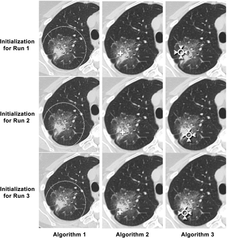
This algorithm is based on the image processing techniques of marker-controlled watershed, geometric active contours and Markov random field [28]. It requires manual initialization of a region of interest (ROI) that encloses the lesion on a single image, as seen in Fig. 1. Then the entire tumor volume can be automatically obtained. In this study, two additional segmentation runs were initiated by randomly changing the long axis, the short axis, and the central point of the ellipsoid ROI drawn in the first run. The allowed range for the two axes and the center’s x and y coordinates was 10 % of either the long or short axis.

Fig. 1.

Example initializations for each of the runs for each algorithm for one of the nodules

Algorithm 2

A single click ensemble segmentation (SCES) algorithm using a proprietary platform [27] was used for lung nodule segmentation as seen in Fig. 1. In brief, the algorithm is based on using multiple seed points with region growing. It makes use of the “Click and Grow” algorithm by using a manually selected initial seed point to define an area, within which multiple seed points are automatically generated. Ensemble segmentation can be obtained from the multiple regions that were grown. In this algorithm, ensemble segmentation refers to a set of different input segmentations (multiple runs using same segmentation technique but different initializations) that are combined in order to generate consensus segmentation. Repeat runs started with an independently selected seed point.

Algorithm 3

This algorithm begins with a completely automated lung segmentation, which establishes a 3D boundary beyond which tumors cannot exist. This lung segmentation algorithm employs a smoothness constraint so that tumors in contact with the chest wall and/or mediastinum are not falsely excluded from the lung field, although large tumors may be problematic. However, this was not a problem in the dataset used for this study. A manually placed seed “circle” supplied location and gray-value statistics that were used to initialize the nodule segmentation algorithm as seen in Fig. 1. Two-dimensional region growing was then initiated starting at the centroid of the seed circle using thresholds computed from the gray values in the seed circle. Gray-value statistics were then updated based on the region grown, and the points included in the grown region were then projected into the adjacent superior and inferior sections and used as seeds for region growing in those sections using thresholds computed from the updated statistics. This proceeded iteratively until points projected into adjacent sections were outside of the computed thresholds. In all sections, morphological operations prevented growth into attached blood vessels, and growth beyond the computed lung segmentation boundary was not allowed. Repeat runs started with independently placed seed circles on different though representative sections and positioned to include solid and ground-glass components if the nodules were part-solid.

Imaging informatics platform

We extended a previously developed imaging informatics platform [17–19] for the task of evaluating segmentations in the context of a lung nodule segmentation challenge. The platform was already capable of the following:

1. Automated quantitative inter-observer and intra-observer volume of interest (VOI) analyses and comparisons

2. A collection of pilot data to develop and validate quality metrics for institutional and cooperative group quality assurance efforts

We extended this platform to support a number of additional formats for the lung nodule segmentation challenge including Portable Network Graphics (PNG), Annotation and Image Markup (AIM) [29], and DICOM Segmentation Object (DSO) [30] as these were the formats generated by the three software tools being evaluated. Converters were written to convert all formats into common formats in order to be able to compare segmentations generated by the various algorithms.

The platform has analytical and statistical libraries to calculate a number of commonly used metrics to support segmentation evaluations, as described below and in Table 2.

Table 2.

Statistical measures used in this study

Metric	Definition	References
Volume	Number of voxels in object multiplied by the voxel size in mm3
Bias	An estimate of systematic measurement error; it is the difference between the mean of measurements made on the same object and the measurement’s true value. Percent bias is bias divided by the true value times 100 %.	Kessler [21]
Dice coefficient	(Volume of the intersection of regions A and B divided by the volume of their union)	Dice [30]
Repeatability/reproducibility	“Precision under a set of repeatability (reproducibility) conditions of measurement”	Raunig [20]
		Kessler [21]
Precision	“Closeness of agreement between measured quantity values obtained by replicate measurements on the same or similar experimental units under specified conditions”; can be estimated using wSD, wCV, RC, ICC, CCC (see below)	Raunig [20]
		Kessler [21]
		Barnhart [26]
Within-subject standard deviation (wSD)	σ	Kessler [21]
Within-subject coefficient of variation (wCV)	σ/μ	Obuchowski (19 )
Repeatability coefficient (RC)	“The least significant difference between two repeated measurements on a case taken under the same conditions”	Kessler [21]
		Obuchowski [19]
		Bland [27]
Intra-class correlation coefficient (ICC)	Consistency of repeated measures relative to the total variability in the population (assumes independent normally distributed samples)	Raunig [20]
		Shrout [24]
Concordance correlation coefficient (CCC)	Consistency of repeated measures relative to the total variability in the population	Lin [23]

Statistical Analyses and Metrics

The goal of this study was to evaluate the performance of the algorithms in terms of their bias, repeatability, and reproducibility [31–33] as well as to obtain insights into the underlying reasons for differences between algorithms on a voxel level.

Bias

The bias of the volume measurement was calculated for the nodules for which the ground truth was available (the 12 nodules in the phantom dataset) as the difference between estimated and true volume. As described [31–33], we estimated the population bias utilizing a repeated measures analysis to estimate the sample mean difference. Proportional bias was computed as the bias divided by the true value [31–33]. Two-way ANOVA (algorithm, nodule) was used to test the null hypothesis that there is no difference in bias between algorithms.

Volume repeatability was measured based on the computed volumes of repeat segmentations provided by a given algorithm for each nodule. This was performed considering all 52 nodules. Commonly used measures for repeatability include the repeatability coefficient (RC), the within-subject coefficient of variation (wCV), and the concordance correlation coefficient (CCC) [31–33]. The RC is defined as:

$$RC=1.96\sqrt{2{\mathrm{\sigma }}_{\in }^2}=2.77{\mathrm{\sigma }}_{\in }$$

where σ²_∈ is the within-subject variance.This RC is understood as “the least significant difference between two repeated measurements taken under identical conditions at a two-sided significance of α  = 0.05” [32].

The wCV is defined as:

$$wCV\mathit{=}\frac{{\sigma }_{\in }}{\mu }$$

where μ is the mean of the volume measurements. The CCC [34, 35] has been proposed to address some deficiencies of the intra-class correlation coefficient (ICC) [36], another commonly used measure [36–38]. ICC requires the assumptions of ANOVA while CCC does not. However, when normality is assumed, the CCC equals the ICC [34, 36, 37]. Although we report the CCC here, this measure does suffer from notable deficiencies common to many of these correlation measures [39–41] in that they are very sensitive to sample heterogeneity and that they are aggregate measures (thus making it difficult to separate systematic bias from issues in precision or large random errors). Thus, it would not be valid to compare our CCC measures to those measured on a different set of nodules with a different range of volumes.

Volume reproducibility was measured based on the computed volumes of segmentations provided by all three algorithms for each nodule, using the reproducibility coefficient RDC (analogous to RC [32, 33]), wCV, and CCC as defined above for repeatability.

Spatial Overlap

Dice scores [42] were used to estimate the spatial overlap between segmentations within algorithms (i.e., pairwise comparisons between repeat segmentations provided by each algorithm) and between algorithms (all pairwise comparisons between segmentations provided by different algorithms). A novel use of intra-algorithm Dice scores is as measures of repeatability and reproducibility. This metric would detect differences between segmentations having the same volume but different locations/surfaces. Dice scores are not normally distributed as they have an upper bound of 1 and are typically skewed left. We used non-parametric statistics for the comparison of Dice scores.

Table 2 summarizes the metrics used in this study. For more details, readers are referred to a series of papers published on statistical methods for quantitative imaging biomarkers [31–33, 41].

Results

Datasets

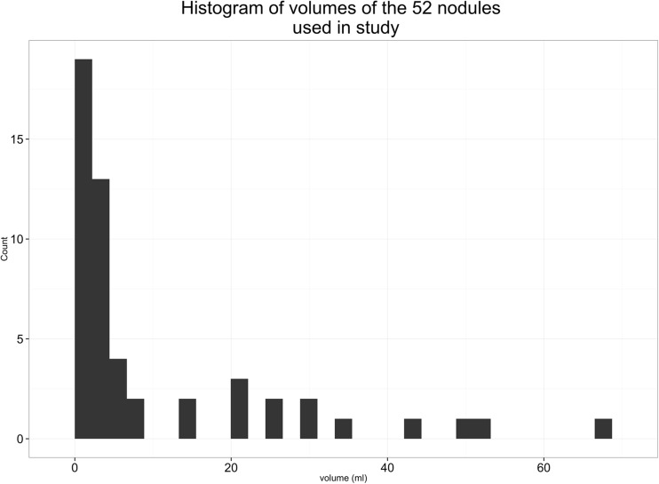
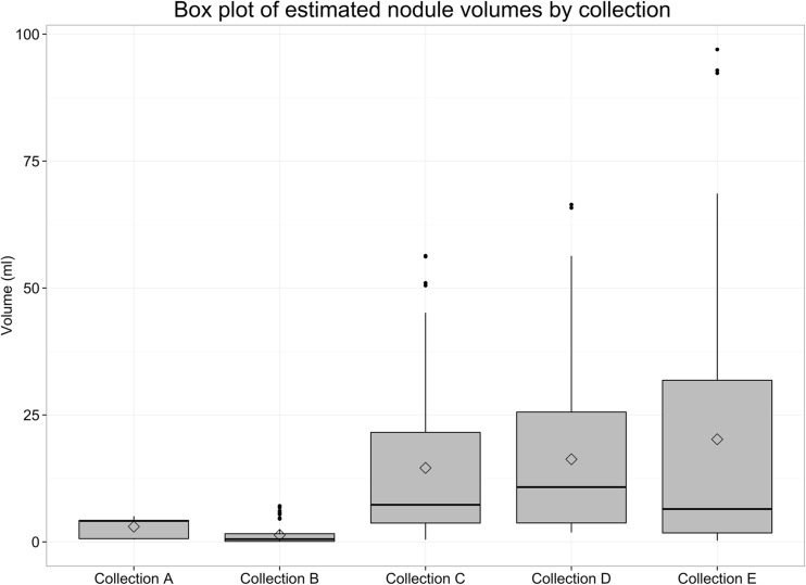
The image data used for this study, consisting of CT scans of 52 lesions, demonstrated large diversity in the size and shape of the nodules. Figure 2 shows the distribution of the estimated nodule sizes of all 468 segmentation; the median of volume measurements for each nodule over all three runs of three segmentation algorithms varied over three orders of magnitude from 0.029 to 66.53 ml. Figure 3 shows that the phantom data (collection A) and LIDC (collection B) typically had smaller nodules (p < 0.05) compared to collections C, D, and E while collection E had the largest variation in nodule sizes.

Fig. 2.

Distribution of nodule sizes as estimated by the median over all segmentations for each nodule

Fig. 3.

Box plot of nodule volumes by collection displays the range of nodule sizes

Bias in estimated volumes

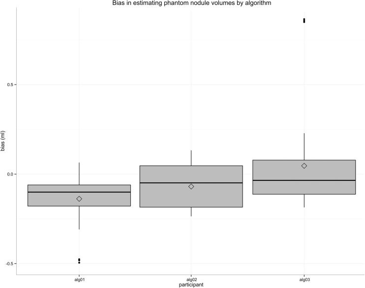
Figure 4 plots the bias in the volume estimate for the phantom nodules compared to known truth and shows that algorithm 3 has the least negative bias while algorithm 1 has the most. ANOVA revealed a statistically significant difference in bias between algorithms, with the mean bias for algorithms 1, 2, and 3 being −0.138, −0.069, and 0.046 ml, respectively (p < 0.05).

Fig. 4.

Volume measurement bias by algorithm demonstrating that algorithm 3 has the least negative bias while algorithm 1 has the most

Additionally, Table 3 shows the results of a post hoc comparison using the Tukey HSD method [43], indicating that pairwise differences in bias between algorithms 1 and 3 and 2 and 3 are significant while the difference between algorithms 1 and 2 is not significant. When comparing the proportional biases, algorithm 2 had the least negative bias while algorithm 1 had the most negative bias. However, only the difference in proportional bias between algorithms 1 and 2 was significant.

Table 3.

Pairwise differences in bias and proportional bias between algorithms on phantom nodules

Bias Comparison	Difference (ml) (95% confidence interval)	p Value
Alg 2 vs alg 1	0.068 (−0.010–0.147)	0.097
Alg 3 vs alg 1	0.184 (0.106–0.263)	0.0000006
Alg 3 vs alg 2	0.116 (0.037–0.194)	0.0019782
Proportional bias comparison	Difference (%) (95 % confidence interval)	p Value
Alg 2 vs alg 1	0.079 (0.027–0.131)	0.0013742
Alg 3 vs alg 1	0.045 (−0.007–0.097)	0.1066724
Alg 3 vs alg 2	−0.034 (−0.086–0.018)	0.2667675

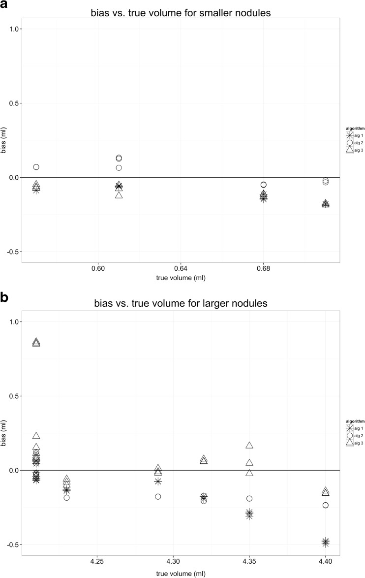
The 12 nodules in this collection can be grouped into two size categories: small (0.57–0.71 ml) and large (4.21–4.4 ml). Figure 5 suggests that the patterns of bias for the algorithms appear to be different for the large nodules compared to the smaller nodules. Algorithm 3 has negative bias for smaller nodules and generally positive bias for larger nodules while the pattern is flipped for algorithm 2. Algorithm 1 tends to have a negative bias for all nodule sizes.

Fig. 5.

Volume measurement bias in a small and b large nodules suggests that the patterns of bias for the algorithms are different for the large nodules compared to the smaller nodules

Spatial Overlap Between Segmentations as a Function of Collection

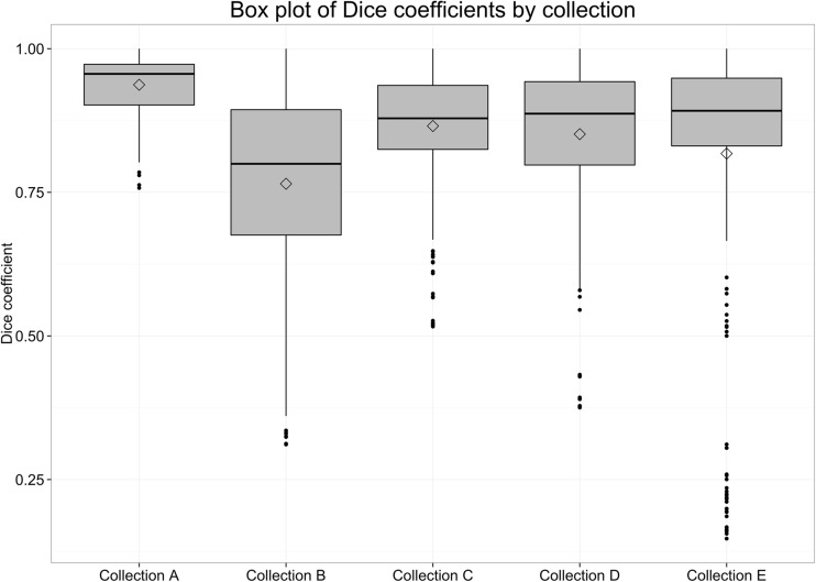
Figure 6 compares the distribution of all pairwise Dice scores for the different collections. This allows us to explore if there are differences in agreement between algorithms as a function of the collection. The Kruskal-Wallis non-parametric ANOVA, used because the Dice scores were not normally distributed and had unequal variances, indicated that the phantom nodules (collection A) had statistically significantly higher agreement between segmentations produced by the different algorithms compared to the other collections (p < .05). Post hoc tests, adjusting for multiple comparisons, further indicated that there was no significant difference in agreement among algorithms between the three diagnostic collections (C–E) (p < .05), while the LIDC collection (collection B) had the least agreement between algorithms and the difference was significant (p < .05). The LIDC (collection B) was from a screening trial and had the smallest nodules (as seen in Fig. 3). Thus, even small variations in the segmentations generated by the algorithms can result in lower Dice scores. In fact, previous studies with human expert annotators and the LIDC dataset had already demonstrated the lack of consensus in locating and segmenting nodules in this collection [24].

Fig. 6.

Distribution of Dice scores by collection highlighting better agreement between segmentations on phantom data (collection A) compared to clinical data (collections B–E)

Repeatability and Reproducibility

The upper section of Table 4 shows the results of our volume repeatability (i.e., the agreement over multiple initializations of a given algorithm over all samples) analysis by the traditional measures of wCV, RC, and the CCC. Algorithm 2 was the most repeatable while algorithm 3 was the least, but, in all cases, the estimate of wCV was less than 10 %. As was discussed earlier, although the CCCs are very high for all three algorithms, this is primarily an artifact of the heterogeneity of the samples (large range of tumor volumes) and not really a good measure of the repeatability of the algorithms.

Table 4.

Repeatability and reproducibility of algorithmic determination of nodule volume

Repeatability
Algorithm	RC (ml)	wCV	CCC (95 % confidence interval)
Alg 1	1.830	6.29 %	0.997 (0.981–0.999)
Alg 2	1.266	4.64 %	0.999 (0.995–0.999)
Alg 3	2.626	7.92 %	0.996 (0.970–0.999)
Reproducibility
Nodules	RDC (ml)	wCV	CCC (95 % confidence interval)
52	10.34	36.65 %	0.836 (0.752–0.893)

RC repeatability coefficient, RDC reproducibility coefficient, wCV within-subject coefficient of variation, CCC concordance correlation coefficient

The lower section of Table 4 shows results of our volume reproducibility (i.e., the agreement of all of the algorithms over all samples) using the same measures as above (but with RC replaced by the RDC). Not surprisingly, the CCC, which in this analysis considered all nine results per nodule (three each from three algorithms), was considerably lower than results from the repeatability analysis, which considered each algorithm separately. This was also true for RC (vs RDC) and wCV.

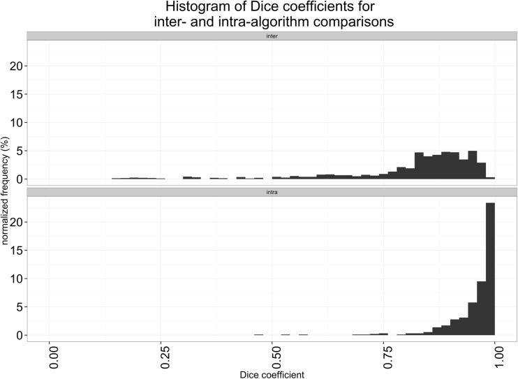
For each nodule, we also calculated all pairwise Dice scores for all nine segmentations available for that nodule. We grouped these into intra-algorithm (i.e., repeatability) and inter-algorithm (i.e., reproducibility) sets. Figure 7 shows the distribution of the pairwise Dice scores for each nodule. As is expected, there is greater spatial overlap between multiple runs of a single algorithm than between algorithms. The intra-algorithm agreement (repeatability) was significantly higher than the inter-algorithm agreement (reproducibility); the average Dice score was 0.95 versus 0.81 (p < 0.001; Wilcoxon rank sum test) and was typically higher for larger volumes, though this was not statistically significant.

Fig. 7.

Histograms of Dice scores of (top) inter- and (bottom) intra-algorithm pairwise comparisons. Intra-algorithm Dice scores are significantly higher than inter-algorithm Dice scores indicating better robustness to user initializations than to choice of algorithm

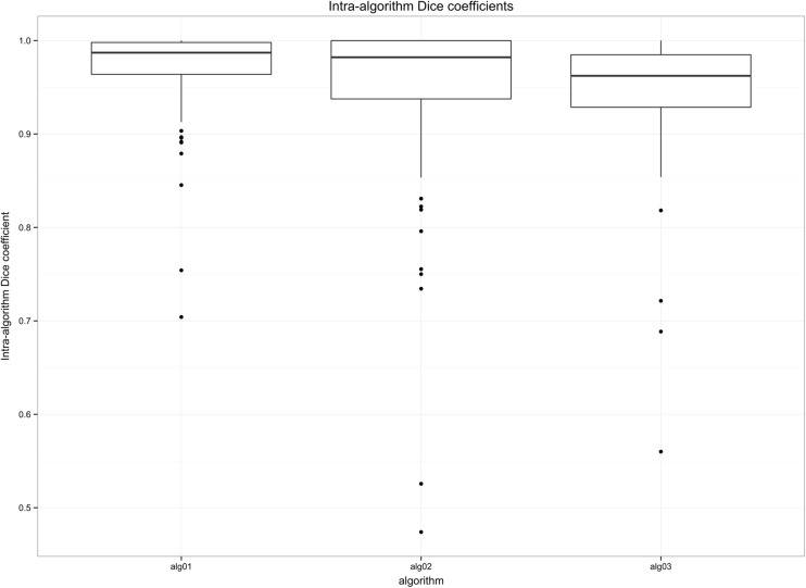
Figure 8 demonstrates the intra-algorithm distribution of Dice scores, a measure of the repeatability of the algorithms. The Kruskal-Wallis multiple comparison test [44] indicated that algorithms 1 and 2 had significantly higher Dice scores than algorithm 3 (p < .05), suggesting their higher repeatability.

Fig. 8.

Box plot comparing intra-algorithm Dice coefficients between algorithms, demonstrating that algorithms 1 and 2 were more repeatable than algorithm 3

Exploring Causes of Variability

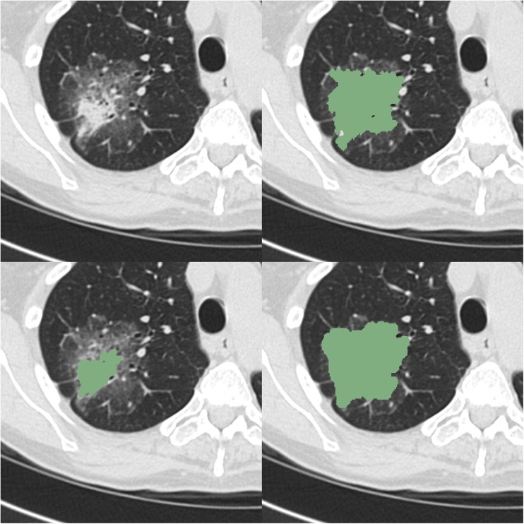
In order to further understand the underlying causes of variability between the segmentations produced by the different algorithms, we studied the Dice coefficients by nodule for all nodules in collection E, which had a range of Dice coefficients. We could immediately see that two nodules have high variability. We then compared the estimated volumes for the different algorithms for the nodule with the highest variability and observed very large differences in estimated volumes between segmentations produced by the three algorithms. Visualizing segmentations from each algorithm for this nodule (Fig. 9) allows us to see the nodule that results in the difference in boundaries generated by the algorithms.

Fig. 9.

Variability in the results of three segmentation algorithms for a nodule with low inter-algorithm Dice coefficients illustrated on a single cross-section

Discussion

This study evaluated the repeatability and reproducibility of semi-automatic segmentation algorithms developed at three academic institutions on 52 lung nodules in lung CT scans from five different collections of images. We were able to demonstrate statistically significant differences in bias as well as repeatability and reproducibility between the algorithms and to explore some of the reasons for these differences.

The repeatability of algorithms, measured both using Dice scores between segmentations generated by the same algorithms and the concordance of volumes estimated by these segmentations, was significantly higher than the reproducibility (inter-algorithm comparisons). This underscores the recommendation that the same software be used at all time points in longitudinal studies and in measurement of parameters such as tumor doubling time.

We found better agreement between the segmentations generated for the algorithms on the phantom data compared to the clinical scans, highlighting the need for evaluating the performance of algorithms on clinical data in addition to phantoms. In addition, the agreement was quite poor on the screening data (collection B, LIDC), suggesting the need for continuing development of algorithms for use with the smaller nodules typically seen in screening settings.

Limitations and Conclusions

This study was primarily aimed at demonstrating the feasibility of a performing multi-institutional algorithm comparison study, specifically of segmentation algorithms, using an informatics platform developed for the purpose. Because we used a small number of nodules, we cannot draw conclusions about the relative performance of the algorithms tested. However, we have demonstrated a general paradigm and precise methods for comparing segmentations of medical images and for exploring the sources of variability and their manifestations. Despite the fact that we limited our study to segmentations of lung nodules in CT scans, these methods are perfectly generalizable to any modality generating 2D images or 3D volumes and can be easily adapted for assessments of nodule growth over time.

References

- 1.Torre LA, Bray F, Siegel RL, Ferlay J, Lortet-Tieulent J, Jemal A. Global cancer statistics, 2012. CA Cancer J Clin. 2015;65(2):87–108. doi: 10.3322/caac.21262. [DOI] [PubMed] [Google Scholar]
- 2.Ravenel JG. Evidence-based imaging in lung cancer: a systematic review. J Thorac Imaging. 2012;27(5):315–324. doi: 10.1097/RTI.0b013e318254a198. [DOI] [PubMed] [Google Scholar]
- 3.Rivera MP, Mehta AC, Wahidi MM. Establishing the diagnosis of lung cancer: Diagnosis and management of lung cancer, 3rd ed: American College of Chest Physicians evidence-based clinical practice guidelines. Chest. 2013;143(5 Suppl):e142S–e165S. doi: 10.1378/chest.12-2353. [DOI] [PubMed] [Google Scholar]
- 4.Nair A, Hansell DM. European and North American lung cancer screening experience and implications for pulmonary nodule management. Eur Radiol. 2011;21(12):2445–2454. doi: 10.1007/s00330-011-2219-y. [DOI] [PubMed] [Google Scholar]
- 5.National Lung Screening Trial Research Team. Aberle DR, Adams AM, Berg CD, Black WC, Clapp JD, Fagerstrom RM, Gareen IF, Gatsonis C, Marcus PM, Sicks JD. Reduced lung-cancer mortality with low-dose computed tomographic screening. N Engl J Med. 2011;365(5):395–409. doi: 10.1056/NEJMoa1102873. [DOI] [PMC free article] [PubMed] [Google Scholar]
- 6.National Lung Screening Trial Research Team. Church TR, Black WC, Aberle DR, Berg CD, Clingan KL, Duan F, Fagerstrom RM, Gareen IF, Gierada DS, Jones GC, Mahon I, Marcus PM, Sicks JD, Jain A, Baum S. Results of initial low-dose computed tomographic screening for lung cancer. N Engl J Med. 2013;368(21):1980–1991. doi: 10.1056/NEJMoa1209120. [DOI] [PMC free article] [PubMed] [Google Scholar]
- 7.MacMahon H, Austin JH, Gamsu G, Herold CJ, Jett JR, Naidich DP, Patz EF, Jr, Swensen SJ, Fleischner S. Guidelines for management of small pulmonary nodules detected on CT scans: a statement from the Fleischner Society. Radiology. 2005;237(2):395–400. doi: 10.1148/radiol.2372041887. [DOI] [PubMed] [Google Scholar]
- 8.Revel MP. Avoiding overdiagnosis in lung cancer screening: the volume doubling time strategy. Eur Respir J. 2013;42(6):1459–1463. doi: 10.1183/09031936.00157713. [DOI] [PubMed] [Google Scholar]
- 9.Patel VK, Naik SK, Naidich DP, Travis WD, Weingarten JA, Lazzaro R, Gutterman DD, Wentowski C, Grosu HB, Raoof S. A practical algorithmic approach to the diagnosis and management of solitary pulmonary nodules: part 2: pretest probability and algorithm. Chest. 2013;143(3):840–846. doi: 10.1378/chest.12-1487. [DOI] [PubMed] [Google Scholar]
- 10.Infante M, Berghmans T, Heuvelmans MA, Hillerdal G, Oudkerk M. Slow-growing lung cancer as an emerging entity: from screening to clinical management. Eur Respir J. 2013;42(6):1706–1722. doi: 10.1183/09031936.00186212. [DOI] [PubMed] [Google Scholar]
- 11.Eisenhauer EA, Therasse P, Bogaerts J, Schwartz LH, Sargent D, Ford R, Dancey J, Arbuck S, Gwyther S, Mooney M, Rubinstein L, Shankar L, Dodd L, Kaplan R, Lacombe D, Verweij J: New response evaluation criteria in solid tumours: Revised RECIST guideline (version 1.1). 45(2):228–247, 2009. doi:10.1016/j.ejca.2008.10.026 [DOI] [PubMed]
- 12.Revel MP, Bissery A, Bienvenu M, Aycard L, Lefort C, Frija G. Are two-dimensional CT measurements of small noncalcified pulmonary nodules reliable? Radiology. 2004;231(2):453–458. doi: 10.1148/radiol.2312030167. [DOI] [PubMed] [Google Scholar]
- 13.Reeves AP, Biancardi AM, Apanasovich TV, Meyer CR, MacMahon H, van Beek EJ, Kazerooni EA, Yankelevitz D, McNitt-Gray MF, McLennan G, Armato SG, 3rd, Henschke CI, Aberle DR, Croft BY, Clarke LP. The Lung Image Database Consortium (LIDC): a comparison of different size metrics for pulmonary nodule measurements. Acad Radiol. 2007;14(12):1475–1485. doi: 10.1016/j.acra.2007.09.005. [DOI] [PMC free article] [PubMed] [Google Scholar]
- 14.Marten K, Auer F, Schmidt S, Kohl G, Rummeny EJ: Inadequacy of manual measurements compared to automated CT volumetry in assessment of treatment response of pulmonary metastases using RECIST criteria - Springer. European. 2006 [DOI] [PubMed]
- 15.Zhao YR, Ooijen PMv, Dorrius MD, Heuvelmans M, de Bock GH, Vliegenthart R, Oudkerk M: Comparison of three software systems for semi-automatic volumetry of pulmonary nodules on baseline and follow-up CT examinations. Acta radiologica (Stockholm, Sweden : 1987). 2013. doi:10.1177/0284185113508177 [DOI] [PubMed]
- 16.Ashraf H, de Hoop B, Shaker SB, Dirksen A, Bach KS, Hansen H, Prokop M, Pedersen JH. Lung nodule volumetry: segmentation algorithms within the same software package cannot be used interchangeably. Eur Radiol. 2010;20(8):1878–1885. doi: 10.1007/s00330-010-1749-z. [DOI] [PMC free article] [PubMed] [Google Scholar]
- 17.Kalpathy-Cramer J, Fuller CD: Target Contour Testing/Instructional Computer Software (TaCTICS): a novel training and evaluation platform for radiotherapy target delineation.2010:361–365, 2010 [PMC free article] [PubMed]
- 18.Kalpathy-Cramer J, Bedrick SD, Boccia K, Fuller CD: A pilot prospective feasibility study of organ-at-risk definition using Target Contour Testing/Instructional Computer Software (TaCTICS), a training and evaluation platform for radiotherapy target delineation.2011:654–663,2011 [PMC free article] [PubMed]
- 19.Kalpathy-Cramer J, Awan M, Bedrick S, Rasch CR, Rosenthal DI, Fuller CD. Development of a software for quantitative evaluation radiotherapy target and organ-at-risk segmentation comparison. J Digit Imaging. 2014;27(1):108–119. doi: 10.1007/s10278-013-9633-4. [DOI] [PMC free article] [PubMed] [Google Scholar]
- 20.Kalpathy-Cramer J, Napel S, Goldgof D, Zhao B: QIN multi-site collection of Lung CT data with Nodule Segmentations https://wiki.cancerimagingarchive.net/display/DOI/QIN+multi-site+collection+of+Lung+CT+data+with+Nodule+Segmentations2015 [cited 2015]. Available from: doi:10.7937/K9/TCIA.2015.1BUVFJR7
- 21.Zhao B, James LP, Moskowitz CS, Guo P, Ginsberg MS, Lefkowitz RA, Qin Y, Riely GJ, Kris MG, Schwartz LH. Evaluating variability in tumor measurements from same-day repeat CT scans of patients with non-small cell lung cancer. Radiology. 2009;252(1):263–272. doi: 10.1148/radiol.2522081593. [DOI] [PMC free article] [PubMed] [Google Scholar]
- 22.Clarke LP, Croft BY, Staab E, Baker H, Sullivan DC. National Cancer Institute initiative: Lung image database resource for imaging research. Acad Radiol. 2001;8(5):447–450. doi: 10.1016/S1076-6332(03)80555-X. [DOI] [PubMed] [Google Scholar]
- 23.Turner WD, Kelliher TP, Ross JC, Miller JV. An analysis of early studies released by the Lung Imaging Database Consortium (LIDC) Med Image Comput Comput Assist Interv. 2006;9(Pt 2):487–494. doi: 10.1007/11866763_60. [DOI] [PubMed] [Google Scholar]
- 24.Armato SG, III, McNitt-Gray MF, Reeves AP, Meyer CR, McLennan G, Aberle DR, Kazerooni EA, MacMahon H, van Beek EJ, Yankelevitz D, Hoffman EA, Henschke CI, Roberts RY, Brown MS, Engelmann RM, Pais RC, Piker CW, Qing D, Kocherginsky M, Croft BY, Clarke LP. The Lung Image Database Consortium (LIDC): an evaluation of radiologist variability in the identification of lung nodules on CT scans. Acad Radiol. 2007;14(11):1409–1421. doi: 10.1016/j.acra.2007.07.008. [DOI] [PMC free article] [PubMed] [Google Scholar]
- 25.Gevaert O, Xu J, Hoang CD, Leung AN, Xu Y, Quon A, Rubin DL, Napel S, Plevritis SK. Non-small cell lung cancer: identifying prognostic imaging biomarkers by leveraging public gene expression microarray data—methods and preliminary results. Radiology. 2012;264(2):387–396. doi: 10.1148/radiol.12111607. [DOI] [PMC free article] [PubMed] [Google Scholar]
- 26.Zhao B, Tan Y, Tsai WY, Schwartz LH, Lu L. Exploring variability in CT characterization of tumors: a preliminary phantom study. Transl Oncol. 2014;7(1):88–93. doi: 10.1593/tlo.13865. [DOI] [PMC free article] [PubMed] [Google Scholar]
- 27.Gu Y, Kumar V, Hall LO, Goldgof DB, Li C-Y, Korn R, Bendtsen C, Velazquez ER, Dekker A, Aerts H, Lambin P, Li X, Tian J, Gatenby RA, Gillies RJ. Automated delineation of lung tumors from CT images using a single click ensemble segmentation approach. Pattern Recogn. 2013;46(3):692–702. doi: 10.1016/j.patcog.2012.10.005. [DOI] [PMC free article] [PubMed] [Google Scholar]
- 28.Tan Y, Schwartz LH, Zhao B. Segmentation of lung lesions on CT scans using watershed, active contours, and Markov random field. Med Phys. 2013;40(4):043502. doi: 10.1118/1.4793409. [DOI] [PMC free article] [PubMed] [Google Scholar]
- 29.Channin DS, Mongkolwat P, Kleper V, Sepukar K, Rubin DL. The caBIG annotation and image Markup project. J Digit Imaging. 2010;23(2):217–225. doi: 10.1007/s10278-009-9193-9. [DOI] [PMC free article] [PubMed] [Google Scholar]
- 30.Dicom Standards Committee WG. Digital Imaging and Communications in Medicine (DICOM) Supplement 111 [cited 2014]. Available from: ftp://medical.nema.org/medical/dicom/final/sup111_ft.pdf
- 31.Obuchowski NA, Reeves AP, Huang EP, Wang XF, Buckler AJ, Kim HJ, Barnhart HX, Jackson EF, Giger ML, Pennello G, Toledano AY, Kalpathy-Cramer J, Apanasovich TV, Kinahan PE, Myers KJ, Goldgof DB, Barboriak DP, Gillies RJ, Schwartz LH, Sullivan AD: Quantitative imaging biomarkers: A review of statistical methods for computer algorithm comparisons. Statistical methods in medical research. 2014. doi:10.1177/0962280214537390 [DOI] [PMC free article] [PubMed]
- 32.Raunig DL, McShane LM, Pennello G, Gatsonis C, Carson PL, Voyvodic JT, Wahl RL, Kurland BF, Schwarz AJ, Gonen M, Zahlmann G, Kondratovich M, O’Donnell K, Petrick N, Cole PE, Garra B, Sullivan DC, Group QTPW: Quantitative imaging biomarkers: A review of statistical methods for technical performance assessment. Statistical methods in medical research. 2014. doi:10.1177/0962280214537344 [DOI] [PMC free article] [PubMed]
- 33.Kessler LG, Barnhart HX, Buckler AJ, Choudhury KR, Kondratovich MV, Toledano A, Guimaraes AR, Filice R, Zhang Z, Sullivan DC, Group QTW The emerging science of quantitative imaging biomarkers terminology and definitions for scientific studies and regulatory submissions. Stat Methods Med Res. 2014 doi: 10.1177/0962280214537333. [DOI] [PubMed] [Google Scholar]
- 34.Barnhart HX, Haber M, Song J. Overall concordance correlation coefficient for evaluating agreement among multiple observers. Biometrics. 2002;58(4):1020–1027. doi: 10.1111/j.0006-341X.2002.01020.x. [DOI] [PubMed] [Google Scholar]
- 35.Lin LI. A concordance correlation coefficient to evaluate reproducibility. Biometrics. 1989;45(1):255–268. doi: 10.2307/2532051. [DOI] [PubMed] [Google Scholar]
- 36.Shrout PE, Fleiss JL. Intraclass correlations: uses in assessing rater reliability. Psychol Bull. 1979;86(2):420–428. doi: 10.1037/0033-2909.86.2.420. [DOI] [PubMed] [Google Scholar]
- 37.Barnhart HX, Haber MJ, Lin LI: An overview on assessing agreement with continuous measurements. 17(4):529–569, 2007. doi:10.1080/10543400701376480 [DOI] [PubMed]
- 38.Barnhart HX, Barboriak DP. Applications of the repeatability of quantitative imaging biomarkers: a review of statistical analysis of repeat data sets. Transl Oncol. 2009;2(4):231–235. doi: 10.1593/tlo.09268. [DOI] [PMC free article] [PubMed] [Google Scholar]
- 39.Bland JM, Altman DG. Statistical methods for assessing agreement between two methods of clinical measurement. Lancet. 1986;1(8476):307–310. doi: 10.1016/S0140-6736(86)90837-8. [DOI] [PubMed] [Google Scholar]
- 40.Nevill AM, Atkinson G. Assessing agreement between measurements recorded on a ratio scale in sports medicine and sports science. Br J Sports Med. 1997;31(4):314–318. doi: 10.1136/bjsm.31.4.314. [DOI] [PMC free article] [PubMed] [Google Scholar]
- 41.Obuchowski NA, Barnhart HX, Buckler AJ, Pennello G, Wang XF, Kalpathy-Cramer J, Kim HJ, Reeves AP, for the Case Example Working G Statistical issues in the comparison of quantitative imaging biomarker algorithms using pulmonary nodule volume as an example. Statistical methods in medical research. Stat Methods Med Res. 2015;24(1):107–140. doi: 10.1177/0962280214537392. [DOI] [PMC free article] [PubMed] [Google Scholar]
- 42.Dice LR. Measures of the amount of ecologic association between species. Ecology. 1945;26(3):297–302. doi: 10.2307/1932409. [DOI] [Google Scholar]
- 43.Tukey J. Comparing individual means in the analysis of variance. Biometrics. 1949;5(2):99–114. doi: 10.2307/3001913. [DOI] [PubMed] [Google Scholar]
- 44.Siegel S, Castellan NJ., Jr . Nonparametric Statistics for the Behavioral Sciences. 2. New York: McGraw-Hill Humanities/Social Sciences/Languages; 1988. [Google Scholar]