Coherent stochastic oscillations enhance signal detection in spiking neurons

Abstract

We study the effect of noisy oscillatory input on the signal discrimination by spontaneously firing neurons. Using analytically tractable model, we contrast signal detection in two situations (i) when the neuron is driven by coherent oscillations and (ii) when the coherence of oscillations is destroyed. Analytical calculations revealed a region in the parameter space of the model, where oscillations act to reduce the variability of neuronal firing and to enhance the discriminability of weak signals. These analytical results are employed to unveil a possible role of coherent oscillations in peripheral electrosensory system of paddlefish in improvement of detection of weak stimuli. The proposed mechanism may be relevant to a wide range of phenomena involving coherently driven oscillators.

I. INTRODUCTION

Rhythmic activity is observed at all levels of nervous systems [1]. Recently, neuronal oscillations have been shown to improve the stimulus discrimination, either by increasing the precision of spike timing [2] or by inducing binomial statistics of serially binned spike counts across a neuronal population [3]. Here, we explore a different mechanism of discrimination enhancement, whereby coherent stochastic oscillations driving a periodically spiking neuron induce long-lasting serial correlations of interspike intervals (ISIs) that suppress variability of spike counts. This situation is encountered, for example, by a CNS neuron receiving coherent oscillatory inputs in gamma band, or in a “hair cell – afferent” sensory receptors for hearing, balance, and electrosense.

The significance of anticorrelated ISIs in shaping neuronal responses was experimentally demonstrated in electroreceptors of a weakly electric fish [4, 5], where negative correlations of sequential ISIs originate from intrinsic properties of sensory neurons. Theoretical studies have shown that a negative feedback mechanism either in a network [6] or in a single neuron with a dynamic threshold [7, 8] can induce anticorrelations of sequential ISIs, which reduce long-time variability and thereby lead to enhanced information transfer of low frequency stimuli. In this scenario, the correlations structure is fixed by the negative feedback parameters.

The long lasting ISI anticorrelations can also result from the interaction of unidirectionally coupled noisy oscillators, as was shown in peripheral electroreceptors of paddlefish [9]. In this system, noisy oscillations in sensory epithelia drive sensory neurons and act as an internal narrow-band noise, that leads to reduced low-frequency fluctuations of neuronal firing [17, 18]. The structure and extent of serial ISI correlations in this feed-forward scenario are set by the frequency and coherence of driving oscillations. This could potentially provide an active adjustment mechanism to achieve enhanced discrimination on behaviorally relevant time scales.

The structure of ISI correlations in the neuron driven by slow, exponentially correlated noise was also explored by several analytical studies using integrate and fire models [13, 14, 16]. It was found that exponentially correlated noise leads to positive serial ISI correlations, which enhance variability of neuronal firing at long time scales. The Fano factor, a measure of spike count variability on different time scales, shows a minimum, indicating an optimal time scale at which variability of spike counts is lowest and hence the detection of weak signals is optimal [13].

Here, we aim to analyze how the signal detection depends on the correlations structure, as well as to contrast the signal detection by a spiking neuron driven by either coherent stochastic oscillations or by fluctuations whose coherence is destroyed. In both latter cases, the neuron firing is constrained to have identical first order ISI statistics, but it lacks any ISI correlations if the oscillations coherence is destroyed. Using an analytically tractable model we calculate the parameter region where coherent stochastic oscillations enhance signal detection. The analytical model predictions are then verified using the experimental data from paddlefish electroreceptors [9].

II. METHODS AND MODEL

A. Spike count variability and discriminability

To assess the performance of a spontaneously firing neuron as a detector for weak signals s, we apply the ideal observer paradigm [10] to the neuron’s output spike train y(t) = Σ_iδ(t − t_i), where {t_i} is the sequence of spike times. The observable is the spike count $n(T)={\int }_t^{t+T}y(t^{\prime })d{t}^{\prime }$ in a parameter-fixed time window T. Decision about the presence of a constant signal s is made on the basis of comparing spike count distributions P_s(n, T) and P₀(n, T) in two situations: when a neuron is stimulated or spontaneously firing, respectively. The separation of the two distributions, is characterized by the discriminability measure

$$d^{\prime }=2[\mid {\mu }_s(T)-{\mu }_0(T)\mid ]/[{\sigma }_s(T)+{\sigma }_0(T)],$$ (1)

where μ and σ are the mean and the standard deviation of the spike count, respectively. The variability of the spike count is assessed by the Fano factor [10],

$$F(T)={\sigma }^2(T)/\mu (T).$$ (2)

We assume that for a weak stimuli, σ(T) is not affected by the signal, and the Fano factor Eq. 2 and the discriminability Eq. 1 are related as

$$d^{\prime }=\alpha \sqrt{{\mu }_0(T)/F_0(T)},$$ (3)

where α is the relative change in the mean firing rate due to stimulus [7]. Eq. 3 establishes the relation between spontaneous spike count variability and discriminability of weak signals: smaller Fano factor, i.e. smaller variability of the spike count of spontaneous firing, results in larger discriminability. The dependence of the discriminability d′ on the signal strength α is linear with the slope $\sqrt{{\mu }_0(T)/F_0(T)}$.

Variability of the spike count depends on the correlation structure of the spike train. The correlations can be quantified by the serial correlation coefficients ρ_k = (〈I_iI_i+k〉 − 〈I〉²)/var(I) between interspike intervals, I_i = t_i − t_i−1. The asymptotic value of the Fano factor F (T) is determined, if the serial correlation coefficients (SCCs) are summed over all lags: ${lim}_{T\to \infty }F(T)={CV}^2(1+2{\sum }_{k=1}^{\infty }{\rho }_k)$, where $CV=\sqrt{var(I)}/\langle I\rangle$ is the coefficient of variation [11]. On intermediate time scales, the variability of the spike count depends crucially on the correlations structure, with positive ISI correlations acting to increase, while negative ISI correlations acting to suppress spike count variability [7, 12]. In the case of renewal spiking, when sequential ISIs are uncorrelated, ρ_k = δ_0,k, the Fano factor approaches CV² for large T.

B. Model

Previous study [17] showed that long lasting serial correlations is a generic result of an unidirectional coupling of two noisy oscillators. Here we aim to study how the signal detection performance of a neuron depends on the temporal structure of ISI correlations, and to contrast the signal detection by a neuron with long lasting serial ISI correlations versus a neuron lacking serial ISI correlations, when both neurons have identical first order ISIs statistics. We employ two analytically tractable models, which we refer to as renewal and nonrenewal. These models differ in the coherence of driving noise, but otherwise have identical ISI distributions and linear response properties. In both models, periodic spiking is mimicked by a perfect integrate-and-fire (PIF) model as in Refs. [13, 14]. It is driven by two statistically independent Gaussian noises: a narrow-band noise y(t), representing coherent stochastic oscillations, and an exponentially correlated noise η(t), mimicking slow fluctuations [13]:

$$\begin{array}{ll}\stackrel{.}{x}& =\lambda +y+\eta ,\\ \stackrel{.}{y}& =z,\stackrel{.}{z}=-\gamma z-{\omega }_0^{2}y+A{\omega }_0\sqrt{2\gamma }{\xi }_1(t).\\ \stackrel{.}{\eta }& =-\eta /{\tau }_c+{\sigma }_{\eta }\sqrt{2/{\tau }_c}{\xi }_2(t).\end{array}$$ (4)

The first equation for x in Eqs. 4 is the perfect integrator. Whenever x(t) reaches the threshold x_b = 1, a spike is generated and x immediately resets to the initial value x_r = 0. The parameter λ sets the mean firing rate of the model, f_a = λ. A constant stimulus is modeled as a change in the parameter λ. The two equations for y and z model narrow-band noise with the peak spectrum frequency $f_e=(1/2\pi )\sqrt{{\omega }_0^2-{\gamma }^2/4}$ and the variance A². The coherence of the narrow-band noise is measured by the quality factor Q = 2πf_e/γ. Finally, the last equation describes the Ornstein-Uhlenbeck (OU) noise η(t) with the correlation time τ_c and the variance ${\sigma }_{\eta }^2$. The OU noise is slow relative to the average period of spiking, τ_c ≫ 1/λ, and is introduced to account for slow fluctuations observed in sensory neurons [7]. The terms ξ_1,2(t) are statistically independent Gaussian white noise sources with unit intensity.

For convenience, we introduce a vector r(t) = {y(t), z(t), η(t)} for the three dimensional Gaussian process driving the perfect integrator. In the nonrenewal model, the noise vector r(t) evolves independently of spiking dynamics according to Eqs. 4. In the renewal model, all components of the noise vector are reset at every spiking to a new value r₀ = {y₀, z₀, η₀} randomly sampled from the noise upon firing distribution ℘(r₀). This is the stationary distribution of r values at the instants of firing in the nonrenewal model. In both models, the values of noise variables at the beginning of each ISI are drawn from the same distribution. Consequently the ISI densities are identical for both models. However, the renewal model exhibits no ISI correlations, since the noise values at the beginning of each ISI are sampled from the distribution ℘(r₀) at random, i.e. independently of the duration of the previous ISI, and of the noise value at the instants of firing.

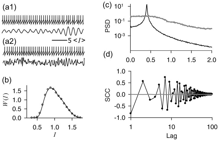
Figure 1 shows numerical simulations of the models. Although the firing patterns (Fig. 1a) of both renewal and nonrenewal models look very similar and the ISI densities are identical (Fig. 1b), their SCCs (Fig. 1d) are significantly different. This difference appears because the coherence of narrow-band noise y(t) is destroyed in the renewal model as demonstrated in Fig. 1c, where the power spectra of driving noise y(t) in both models are depicted.

FIG. 1.

Numerical simulation of the model Eqs. 4. (a): Time series of the “voltage” variable x (upper trace) and noise y(t) (lower trace) for the nonrenewal (a1) and renewal (a2) models. (b): Probability density of ISIs, W (I) for renewal (solid line) and nonrenewal (open circles) models. (c): Power spectral densities (PSD) of noise y(t) in renewal (grey line) and nonrenewal (black line) models. (d): Serial correlation coefficients (SCC) of spike trains produced by renewal (grey line) and nonrenewal (black line with circles) models. The parameters are λ = 2, A² = 0.2, f_e/f_a = 0.4, Q = 20.0, τ_c = 375, σ_η = 0.5 · 10⁻⁴, f_e/f_a = 0.43. Time axes are in units of mean interspike intervals. The frequency axis in panel (c) is scaled by the mean firing rate f_a = 2.

C. Analytical calculation of the Fano factor

Our goal is to contrast the discriminability in the renewal and nonrenewal models Eqs. 4, and to analyze the discriminability in the nonrenewal model as a function of the coherence and frequency of the driving oscillations. To this end, we calculate analytically the Fano factor of the spike trains. Since the dependence of the discriminability d′ on the signal strength α is linear (Eq. 3), the relative performance of the renewal and nonrenewal models can be characterized by the ratio R(T) of their discriminability slopes:

$$R(T)=\sqrt{\frac{{\mu }_n(T)}{F_n(T)}}\sqrt{\frac{F_r(T)}{{\mu }_r(T)}}.$$ (5)

The values of R(T) > 1 indicate that the signal detection performance is better in the nonrenewal than in the renewal model.

Calculations of statistical properties of the spike train are largely simplified if N consecutive ISIs are replaced by a passage from x_r to sequentially x_b, 2x_b … kx_b … and Nx_b [14]. Since the right hand sides in Eqs. 4 do not explicitly depend on x, this is possible if recrossing of a threshold is highly unprobable, i.e. if the noise intensity is small relative to the drift term λ:

$$A^2+{\sigma }_{\eta }^2\ll {\lambda }^2/2.$$ (6)

Assume, we start our observation at time t = 0, when the value of the voltage variable is x₀. The voltage value x₀ + x at time T is determined by the transition probability density P_x(x₀ + x, T |x₀, 0) = P_x(x, T |0, 0) for the x-variable:

$$P_x(x,T\mid 0,0)=\int d\mathbf{r}d{\mathbf{r}}_{0}P(x,\mathbf{r},T\mid 0,{\mathbf{r}}_0,0)P_{st}({\mathbf{r}}_0).$$ (7)

Here P (x, r, T |x₀, r₀, t₀) is the transition probability density for the multidimensional Gaussian process given by Eqs. 4 without reset, and P_st(r₀) is the stationary probability density of the noise variables. These probability densities are readily obtained analytically [21].

The number of spike-counts N_T within the time-window T is equal to the number of “thresholds” nx_b contained within the interval (x₀, x₀ + x), see Fig. 2. For nx_b < x < (n + 1)x_b, it holds

FIG. 2.

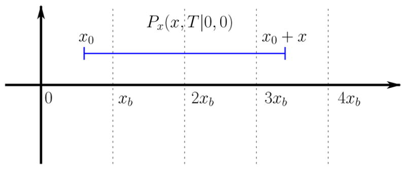
Illustration to the calculation of the Fano factor.

$$N_T=\{\begin{array}{ll}n+1\hfill & \text{with}\text{probability}\frac{x-n{x}_b}{x_b},\hfill \\ n\hfill & \text{with}\text{probability}\frac{(n+1)x_b-x}{x_b},\hfill \end{array}$$ (8)

since the initial position x₀ is uniformly distributed along the x-axis.

According to Eq. 8, the mean of the spike-count 〈N_nx〉 for a fixed value of x ∈ (nx_b, (n + 1)x_b) is calculated as

$$\begin{array}{l}\langle N_{nx}\rangle =(n+1)\frac{x-n{x}_b}{x_b}+n\frac{(n+1)x_b-x}{x_b}\\ =x/x_b.\end{array}$$ (9)

Analogously, the mean square of the spike-count 〈 $N_{nx}^2$〉 for a fixed value of x ∈ (nx_b, (n+1)x_b) equals

$$\langle N_{nx}^2\rangle =(2n+1)\frac{x}{x_b}-n(n+1).$$

To obtain the mean μ_o(T) and the variance ${\sigma }_o^2(T)$ of the spike count, we average 〈N_nx〉 and 〈 $N_{nx}^2$〉 over all values of x:

$$\begin{array}{l}{\mu }_o(T)=\sum _{n=0}^{\infty }{\int }_{n{x}_b}^{(n+1)x_b}\langle N_{nx}\rangle P_x(x,T\mid 0,0)dx,\\ {\sigma }_o^2(T)=\sum _{n=0}^{\infty }{\int }_{n{x}_b}^{(n+1)x_b}\langle N_{nx}^2\rangle P_x(x,T\mid 0,0)dx-{\mu }_o^2(T).\end{array}$$ (10)

This leads to the following expressions for the mean and the variance of the spike count:

$$\begin{array}{l}{\mu }_o(T)=\frac{1}{x_b}{\int }_0^{\infty }x{P}_x(x,T\mid 0,0)dx,\\ {\sigma }_o^2(T)=\sum _{k=0}^{\infty }\left[\frac{2k+1}{x_b}{\int }_{k{x}_b}^{(k+1)x_b}x{P}_x(x,T\mid 0,0)dx-k(k+1){\int }_{k{x}_b}^{(k+1)x_b}{P}_x(x,T\mid 0,0)dx\right]-{\mu }_o^2(T).\end{array}$$ (11)

The integrals in Eqs. 11 are evaluated analytically, and the infinite sum is approximated numerically.

For the renewal model, the mean of the spike count equals μ_r (T) = Tλ, and its variance is expressed as [10]

$${\sigma }_r^2(T)=T\lambda +2T{\int }_0^T\left(1-\frac{\tau }{T}\right){\rho }^{+}(\tau )d\tau ,$$ (12)

where ρ⁺(τ) = ρ(τ) − λδ(τ) with ρ(τ) being the autocorrelation function of the renewal spike train [15]:

$${\rho }^{+}(\tau )=\frac{\lambda }{2\pi }{\int }_{-\infty }^{\infty }{e}^{-i\omega \tau }\frac{1-{\mid \widehat{W}(\omega )\mid }^2}{{\mid 1-\widehat{W}(\omega )\mid }^2}d\omega -\lambda \delta (\tau ).$$ (13)

Here, Ŵ(ω) = 〈e^iωI〉 is the Fourier transform of the ISI density W (I). For weak noise, when recrossing of the threshold is very unprobable, the ISI density can be approximated by the Rice density of level-crossings [14, 19, 20]:

$$W(I)=\int d\mathbf{r}d{\mathbf{r}}_0(\lambda +y+\eta )P(x_b,\mathbf{r},I\mid x_r,{\mathbf{r}}_0,0)\mathcal{P}({\mathbf{r}}_0).$$ (14)

Here ℘(r₀) is related to the stationary density P_st(r₀) of the Gaussian noise via ℘(r₀) = [(λ+y₀ + η₀)/λ]P_st(r₀) [11]. The integrals in Eq. 14 extend over the phase space region where ẋ = μ + η + y > 0. For weak noise intensities (see Eq. 6), it holds that (λ + y₀ + η₀)/λ ≈ 1 everywhere in the phase space, where P_st(r₀) is significantly different from zero. Therefore, without loss of accuracy, we approximate the noise upon firing density ℘(r₀) in Eq. 14 by the stationary density P_st(r₀) and extend the integration limits to the whole phase space. The integrals in Eq. 14 are then evaluated analytically, and then the Fano factor is calculated numerically using Eqs. 12,13 and the fast Fourier transform.

III. RESULTS AND DISCUSSION

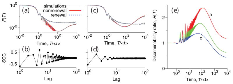
The dependence of the Fano factor and SCCs on the coherence of oscillations is illustrated in Fig. 3a–d for the nonrenewal (solid red lines) and renewal (dotted blue lines) models. The theoretical Fano curves perfectly overlap with the results of numerical simulations (grey lines). For intermediate time scales 10〈I〉 < T < 200〈I〉, the Fano factor of the nonrenewal model, F_n(T), becomes strikingly smaller than that of the renewal model, F_r(T), and exhibits a minimum at T ≈ 200〈I〉. F_n(T) increases for T > 200〈I〉, due to slow fluctuations leading to positive ISI correlations [13, 16], while F_r(T) saturates to its theoretical limit of CV².

FIG. 3.

(Color online) (a),(c): Analytical Fano factor curves for renewal (dotted blue lines) and nonrenewal (solid red lines) models. For both models, the results of numerical simulations are shown as grey solid lines. (b),(d): numerically calculated SCCs ρ_k. The parameters are λ = 2, A² = 0.2; (a),(b): f_e/f_a = 0.4, Q = 20.0, τ_c = 375, σ_η = 0.5 · 10⁻⁴; (c),(d): f_e/f_a = 0.5, Q = 4.0, τ_c = 900, σ_η = 1.5 · 10⁻⁴. (e): Ratio of discriminability slopes in the nonrenewal and renewal models for parameter sets as in panels (a),(c) (red and blue lines, respectively), and for f_e/f_a = 0.47, Q = 10.0, τ = 600, σ_η = 10⁻⁴ (green line).

As expected, changes in Q almost do not influence the spike count variability in the renewal model, but do have a strong impact on the variability in the nonrenewal model. With higher values of Q, corresponding to more coherent oscillations (Fig. 3a,b, Q = 20), serial correlations extend up to hundreds of ISIs, the minimum in the Fano factor of the nonrenewal model is deep, and the reduction in the spike-count variability relative to the renewal model can reach up to one order of magnitude, on time scales between 10 and 1000 〈I〉. A decreased coherence of oscillations, reflected in lower Q values, results in brief ISI correlations, a shallower minimum in the Fano factor of the nonrenewal model, and a smaller reduction in variability relative to the renewal model (Fig. 3c,d, Q = 4). The suppression of the spike count variability due to oscillations translates to the enhancement of the discriminability, which is characterized by the discriminability ratio R(T) (Eq. 5) shown in Fig. 3e. The maximal value of R(T) decreases with decreasing oscillation coherence.

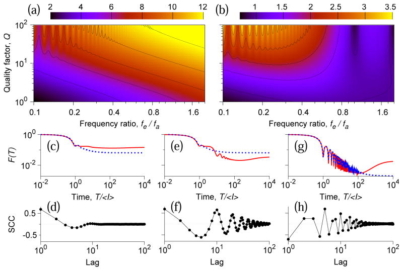
Fig. 4 summarizes the dependence of discriminability on the oscillation to firing frequency ratio f_e/f_a, and the quality factor Q. If f_e is low (small f_e/f_a), then several ISIs occur during one oscillation cycle, which results in positive ISI correlations on the time scale of the oscillation period (Fig. 4d). For low Q-values, these positive ISI correlations increase the variability in the nonrenewal model and lead to low discriminability and values of the slope ratio R less than one. A Fano factor curve in this small-ratio low-Q regime is shown in Fig. 4c for f_e/f_a = 0.1 and Q = 1. For higher Q-values, in addition to positive ISI correlations on shorter time scale, negative ISI correlations appear on the time scale of the coherence time of oscillations (Fig. 4e,f, f_e/f_a = 0.1, Q = 10). The variability in the nonrenewal model is reduced by these negative correlations, and discriminability increases. If the oscillation is fast (large f_e/f_a), then several oscillation cycles occur during one ISI. The effect of the closed cycles on firing averages out through integration, hence all correlations are driven by the fraction of the remaining unclosed cycle. For fast oscillations, this is a brief time-window that makes an ISI shorter or longer. Therefore the net modulation of each ISI is small, and variability is almost unperturbed by oscillations: Fano factor curves in the nonrenewal and renewal models overlap largely, except for effects due to slow noise η (Fig. 4g, f_e/f_a = 1.6, Q = 80). However, since SCCs measure serial dependencies irrelative to the absolute ISI modulation, this almost negligible change in the variability is concurrent with strong extended negative ISI correlations (Fig. 4h, cf. Fig. 3a,b). Though, the discriminability is high in this large-ratio regime (Fig. 4a), a spike jitter would destroy all ISI correlations, increase CV and, hence, reduce the discriminability in both renewal and nonrenewal models. In contrast, ISI correlations in the near-0.5-ratio regime are robust to ISI jitters, and the discriminability in the nonrenewal model is high even for large CV values.

FIG. 4.

(Color online) Discriminability in the nonrenewal model for 10% increase in the mean firing rate λ(a), and ratio of discriminability slopes in the nonrenewal and renewal models (b) at T = 50〈I〉: dependence on the frequency ratio f_e/f_a and on the quality factor Q of the driving oscillations. (c)–(h): SCCs and Fano factor curves for the renewal (dotted blue lines) and nonrenewal model (solid red lines). The parameters are (c),(d): f_e/f_a = 0.1, Q = 1; (e),(f): f_e/f_a = 0.1, Q = 10; (g),(h): f_e/f_a = 1.6, Q = 80. Other parameters are as in Fig. 3a.

We now show that analytical predictions of Fig. 4 can be used to explain the possible role of coherent epithelial oscillations in a particular sensory system, a paddlefish electroreceptor (PER). A PER can be represented as two unidirectionally coupled oscillators: the lumped epithelial oscillator driving the afferent oscillator [9, 17]. Epithelial oscillation (EO) has a fundamental frequency f_e ≈ 26 Hz, which is invariant under weak electric field stimulations. Coherence of stochastic EO is reflected in high values of the experimentally measured quality factor Q in the range 10 – 20. Coherent EO can be represented by a narrow-band stochastic process [9]. The afferent neuron fires quasiperiodically at a mean rate f_a in the range 30 – 70 Hz [9]. Variability of afferent firing is mainly due to the input from EO [9]. At the same time, the EO induces long-lasting serial correlations of afferent ISIs [17].

The parameters of the nonrenewal model, Eqs. 4 can be tuned to reproduce statistical characteristics of spontaneous dynamics of PERs, including power spectrum, serial correlations and Fano factor. As in analytical calculations, we contrast the signal detection by a PER driven by either coherent EO or by epithelial fluctuations with destroyed coherence, keeping ISIs distributions identical. Experimental abolition of EO is difficult to achieve without significant damage to the PER [9]. Instead, we mimicked the influence of a stimulus by insertion of spikes in a spontaneous spike train, recorded from a PER afferent, and in a surrogate renewal spike train obtained from the original by random shuffling of ISIs as in Ref. [4]. The first order ISI statistics such as ISI density and coefficient of variation CV are identical for both spike trains. However, the shuffled spike train lacks any ISI correlations. The data were from a previous study on biperiodic oscillations in PERs [9]. Stationary segments of 120 – 1200 s of spontaneous activity recorded from 56 afferents from 19 paddlefish were used.

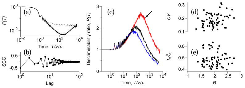
Fig. 5a shows the Fano factor for a representative afferent firing spontaneously (solid line), and for the corresponding renewal surrogate (dotted line). As predicted by the analytic theory (cf. Fig. 3a), the Fano factor of the original spike train, F_n(T), is significantly smaller than that of the renewal surrogate, F_r (T), for 10〈I〉 < T < 1000〈I〉, indicating suppressed variability in the original spike train.

FIG. 5.

(Color online) Experimental data from a paddlefish electroreceptor (PER) afferents. (a): Fano factors for the original (solid line) and renewal (dotted line) spike trains, and (b): SCCs for an afferent with mean ISI 〈I〉 = 15.8 ms, CV = 0.163, and f_e/f_a = 0.43. (c): The ratio of discriminability slopes, R(T), for three different afferents. Arrow: afferent shown in panels (a),(b). (d),(e): R at 1 s window vs. CV and vs. f_e/f_a for a population of 56 PER afferents.

We “stimulated” an afferent by inserting N spikes in random positions not already occupied by spontaneous spikes, in non-overlapping 1 s windows. This procedure increases the firing rate by N Hz, so that α = N 〈I〉. Both the original spike train and the renewal surrogate yield a linear dependence of the discriminability d′ on α described by Eq. 3 (data not shown). The slope of the discriminability at T = 1 s was 2.1-fold steeper for the original than for renewal data: thus, there was twice-better detection by the original spike train than by its renewal counterpart. The ratios of discriminability slopes R(T) are shown in Fig. 5c for three different afferents and are in excellent agreement with analytical predictions (cf. Fig. 3e).

Fig. 5d,e summarizes results for the sample of 56 PER afferents. The mean firing rate in this population was 54.43 ± 9.54 Hz, with CV = 0.19 ± 0.05. The epithelial-to-afferent frequency ratio f_e/f_a = 0.49 ± 0.07. The value of the Fano factor was 0.031 ± 0.01 at T = 150 ms, 0.010 ± 0.005 at T = 1 s. The population average of the discriminability ratio R was 1.34 ± 0.13 at T = 150 ms, 1.99 ± 0.35 at T = 1 s, indicating that discriminability was always better for a nonrenewal spike train. No significant dependence of R on CV or the frequency ratio was observed. These population results can be mapped to the parameter space of the model (Fig. 4). For the range of frequency ratios near 0.5, epithelial oscillations induce extended serial ISI anticorrelations and enhance the discriminability for realistic values of CV. This near-0.5-ratio high-Q regime corresponds to parameter values found in our PER database. The exact value of the frequency ratio is not crucial to achieve high discriminability in this regime. Hence PERs operate in a regime where reliable signal detection is possible without fine parameter tuning. Our analytical calculations agreed quantitatively with experimental data from PER revealing that coherent stochastic oscillations can enhance the discrimination performance of sensory neurons.

IV. CONCLUSION

We have studied the effect of stochastic oscillations acting as a source of external noise, on discrimination of weak signals by periodically spiking neurons. Coherent stochastic oscillations lead to serial correlations extending to several dozens of interspike intervals, with the structure determined by the ratio of the frequency of driving stochastic oscillations (f_e) and the neuron mean firing rate (f_a), and by the quality factor (Q) of driving oscillations. This mechanism for generation of serial correlations is distinct from the one described for electroreceptors of weakly electric fish [4], where negative ISI correlations appear presumably due to a negative feedback from adaptation ionic currents or modulation of firing threshold [7, 8] and do not extend beyond few interspike intervals. We demonstrate that spike count variability induced by these oscillations can be suppressed relative to a corresponding renewal model, if the frequency of driving oscillations is smaller than the mean firing rate and their coherence is large enough. Suppressed spike count variability translates to an enhanced discrimination capacity of the neuron, characterized in this study by the discriminability measure d′. Our analytical calculations yield parameter range where discriminability is enhanced by coherent stochastic oscillations.

We applied these analytical predictions to study the role of epithelial oscillations in peripheral electroreceptors of paddlefish. The population averages of the ratio of epithelial to sensory neuron frequencies and of the quality factor of epithelial oscillations are nicely mapped on the analytically derived parameter range of discriminability enhancement. This gives a strong argument in favor that epithelial oscillations serve to enhance discriminability of weak signals.

In conclusion, our analytical calculations underscore that coherent oscillations can improve discrimination capacity of spiking neurons in a feed-forward scenario. Such mechanism may be relevant to a broad range of phenomena involving unidirectionally coupled oscillators, e.g. to spiking neurons receiving feed-forward oscillatory input from a network of CNS neurons, or possibly to low-frequency sensors of electric and magnetic fields [22, 23].

References

- 1.Buzsaki G. Rhythms of the Brain. Oxford University Press; 2006. [Google Scholar]
- 2.Schaefer AT, Angelo K, Spors H, Margrie TW. PLoS Biol. 2006;4:e163. doi: 10.1371/journal.pbio.0040163. [DOI] [PMC free article] [PubMed] [Google Scholar]
- 3.Masuda N, Doiron B. PLoS Comput Biol. 2007;3:e236. doi: 10.1371/journal.pcbi.0030236. [DOI] [PMC free article] [PubMed] [Google Scholar]
- 4.Ratnam R, Nelson ME. J Neurosci. 2000;20:6672. doi: 10.1523/JNEUROSCI.20-17-06672.2000. [DOI] [PMC free article] [PubMed] [Google Scholar]
- 5.Chacron MJ, Maler L, Bastian J. Nat Neurosci. 2005;8:673. doi: 10.1038/nn1433. [DOI] [PMC free article] [PubMed] [Google Scholar]
- 6.Mar DJ, Chow CC, Gerstner W, Adams RW, Collins JJ. Proc Natl Acad Sci USA. 1999;96:10450. doi: 10.1073/pnas.96.18.10450. [DOI] [PMC free article] [PubMed] [Google Scholar]
- 7.Chacron MJ, Longtin A, Maler L. J Neurosci. 2001;21:5328. doi: 10.1523/JNEUROSCI.21-14-05328.2001. [DOI] [PMC free article] [PubMed] [Google Scholar]
- 8.Chacron MJ, Lindner B, Longtin A. Phys Rev Lett. 2004;92:080601. doi: 10.1103/PhysRevLett.92.080601. [DOI] [PubMed] [Google Scholar]
- 9.Neiman AB, Russell DF. J Neurophysiol. 2004;92:492. doi: 10.1152/jn.00742.2003. [DOI] [PubMed] [Google Scholar]
- 10.Gabbiani F, Koch C. In: Computational Neuroscience. Koch C, Segev I, editors. MIT Press; 1998. [Google Scholar]
- 11.Cox DR. The Statistical Analysis of Series of Events. Wiley; New York: 1966. [Google Scholar]
- 12.Lowen SB, Teich MC. J Acoust Soc Am. 1992;92:803. doi: 10.1121/1.403950. [DOI] [PubMed] [Google Scholar]
- 13.Middleton JW, Chacron MJ, Lindner B, Longtin A. Phys Rev E. 2003;68:021920. doi: 10.1103/PhysRevE.68.021920. [DOI] [PubMed] [Google Scholar]
- 14.Lindner B. Phys Rev E. 2004;69:022901. doi: 10.1103/PhysRevE.69.022901. [DOI] [PubMed] [Google Scholar]
- 15.Stratonovich RL. Topics in the Theory of Random Noise. Gordon and Breach; New York: 1963. [Google Scholar]
- 16.Schwalger T, Schimansky-Geier L. Phys Rev E. 2008;77:031914. doi: 10.1103/PhysRevE.77.031914. [DOI] [PubMed] [Google Scholar]
- 17.Neiman AB, Russell DF. Phys Rev E. 2005;71:061915. doi: 10.1103/PhysRevE.71.061915. [DOI] [PubMed] [Google Scholar]
- 18.Fuwape I, Neiman AB. Phys Rev E. 2008;78:051922. doi: 10.1103/PhysRevE.78.051922. [DOI] [PubMed] [Google Scholar]
- 19.Rice SO. Bell System Tech J. 1945;24:51. [Google Scholar]
- 20.Verechtchaguina T, Sokolov IM, Schimansky-Geier L. Phys Rev E. 2006;73:031108. doi: 10.1103/PhysRevE.73.031108. [DOI] [PubMed] [Google Scholar]
- 21.Risken H. The Fokker-Planck Equation. Springer; Berlin: 1996. [Google Scholar]
- 22.Acebron JA, Rappel WJ, Bulsara AR. Fluctuation and Noise Letters. 2003;3:L341. [Google Scholar]
- 23.Bulsara AR, In V, Kho A, Palacios A, Longhini P, Neff J, Anderson G, Obra C, Baglio S, Ando B. Measurement Science and Technology. 19:075203. [Google Scholar]