A surface‐based technique for mapping homotopic interhemispheric connectivity: Development, characterization, and clinical application

Abstract

The functional organization of the human brain consists of a high degree of connectivity between interhemispheric homologous regions. The degree of homotopic organization is known to vary across the cortex and homotopic connectivity is high in regions that share cross‐hemisphere structural connections or are activated by common input streams (e.g., the visual system). Damage to one or both regions, as well as damage to the connections between homotopic regions, could disrupt this functional organization. Here were introduce and test a computationally efficient technique, surface‐based homotopic interhermispheric connectivity (sHIC), that leverages surface‐based registration and processing techniques in an attempt to improve the spatial specificity and accuracy of cortical interhemispheric connectivity estimated with resting state functional connectivity. This technique is shown to be reliable both within and across subjects. sHIC is also characterized in a dataset of nearly 1000 subjects. We confirm previous results showing increased interhemispheric connectivity in primary sensory regions, and reveal a novel rostro‐caudal functionally defined network level pattern of sHIC across the brain. In addition, we demonstrate a structural–functional relationship between sHIC and atrophy of the corpus callosum in multiple sclerosis (r = 0.2979, p = 0.0461). sHIC presents as a sensitive and reliable measure of cortical homotopy that may prove useful as a biomarker in neurologic disease. Hum Brain Mapp 37:2849–2868, 2016. © 2016 Wiley Periodicals, Inc.

INTRODUCTION

The architecture of the brain consists of both intra‐ and interhemispheric connections that facilitate regionally specific processing and long‐range communication. The left and right hemispheres demonstrate a regionally varying degree of homotopy [Aboitiz et al., 1992a, 1992b; Olivares et al., 2001; Tomasch, 1954; Tomasch and Macmillan, 1957], or connectivity between homologous contralateral anatomical regions. Despite the lateralization of some cognitive processes [Toga and Thompson, 2003; Wang et al., 2014], the need to integrate sensory information and higher level cognitive processing across the hemispheres suggests that such robust and varied interconnectivity is an important feature of the cortical architecture.

Mapping intrinsic functional connectivity (iFC) by measuring coherent fluctuations in low frequency blood‐oxygen‐level dependent (BOLD) signal demonstrates regional variation in cerebral homotopy [Salvador et al., 2005]. Using this technique, homotopic regions tend to have higher connectivity relative to connectivity to nonhomotopic regions [Biswal et al, 1995]. In a targeted investigation of interhemispheric homotopy using voxel mirrored homotopic connectivity (VMHC), the primary motor, somatosensory and visual cortices demonstrated a high degree of interhemispheric coordination, while unimodal and heteromodal association cortices displayed significantly lower interhemispheric connectivity [Stark et al., 2008]. Evaluating brain connectivity across the lifespan [Zuo et al., 2010] and characterizing changes in connectivity in several disease states, including autism [Anderson et al., 2011], traumatic brain injury [Sours et al., 2015] and schizophrenia [Guo et al., 2014a, 2014b; Hoptman et al., 2012] are additional applications of homotopic connectivity.

The corpus callosum (CC) is the main white matter structure connecting the two hemispheres and tract tracing studies in animals suggest that the topography of the CC facilitates the observed largely homotopic organization of the cortex [Innocenti, 2009]. This is further supported by electrophysiological studies reporting decreased interhemispheric coupling in patients with callosal agenesis [Brown et al., 1998; Koeda et al., 1999; Nagase et al., 1994; van de Wassenberg et al., 2008] and reduced resting‐state functional connectivity following callosal transection [Johnston et al., 2008]. In multiple sclerosis (MS), an inflammatory, demyelinating disorder of the nervous system, focal lesions within the CC, and Wallerian degeneration from adjacent hemispheric white matter lesions are thought to result in atrophy of the CC [Klawiter et al., 2015]. CC atrophy occurs in tandem with atrophy in the gray matter and correlates with increasing levels of disability [Klawiter et al., 2015; Yaldizli et al., 2010] and cognitive dysfunction [Bergendal et al., 2013; Granberg et al., 2015; Llufriu et al., 2012; Lowe et al., 2008; Rao et al., 1989] in relapsing‐remitting MS (RRMS). Using VMHC to investigate homologous interhemispheric connectivity, Zhou et al. [2013] found significantly decreased homotopic connectivity in RRMS subjects compared with healthy controls and a positive correlation between VMHC values and fractional anisotropy of the CC. Using EEG, Zito et al. [2014] found evidence for a relationship between altered interhemispheric cross‐frequency coupling and CC thickness in RRMS subject performing a motor task. Together, these results suggest a link between damage to the CC in MS and changes to cerebral homotopy.

Past work using iFC to estimate homotopy has primarily used volumetric processing and registration techniques and left–right X coordinate reversal to calculate VMHC [Guo et al., 2014a, 2014b; Hoptman et al., 2012; Jakab et al., 2012; Razlighi et al., 2013; Stark et al., 2008; Zhou et al., 2010, 2013]. Here we describe the development and validation of a technique for evaluating interhemispheric homologous functional connectivity that leverages the reconstructed cortical surface, namely, surface‐based homologous interhemispheric connectivity (sHIC). Surface‐based preprocessing and registration methods [Dale et al., 1999; Fischl et al., 1999] have been shown to improve the accuracy and reliability of intersubject alignment over volumetric methods in fMRI studies [Anticevic et al., 2008; Jo et al., 2008, 2007; Tuchola et al., 2012] and increase the overlap of cytoarchitectonic boundaries between subjects [Fischl et al., 2008], albeit at the expense of limiting analyses to the cortical sheet and omitting subcortical gray matter. Surface‐based methods have been used extensively in structural and functional analyses including interhemispheric connectivity [Greve et al., 2013; Jo et al., 2012]. Jo et al. [2012] previously used landmark‐based anatomical correspondence to determine putative homologous points between the hemispheres on a non‐symmetric template brain. Our goal was to improve the assessment of regional patterns of cerebral homotopy with surface‐based registration techniques and processing methods and using a symmetric surface template for which anatomical correspondence is assured. The second aim of this work was to characterize surface‐based homotopy using a large dataset of nearly 1000 subjects. Furthermore, we hypothesized that the increased spatial specificity of sHIC would reveal a novel relationship between decreased rs‐fMRI whole‐brain homotopy in an RRMS population and atrophy of the CC in MS.

METHODS

Subject Datasets

Three separate datasets were used for this work: (1) a development and reliability dataset with scan–rescan data, (2) a large‐scale dataset of nearly 1000 healthy volunteers to define homologous connectivity patterns, and (3) a clinical application dataset of patients with MS, a group for whom alterations in homologous connectivity could be expected. Demographics for the datasets used herein are summarized in Table 1.

Table 1.

Dataset Demographic Information

Dataset	N	Age, mean ± SD (range)	Gender, M:F	Disease duration	Median EDSS (range)
Kirby21	21	31.76 (22–61)	11:10	N/A	N/A
BGSP	998	21.3 (18–35)	645:353	N/A	N/A
Clinical
HC	51	32.55 ± 9.313(20–52)	33:18	N/A	N/A
MS	33	40.21 ± 9.313(22–59)	8:25	7.774 ± 6.32 (1–20)	2.0 (0–4)

Kirby21 dataset

The dataset used for development and reliability calculation, hereafter referred to as the Kirby21 database, consisted of data from 21 healthy control (HC) subjects (mean age = 31.76, range 22–61, M:F 11:10) available in the freely downloadable Multi‐Modal MRI Reproducibility Resource (https://www.nitrc.org/projects/multimodal/) [Landman et al., 2011]. This dataset consists of subjects who were scanned twice on the same day using an identical imaging protocol. The Kirby21 dataset was used to determine the reliability of the sHIC technique by calculating voxel‐wise intraclass correlation coefficients (ICC) using the included scan–rescan resting‐state (rs‐fMRI) data.

BGSP dataset

A dataset of 998 healthy young adults subjects (mean age = 21.3, range 18–35, M:F 645:353) provided by the Brain Genomics Superstruct Project (BGSP) of Harvard University and the Massachusetts General Hospital [Buckner et al., 2011; Choi et al., 2012; Yeo et al., 2011]. The GSP dataset was used for large‐scale characterization of whole‐brain patterns of sHIC and between subject variability.

Clinical dataset

The third dataset consisted of 40 subjects who met criteria for clinically definite RRMS [Polman et al., 2005] and 59 HC subjects. The Clinical dataset was used to apply sHIC to a population where a relationship between decreased homotopic connectivity and CC integrity is expected [Zhou et al., 2013]. The HC subjects were scanned as part of the MGH/UCLA Human Connectome Project (HCP) and acquired using the Connectom (MAGNETOM Skyra CONNECTOM, Siemens Healthcare) scanner located at the Martinos Center for Biomedical Imaging, which consists of a Siemens Skyra 3 T MRI modified with an AS302 gradient system. RRMS subjects were acquired using the same scanner and pulse sequences as the HCP data. Following data quality assessment, five RRMS subjects and eight HC subjects were eliminated due to a priori exclusion criteria, including visually obvious image artifacts, inadequate signal‐to‐noise ratio (SNR), or the presence of within session movement above set thresholds (see Functional Preprocessing). Following research indicating altered intrinsic network integrity in depressed adults [Diener et al., 2012; Kerestes et al., 2014; Marchetti et al., 2012; Wang et al., 2012; Tadayonnejad and Ajilore, 2014], two additional RRMS subjects were excluded based on a priori exclusion criteria for severe depression as indicated by a total score ≥28 on the Beck Depression Inventory [Beck et al., 1988]. The remaining dataset consisted of 33 RRMS (mean age = 40.21 ± 9.52, range 22–59, M:F 8:25) and 51 HC (mean age = 32.55 ± 9.313, range 20–52, M:F 33:18) subjects. Mean disease duration for the RRMS subjects was 7.74 ± 6.32 years (range 1–20) with a median Expanded Disability Status Scale of 2.0 (range 0–4). All RRMS subjects were free of relapses in the three months prior to study entry. Subjects with a history of psychiatric or neurological conditions other than MS were excluded from the study. All subjects provided written informed consent in accordance with the guidelines set by the institutional review board of Partners Healthcare.

MRI Acquisition

Each subjects' data from the Kirby21 dataset consisted of two separate sessions acquired on the same Phillips 3 T Achieva scanner (Philips Healthcare, Best, The Netherlands) equipped with an 8‐channel phase array SENSitivity Encoding (SENSE) head coil. High‐resolution 3D T1‐weighted (T1w) magnetization‐prepared rapid acquisition gradient echo (MPRAGE) anatomical images (repetition time (TR)/echo time (TE)/inversion time (TI) = 6.7/3.1/842 ms, field of view (FOV) = 240 × 204 × 256 mm, flip angle (FA) = 8°, SENSE = 2, 1 × 1 × 1.2 mm voxel resolution, acquisition time (TA) = 5:56) were used for registration and cortical surface reconstruction. rs‐fMRI images were acquired using a 2D gradient‐echo (GE) echo‐planar imaging (EPI) sequence sensitive to BOLD contrast (TR/TE = 2000/30 ms, FA = 75°, SENSE = 2, 37 transverse slices in ascending order, 1 mm slice gap, 3 mm isotropic voxel resolution, 210 time points, TA = 7:00). This dataset, along with demographic data, is freely downloadable from Neuroimaging Informatics Tools and Resources Clearinghouse (http://www.nitrc.org). See Landman et al. [2011] for additional details and further description of acquisition parameters.

The BGSP dataset was acquired on 3 T Siemens Tim Trio scanners (Siemens, Erlangen, Germany) located at Harvard University and Massachusetts General Hospital and equipped with a 12‐channel phased array head coil. A 3D multiecho (ME) MPRAGE [van der Kouwe et al., 2008] sequence (TR/TEs = 2200/1.45–7.01 ms, FOV = 230, FA = 7°, 1.2 mm isotropic resolution) was used for registration and cortical reconstruction. One or two 2D GE EPI sequences sensitive to BOLD contrast were acquired per subject (TR/TE = 3000/30 ms, FOV = 216, FA = 85°, 3 mm isotropic voxel resolution, 47 axial slices with interleaved acquisition, no slice gap, 124 time points, TA = 6:12) as scan time allowed. The rs‐fMRI run with the highest SNR was chosen for inclusion in the study.

The Clinical dataset was acquired on the 3 T Connectom scanner at MGH using a 64‐channel phased array head coil [Keil et al., 2013]. Pulse sequence protocols for RRMS subjects were matched to those used for the MGH/UCLA HCP dataset. A high‐resolution 3D T1w MEMPRAGE sequence (TR/TE/TI = 2530/[1.15, 3.03, 4.89, 6.75]/1100 ms, FOV = 256, FA = 7°, 1 mm isotropic voxel resolution, GRAPPA acceleration (R) = 2) was acquired for use in registration, cortical surface reconstruction, and quantification of CC area in RRMS subjects. High‐resolution 3D T2‐weighted (T2w) images (TR/TE = 3200/561 ms, FOV = 224, variable FA, 0.7 mm isotropic voxel resolution, R = 2, BW = 744 Hz, TA = 5:57 min) were acquired to aid in estimation of the pial‐gray matter boundary during cortical reconstruction. rs‐fMRI images were acquired using a 2D single‐shot GE EPI sequence sensitive to BOLD contrast (TR/TE = 3000/30 ms, FOV = 214, FA = 85°, 3 mm isotropic resolution, 47 interleaved slices, 120 measurements, BW = 2240 Hx, TA = 6:06 min). Foam padding was used to restrict head motion and earplugs were supplied to attenuate scanner noise. Subjects were instructed to lie still within the scanner for the duration of the scan, keep their eyes open, and to let their minds wander but not to fall asleep.

MRI Preprocessing

Figure 1 provides the schematic overview of the anatomical and functional preprocessing and integration.

Figure 1.

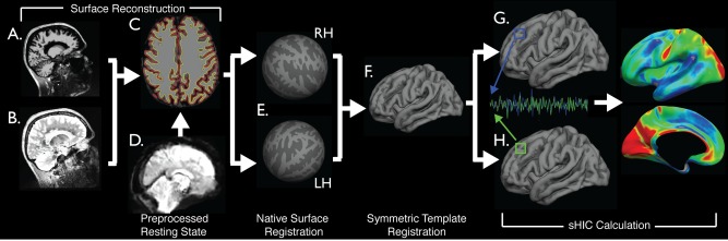
Schematic representation of processing pipeline. Preprocessed T1w (A) and T2w (B) images were processed with FreeSurfer (C) to obtain cortical surface reconstructions (E) and then registered to a symmetric template (F). Preprocessed functional data (D) was resampled to the template via each individual subjects' native anatomy (E–G). Homotopic connectivity was calculated using data sampled to a single hemisphere (G–I). [Color figure can be viewed in the online issue, which is available at http://wileyonlinelibrary.com.]

Gradient nonlinearity correction

Prior to processing via the standard Freesurfer cortical reconstruction pipeline, T1w and T2w images were corrected for gradient nonlinearity geometric distortions as previously described [Jovicich et al., 2006; Cannon, 2014] and coregistered using boundary‐based registration (BBR) [Greve & Fischl, 2009].

Anatomical surface reconstruction

The Kirby21 and Clinical datasets, both of which included T1w and T2w images, were processed using Freesurfer (version 5.3, http://surfer.nmr.mgh.harvard.edu/) [Dale et al., 1999; Fischl et al., 1999] and in‐house developed scripts. Following initial processing through the Freesurfer pipeline (Fig. 1A–C), the resulting cortical surface reconstructions were assessed by an experienced user, manually edited, and recalculated prior to further analysis. MS subjects from the Clinical dataset received particular attention due to automated methods of establishing the white matter/gray matter (WM/GM) boundary misinterpreting lesioned hypointense WM erroneously as GM. Lesioned tissue in the WM was hand edited to reclassify it as WM in these cases. The BGSP dataset was previously reconstructed using Freesurfer v.4.5 [Yeo et al., 2011].

Surface‐based cross‐hemisphere registration

Surface‐based registration [Fischl et al., 1999] aligns the cortical folding patterns of an individual to match the gyral/sulcal pattern of an ipsilateral template. Surface‐based registration has been shown to be superior to volume‐based registration methods [Fischl et al., 2008] in the cortex. Greve et al. [2013] further developed these techniques to create an unbiased symmetric template and register each hemisphere of the individual to this symmetric space to perform interhemispheric analyses. We used these interhemispheric routines (http://surfer.nmr.mgh.harvard.edu/fswiki/Xhemi) to register each hemisphere to the “fsaverage_sym” symmetric surface template distributed with FreeSurfer (Fig. 1E,F) to provide the interhemispheric correspondence need to perform our iFC analyses. Each subject's left hemisphere was first registered to the left hemisphere of the template, followed by registration of the subject's right hemisphere to the template left hemisphere. The resulting surfaces for each subject then consisted of two left‐hemisphere‐registered surfaces in a standard space. Alternatively, both hemispheres can be mapped to the right template hemisphere. Greve et al. [2013] verified that these two methods generated the same results for thickness analysis. We furthered this validation by testing for differences in iFC related to using either the left or right template hemisphere (Supporting Information, Fig. 1).

Volume‐Based Symmetric Template Creation

Scan 1 data from the Kirby21 dataset was used to create a study specific volume in the fashion of Zuo et al. [2010]. Briefly, the T1w image from each subject was nonlinearly registered to the MNI152 1 mm atlas using FLIRT/FNIRT and then averaged together. A left–right reversed version was created by reversing the x‐coordinate of this average image using fslswapdim and then averaging with the original image. The MNI registered, individual subject T1w images were then reregistered to the symmetric template, followed by refining the original registration by concatenating the two nonlinear registrations together. This registration was then used in the processing of the Kirby21 resting‐state data.

CC Morphometry

High‐resolution MEMPRAGE images from the Clinical dataset were additionally preprocessed through a volumetric morphometry pipeline before analyzing callosal morphology. T1w images were corrected for gradient nonlinearity, intensity normalized to account for bias field inhomogeneity [Sled et al., 1998; Zheng et al., 2009], and registered to MNI152 space using a 6 degree of freedom rigid body transformation performed with FSL's Linear Image Registration Tool (FLIRT) [Jenkinson et al., 2002]. This registration step was performed to account for subject specific off‐axis head alignment, facilitate callosal area calculations on the same mid‐sagittal slice across subjects, and avoid any scaling of the CC. Scans were then segmented by tissue type using FMRIB's Automated Segmentation Tool (FAST v.4) [Zhang et al., 2001], including partial volume estimation (PVE). The midsagittal slice of the WM PVE map was extracted from the whole volume, thresholded to remove voxels that contained less than 30% WM and binarized. The resulting WM maps were hand edited to remove any remaining non‐callosal WM, which typically consisted of brainstem, fornix, the anterior and/or posterior commissures and large medial vessels, and to replace areas of hypointense WM lesion erroneously removed by the algorithm. The area of the mid‐sagittal CC (CCA) was then calculated by summing the remaining voxels and normalizing this area by dividing by the estimated total intracranial volume (eTIV)^(2/3), as determined by Freesurfer.

Resting‐state preprocessing

Functional image preprocessing for the Kirby21 and Clinical datasets was conducted in the volume in native space using FSL and in‐house developed tools before resampling the data to the symmetric template and performing smoothing along the geodesic surface. Preprocessing steps for the Kirby21 dataset included removal of the first 4 timepoints to account for T1 equilibration, compensation for slice‐time dependent shifts due to ascending acquisition, and affine registration of each volume of the timeseries to the first volume (following time point removal) to account for subject head motion. Preprocessing of the Clinical dataset proceeded in a different order due to the necessity to correct for the additional gradient nonlinearity distortion present in the Connectom scanner. Preprocessing steps for the Clinical dataset included removal of the first 4 timepoints, slice‐timing correction to account for interleaved acquisition, combined gradient nonlinearity correction and motion correction and grand mean intensity normalization. The Kirby21 and Clinical datasets were further processed by applying a fourth‐order Butterworth temporal bandpass filter to remove linear trends and isolate BOLD oscillation frequencies between 0.001 and 0.08 Hz. Signal contamination by spurious physiological artifacts and non‐neuronal contributions were removed by multiple regression. Factors regressed from the data included the six rigid body head motion parameters calculated during motion correction, their first temporal derivatives and the square of each of these 12 regressors. Additional factors included the mean signal and the first 5 components from a PCA analysis of signal extracted from FreeSurfer derived masks of the WM and ventricles [Behzadi et al., 2007]. To account for the effect of large, single‐head movements in the scanner, framewise displacement [Power et al., 2012] was used to calculate the relative movement at each timepoint, in reference to the previous timepoint. The global signal was not regressed from the iFC time series.

For all datasets, the subject was excluded if any of the following criteria were met: (1) functional SNR level < 150, (2) maximal absolute displacement > 1.5 mm, (3) average framewise displacement (timepoint to timepoint) > 0.5 mm, (4) greater than 5% of timepoints identified as movement outliers (framewise displacement > 0.5 mm), or (5) presence of significant image artifacts (e.g., significant EPI ghosting).

Functional‐surface registration

Each subject's functional data from the Kirby21 and Clinical datasets (Fig. 1D) were registered to their anatomical data in native space using BBR (Fig. 1E) [Greve and Fischl, 2009]. rs‐fMRI data were then resampled onto the symmetric template using this registration and the previously calculated spherical surface registration between the subjects' reconstructed cortical surface and the symmetric surface template (Fig. 1D–F). This was accomplished in a single interpolation step that sampled data from the middle of the cortical ribbon to the tessellated mesh surface. Data were smoothed on the surface using a 4 mm FWHM Gaussian smoothing kernel. Functional data from the BGSP dataset were previously registered to the Freesurfer fsaverage6 surface template and smoothed with a 6 mm smoothing kernel [Yeo et al., 2011]. The spherical registration between the fsaverage 6 template and the symmetric template was then calculated and the functional data were resampled into the symmetric fsaverage_sym template space.

Surface‐Based Homotopic Interhemispheric Connectivity

Following preprocessing and coregistration of the functional data with the symmetric surface template, sHIC was calculated using in‐house developed code written in MATLAB (version 8.2, Natick, Massachusetts: The MathWorks Inc., 2013). Homologous vertices were defined as pairs of vertices that shared the same Freesurfer‐assigned index and spatial location on the symmetric template (Fig. 1G,H). The pairwise Pearson's correlation between the extracted timecourse for each member of each pair of vertices was calculated, thus generating a metric of homologous connectivity per surface vertex (Fig. 1I). Correlation values were normalized using Fisher's r‐to‐Z transformation prior to group comparison. Code for conducting the sHIC analysis is available from the authors upon request.

Alternative Homotopic Calculation

To test whether single vertex homotopy is able to adequately capture the contralateral homotopic region, an alternative method, termed nearest neighbor sHIC (nn‐sHIC), was developed. Prior to cross‐hemisphere correlation, each vertex and its immediate neighbors were combined into a single region of interest (ROI) to provide a larger seed region. The same procedure was used for the contralateral homologous vertex to provide a larger target region. Signal from each multi‐vertex ROI was extracted and used to calculate sHIC. The Fisher normalized correlation value between the larger seed and target regions was assigned to the original central seed vertex.

Volume‐Specific Resting‐State Processing

To facilitate comparison between sHIC and VMHC, Scan 1 Kirby21 rs‐fMRI data were additionally preprocessed using a pipeline that incorporated volumetric smoothing. Following time point removal, slice‐timing correction, and motion correction as previously detailed, data were smoothed with a 6 mm FWHM 3D Gaussian kernel and the registration between each subject's rs‐fMRI data and their native T1w image was calculated using FLIRT + BBR. This linear registration was then concatenated with the nonlinear registration between the T1w image and the symmetric template (see Volume‐based Symmetric Template Creation). Remaining preprocessing steps, including bandpass filtering and denoising, were completed as previously detailed. The fully preprocessed rs‐fMRI data were nonlinearly registered to the symmetric volume template using this transform. These data were used for the calculation of VMHC using REST version 1.8 MATLAB software [Song et al., 2011]. VMHC results were averaged and mapped from the symmetric volume template to the symmetric surface template using surface‐based registration.

Alternately, rather than transforming the preprocessed data to the symmetric volume template, the volume‐smoothed, preprocessed resting‐state data were resampled to the symmetric surface template using the surface registration calculated during processing for sHIC (see Functional Surface Registration). These data were used for the calculation of volume‐smoothed sHIC using the same surface‐based methods developed for surface‐smoothed sHIC. No additional surface smoothing was applied during resampling. Final results were averaged across subjects for comparison with sHIC and VMHC. When the above analyses were complete, each Kirby21 subject possessed results for three separate analysis streams: sHIC, VMHC, and sHIC calculated with volume‐smoothed data.

Cortical Parcellation Extraction

Several structural and functional parcellation schemes were used to investigate patterns of sHIC across the cortex. Probabilistic Brodmann areas were used to analyze motor and sensory cortex [Fischl et al., 2008], however, owing to the large size of Brodmann areas 17–19, several more fine‐grained visuotopic regions from the PALS‐B12 surface [Van Essen, 2005] were used to investigate visual cortex. Auditory cortex was investigated using a three region parcellation of Heschel's gyrus (http://web.mit.edu/svnh/www/Resolvability/ROIs.html) [Norman‐Haignere et al., 2013]. Finally, a functionally parcellation derived from rs‐fMRI data was used to analyzed cortical network‐level sHIC [Yeo et al., 2011]. All parcellations were mapped to the symmetric left hemisphere template from either fsaverage surface space or MNI152 volume space using spherical registration.

In addition to the average homotopic connectivity for the whole brain, several regions of interest were selected to evaluate the sHIC, VMHC, and volume‐smoothed sHIC analyses for differences. V1 [Van Essen, 2005] was selected for the expected high degree of homotopy across the hemispheres. Brodmann area 44 (BA44) [Fischl et al., 2008] and the dorsal anterior cingulate cortex (dACC) were selected for their expected low homotopy. BA44, or Broca's area is commonly described as a left lateralized language region, while dACC has been shown to be strongly right lateralized [Wang et al., 2015]. Finally, a medial surface ROI was constructed by manually outlining the medial aspect of the symmetric surface template pial surface, followed by subtraction of medial wall vertices (i.e., the “cut” FreeSurfer must perform through the midline to separate the two hemispheres). The border of the medial surface ROI was placed at the distinct change in curvature observed when wrapping from medial to more lateral cortex, as seen in the sagittal view of the symmetric surface. The parahippocampal gyrus was omitted from the medial surface ROI. The medial surface ROI was created to specifically to examine differences in medial surface homotopy.

Statistics

Statistical analyses were conducted using MATLAB. ICC values were calculated for each vertex v according to the following equation: ICC_v =  $\frac{{\mathrm{M}\mathrm{S}}_{\mathrm{p}}‐ {\mathrm{M}\mathrm{S}}_{\mathrm{E}\mathrm{i}}}{{\mathrm{M}\mathrm{S}}_{\mathrm{p}}+\left(k‐1\right){\mathrm{M}\mathrm{S}}_{\mathrm{e}}}$, where MS_p is the group mean square, MSE is the individuals mean square error, and k is the number of observations (herein 2 acquisitions). Significant clusters of cortical sHIC were cluster corrected for multiple comparisons [Hagler et al., 2006]. Extracted sHIC values for the somatomotor and visual cortex were compared separately using an ANOVA with Tukey's posthoc test for significance. Values for total CCA and sHIC averaged across the entire hemisphere were correlated using a Pearson correlation. Group comparisons for differences in CCA and sHIC between MS and HC groups were conducted with a Student's t‐test and Holm–Bonferroni corrected.

RESULTS

Technical Development, Test–Retest Reliability, and Between‐Subject Variability

Template target hemisphere

The effect of registering data either to the left or to the right hemisphere of the symmetric atlas (Fig. 1D–F) was tested using the Kirby21 dataset. The resulting pattern of group average homotopic connectivity was nearly identical between the two registration targets (Supporting Information, Fig. 1). The left hemisphere was chosen as the target hemisphere for all subsequent analyses.

Smoothing

The effect of smoothing was investigated by processing the Scan 1 data of the Kirby21 dataset using a 2, 4, 6, or 8 mm kernel (Supporting Information, Fig. 2). A 2 mm kernel produced noisy final results, most likely due to the lower SNR of minimally smoothed data. While the 6 and 8 mm kernels resulted in severely blurred results, the 4 mm kernel retained a degree of spatial specificity that is potentially useful in detecting small changes in homotopic connectivity in clinical populations. The overall pattern of sHIC was preserved between the 4, 6, and 8 mm smoothing kernels. To balance spatial specificity with SNR, a 4 mm kernel was used for all subsequent analyses.

Nearest‐neighbor sHIC

The triangular mesh to which the functional data is mapped results in a higher density sampling of point‐to‐point connectivity between the hemispheres than in volumetric analyses. When nn‐sHIC is computed as detailed herein, it appears similar to standard sHIC performed on data preprocessed with an 8 mm smoothing kernel, but maintained the same pattern of high and low homotopic connectivity (Supporting Information, Fig. 3). nn‐sHIC was deemed to be inferior to standard sHIC due to this additional blurring and loss of spatial specificity.

Scan–rescan reliability

The Kirby21 dataset was used to test the scan–rescan reliability of the sHIC method. Average sHIC across the Kirby21 subjects are displayed separately for Scan 1 and Scan 2 in Figure 2A,B, respectively. The overall pattern of sHIC in the group maps was highly similar between the scanning sessions. The ICC value for each vertex was calculated using all pairs of scans for all subjects (Supporting Information, Fig. 4). The majority of the cortex had a moderate to high (>0.5) ICC value, revealing the method to be highly reliable between scanning sessions.

Figure 2.

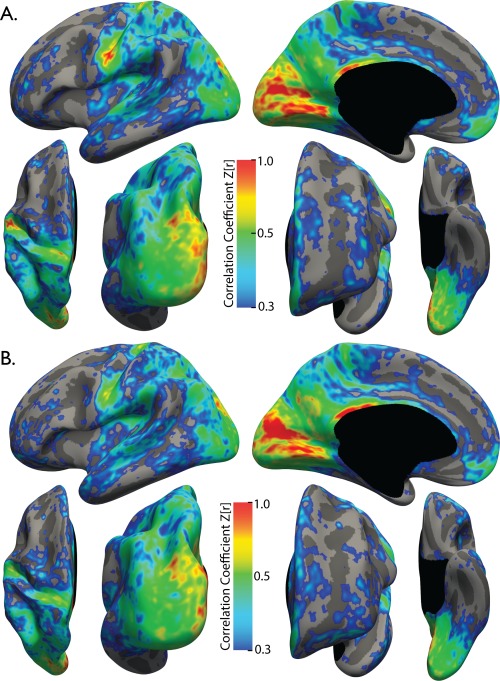
Average sHIC for the Kirby21 dataset. The pattern of homotopic connectivity is highly consistent between Scan 1 (A) and Scan 2 (B). N = 21 for each group.

Variability

The vertex‐wise coefficient of variation (CV) was calculated on 499 randomly selected subjects from the BGSP dataset (Supporting Information, Fig. 5A). The most variable regions include the orbitofrontal, posterior middle frontal gyrus and inferior frontal gyrus, subcallosal cortex, anterior inferior insula, inferior supramarginal gyrus, transverse temporal gyrus, inferior temporal gyrus, anterior collateral sulcus, middle cingulate gyrus, and parahippocampal gyrus. Other than these regions of elevated variability, the vast majority of the cortex demonstrated low CV.

In addition, average sHIC for the BGSP subjects randomly selected for the above CV calculation (Supporting Information, Fig. 5A) was compared to average sHIC for the remaining 499 subjects (Supporting Information, Fig. 5B). Minute areas of difference between the two groups were observed, producing nearly identical group average images. Plotting all vertices from all subjects of group A against all vertices from all subjects from group B reveals a nearly perfect correlation between the two (rho = 0.9987, p < 0.0001) (Supporting Information, Fig. 5C). Owing to the similarity between groups, all BGSP subjects were combined into a single group for the remaining analyses using the BGSP dataset.

Comparisons between VMHC, sHIC, and Volume‐Smoothed sHIC

Figure 3A displays the average results for calculating VMHC, sHIC, and a version of sHIC calculated using volumetric smoothing on the Scan 1 data from the Kirby21 dataset. The three techniques were found to produce qualitatively different results. Between VMHC and sHIC techniques, there is general agreement in several regions of high interhemispheric connectivity in primary motor, sensory and visual cortices, posterior cingulate cortex, and precuneus; and low homotopy in several prefrontal regions including anterior insula and temporoparietal junction. There are also substantial differences between VMHC and sHIC within the fundus of the central sulcus and along much of the gyral crowns of the medial surface. Volume‐processed sHIC revealed substantially higher interhemispheric connectivity values across the entirety of the brain, and especially so on the medial surface. Comparing sHIC over the entire brain revealed that volume‐processed sHIC produced significantly higher interhemispheric connectivity values than both VMHC and sHIC (F(2,60) = 55.71, p < 0.0001; Tukey's HSD posthoc, both p < 0.0001]; however, while average whole‐brain VMHC was higher than whole‐brain sHIC, this difference was not significant (p = 0.1308).

Figure 3.

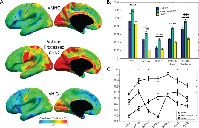
Comparison between interhemispheric techniques. (A) Average VMHC, volume‐processed sHIC, and sHIC for the Kirby 21 Scan 1 dataset. Several regions that differ between VMHC and sHIC are visible, most notably on the medial surface. (B) Whole‐brain volume processed sHIC values were significantly higher than both sHIC and VMHC. Extractions from several regions of interest reveal that, when compared to sHIC, VMHC estimates higher interhemispheric connectivity on the medial surface (i.e., dACC and medial surface ROIs), but not the lateral surface (i.e., v1, BA44) or V1. (C) The profile of interhemispheric connectivity in somatomotor cortex (BA6–BA2) calculated with VMHC demonstrated a significant dip in BA3a/p when compared to surface‐based methods, potentially due to inaccuracies introduced during volumetric template creation and registration. *p < 0.001, **p < 0.0005, corrected.

Comparisons performed between the three techniques using ANOVAs and specific ROIs found significant differences in V1 [F(2,60) = 14.06, p < 0.0001], dorsal anterior cingulate cortex [F(2,60) = 17.54, p < 0.0001], BA44 [F(2,60) = 15.51, p < 0.0001], and the medial surface [F(2,60) = 33.76, p < 0.0001] (Fig. 3B). VMHC values were correlated with cortical curvature values calculated by FreeSurfer (r = 0.2763, p < 0.0001), while sHIC and volume‐processed sHIC were not significantly correlated (r = 0.0609 and 0.053, respectively). The profile of interhemispheric connectivity across motor and sensory regions (i.e., moving caudally from BA6 to BA2) was different between each technique (Fig. 3C). While volume‐processed sHIC demonstrated decreasing patterns of interhemispheric connectivity as a function of distance from BA3a and BA3p, VMHC demonstrated a pronounced decrease in interhemispheric connectivity within BA4p and BA3a.

Anatomically Defined Patterns of Surface‐Based Homotopy

The entirety of the BGSP dataset was used to explore the large‐scale and regional patterns of homotopic connectivity between the left and right hemispheres (Fig. 4). Overall, sHIC was found to be highest in the primary and secondary motor, sensory and visual cortices. Retinotopic regions of the parietal lobe extending from V3 up the intraparietal sulcus (IPS) to IPS4 were also high in homotopic connectivity, as were regions of the superior parietal lobule, supramarginal gyrus, and posterior angular gyrus. Medially, the precuneus, parieto‐occipital sulcus, anterior and posterior cingulate gyrus, and ventromedial prefrontal cortex were also high. sHIC values were averaged and extracted using several structural and functional parcellation methods to better characterize the more focal, regional patterns of homotopic functional connectivity and are summarized in Table 2.

Figure 4.

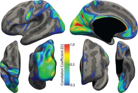
Average sHIC for the BGSP dataset. The pattern of homotopic connectivity is displayed for all 998 subjects of the BGSP dataset. The threshold is set at 0.3 to illustrate regions that are relatively high in homotopic connectivity.

Table 2.

Surface‐based Homotopic Interhemispheric Connectivity Parcel Extractions

Network/region	Abbreviation	Mean Z ± SD	p‐value
Motor cortex		0.1981 ± 0.0911	0.0073
Anterior BA3	aBA3	0.4100 ± 0.1350	<0.0001
Posterior BA4	pBA4	0.3230 ± 0.1175	<0.0001
Anterior BA4	aBA4	0.2645 ± 0.1012	<0.0001
BA6		0.1950 ± 0.0553	<0.0001
Sensory cortex		0.3203 ± 0.0497	0.0079
Posterior BA4	pBA3	0.3762 ± 0.1158	<0.0001
BA3		0.3039 ± 0.1240	<0.0001
BA4		0.2810 ± 0.0910	<0.0001
Visual cortex		0.4647 ± 0.0952	<0.0001
V1		0.5850 ± 0.1715	<0.0001
V2 dorsal	V2d	0.5229 ± 0.1958	<0.0001
V2 ventral	V2v	0.4880 ± 0.1611	<0.0001
V3		0.5464 ± 0.1745	<0.0001
V3A		0.5319 ± 0.1619	<0.0001
V4		0.3700 ± 0.1387	<0.0001
V7		0.4264 ± 0.1603	<0.0001
V8		0.2897 ± 0.1193	<0.0001
VP		0.4219 ± 0.1585	<0.0001
Nonsensory
BA44		0.1894 ± 0.0714	<0.0001
BA45		0.2172 ± 0.0722	<0.0001
Dorsal attention network		0.2911 ± 0.0661	<0.0001
Inferior precentral sulcus	iPCS	0.2100 ± 0.0972	<0.0001
Intraparietal sulcus	IPS
Anterior	aIPS	0.2874 ± 0.0870	<0.0001
Lateral occipital	LOC	0.2224 ± 0.0781	<0.0001
Retinotopic	rIPS	0.3736 ± 0.0949	<0.0001
Superior precentral sulcus	sPCS	0.2151 ± 0.0716	<0.0001
Ventral attention network		0.2177 ± 0.0536	<0.0001
Insula	INS	0.1985 ± 0.0595	<0.0001
Middle cingulate cortex	MCC	0.2180 ± 0.0723	<0.0001
Middle frontal gyrus/superior frontal sulcus	MFG/SFS	0.2143 ± 0.1603	<0.0001
Posterior cingulate cortex	PCC	0.2513 ± 0.0810	<0.0001
Posterior middle frontal gyrus	pMFG	0.2415 ± 0.1057	<0.0001
Posterior middle temporal gyrus	pMTG	0.1735 ± 0.1061	<0.0001
Temporparietal junction	TPJ	0.2411 ± 0.0954	<0.0001
Frontoparietal control network		0.2706 ± 0.0556	<0.0001
Anterior cingulate cortex	ACC	0.1777 ± 0.0770	<0.0001
Anterior insula	aINS	0.2171 ± 0.0967	<0.0001
Cingulate sulcus	CingS	0.4568 ± 0.2007	<0.0001
Inferior temporal cortex	ITC	0.1643 ± 0.0947	<0.0001
Lateral frontal cortex	LFC	0.2163 ± 0.0662	<0.0001
Posterior parietal cortex	PPC	0.3181 ± 0.0916	<0.0001
Superior frontal gyrus	SFG	0.1851 ± 0.0888	<0.0001
Superior parietal lobule	SPL	0.5009 ± 0.1457	<0.0001
Ventral prefrontal cortex	vPFC	0.2151 ± 0.0716	<0.0001
Default mode network		0.2632 ± 0.0499	<0.0001
Angular gyrus	ANG	0.2804 ± 0.0855	<0.0001
Dorsomedial prefrontal cortex	dmPFC	0.2596 ± 0.0621	<0.0001
Lateral temporal cortex	LTC	0.1758 ± 0.0609	<0.0001
Precuneus	PREC	0.4117 ± 0.0896	<0.0001
Ventrolateral prefrontal cortex	vlPFC	0.2169 ± 0.0666	<0.0001

p values correspond to the significance of Student's t‐tests against the null hypothesis that the mean value is 0.

Motor and sensory cortex

Extracting sHIC values averaged over probabilistic Brodmann areas mapped to the symmetric template confirmed the observation of high homotopy within primary motor and sensory cortices. In motor regions, sHIC descended significantly in magnitude from anterior BA3 to posterior BA4 to anterior BA4 and finally to BA6 (Table 2 and Fig. 5A,B), revealing a pattern of diminishing homotopy as distance from the primary motor cortex increased (i.e., moving anteriorly from the fundus of the central sulcus towards the frontal lobe). Sensory cortices displayed a similar pattern of sHIC, descending from posterior BA3 to BA1 and finally BA2. Nonsensory cortex within BA44 and BA45 commonly described as Broca's area and associated with lateralized language processes, possessed low homotopic connectivity.

Figure 5.

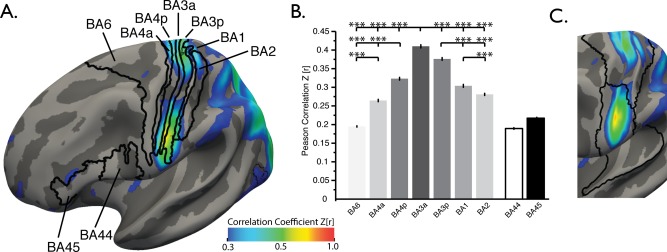
Primary motor and somatosensory sHIC. (A) Average sHIC from the BGSP dataset displayed with probabilistic Brodmann areas. (B) Extracting average sHIC from Brodmann areas revealed a pattern of decreasing homotopy from BA3a to BA6, anteriorly [F(3,3988) = 731.04, p < 0.0001 (corrected), Tukey HSD posthoc], and from BA3a to BA2, posteriorly [F(2,2991) = 199.27, p < 0.0001]. (C) The division between superior and inferior clusters of high sHIC in somatomotor regions corresponds to the border between two parcellated areas as defined in Yeo et al. [2011] [see also Power et al., 2011]. ***p < 0.0001, Tukey's HSD post hoc test.

Two separate clusters of high sHIC in superior and inferior motor regions were visible within the anterior and inferior portions of the central sulcus. The division between the two clusters corresponds with the location of a border dividing the superior and inferior somatomotor cortex parcels as estimated in two separate functional connectivity‐based parcellations of the cortex [Power et al., 2011; Yeo et al., 2011] (Fig. 5C), indicating that this division may have network‐level implications.

Visual cortex

Similar to motor and sensory cortices, sHIC diminished in magnitude as a function of distance from primary visual cortex (Table 2 and Fig. 6A–C). With the exception of the dorsal division of V2 (V2d), all visuotopic areas demonstrated a significantly decreasing pattern of sHIC (Fig. 6C) moving dorsally from V1 to dorsal V2 to V3 to V3A and finally V7. Moving ventrally, sHIC decreased from V1 to ventral V2 to VP to V4 and finally V8.

Figure 6.

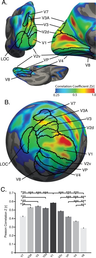
Primary visual cortex sHIC. Average sHIC from the BGSP dataset displayed with probabilistic visuotopic areas on a slightly inflated (A) and spherical (B) cortical surface for visualization. (C) Extracting average sHIC from visuotopic regions reveals a pattern of decreasing homotopy from V1 to V7, dorsally, and from V1 to V8, ventrally [F(8,8973) = 346.86, p < 0.0001]. ***p < 0.0001, corrected, Tukey's HSD posthoc test.

Auditory cortex

Primary auditory cortex demonstrated low sHIC values compared to primary motor, sensory, and visual cortices (Table 2, Supporting Information, Fig. 6). Extractions from the three divisions of Heschel's gyrus revealed low sHIC values. The planum polare and planum temporale, although included in the parcellation, were not included in this analysis.

Functionally Defined Patterns of Surface‐Based Homotopy

Mean network‐wide sHIC was also calculated for several networks characterized by recent efforts to parcellate the brain using rs‐fMRI [Yeo et al., 2011], herein specifically using the 7‐network parcellation. Mean sHIC was extracted from regions corresponding to the default mode (DMN), dorsal attention (DAN), ventral attention (VAN), and frontoparietal control (FPC) networks (Fig. 7A). The somatomotor and visual network parcellations, as defined in the 7‐network parcellation, where not analyzed, deferring to the structurally based parcellations described above. The limbic network regions were omitted due to the observed high CV and suspected high susceptibility artifact therein. When averaged over each network, sHIC values ranged from 0.2177 to 0.2911 (Table 2); and were significantly lower than sHIC values from the motor, sensory, and visual structural parcellations (all p's < 0.0001, Tukey's‐HSD post hoc). It was generally observed that the posterior nodes of each network had higher sHIC than the anterior regions (Fig. 4). Therefore, in addition to whole network values, each network was divided into its individual components and average sHIC values were extracted from each node. Additional network‐specific results are supplied in Supporting Information.

Figure 7.

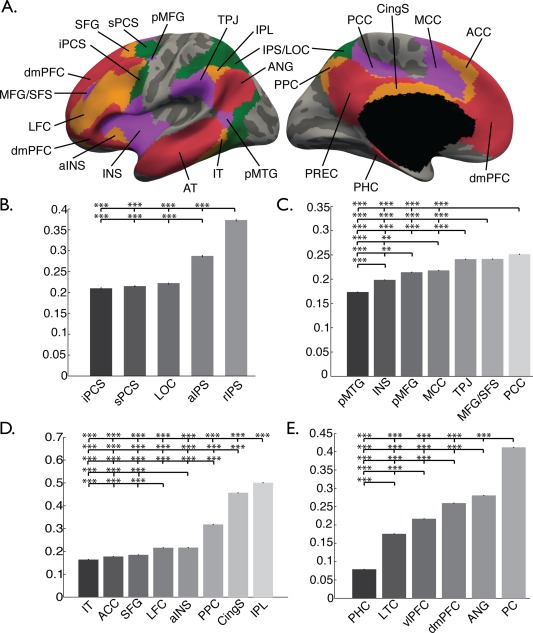
Functional surface parcellation. Regions chosen from the DAN, VAN, FPC, and DMN parcellations from Yeo et al. [2011] are displayed on lateral and medial surfaces (A). Abbreviations correspond to those regions outlined in Table 2. Average sHIC from each parcel within the (B) DAN, (C) VAN, (D) FPC, and (E) DMN is displayed in the bar graphs. **p < 0.001, ***p < 0.0001, corrected.

Callosal Atrophy and Homotopic Connectivity

CCA measurements were conducted on the midsagittal slice of the T1w data for all subjects from the Clinical Dataset (Fig. 8A). CCA was decreased in the MS group compared to the HCs (0.0498 vs 0.0562, p < 0.001) (Fig. 8B), as has been observed previously [Bergsland et al., 2012; Granberg et al., 2015; Klawiter et al., 2015]. Average sHIC is plotted for the HC and MS groups in Figure 9A. The HC group demonstrated significantly higher mean global sHIC (0.4118 ± 0.0515) compared to the MS group (0.3941 ± 0.0540) (z = 1.7358, p = 0.0413) (Fig. 9B). As hypothesized, analysis of the MS subjects revealed a significant relationship between CCA and whole cortex sHIC (r = 0.2979, p = 0.0461) while HC subjects showed no relationship (r = 0.1972, p = 0.1694) (Fig. 10).

Figure 8.

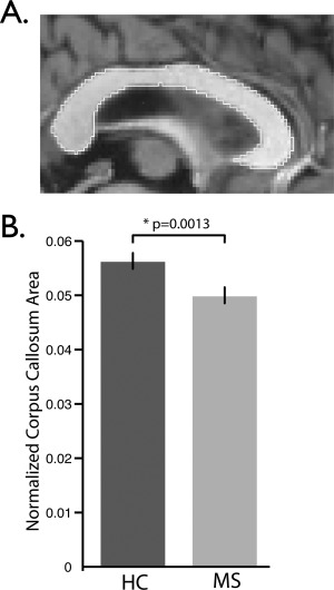
Corpus callosum area measurements. Midsagittal corpus callosum area (CCA) for representative HC subject. The border of the corpus callosum is shown in white. All voxels within the border contribute to the area measurements. (C) Average normalized CCA comparison between HC (N = 51) and MS (N = 33) groups. Normalized CCA was decreased in the MS group (p = 0.0013).

Figure 9.

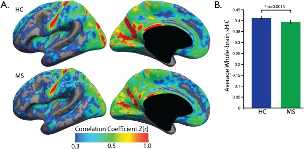
Average whole‐brain sHIC comparison. (A) Average sHIC is displayed for the HC and MS groups. (B) Mean sHIC is averaged over the entire cortex with the MS group demonstrating significantly lower average cortical sHIC compared to healthy controls (p = 0.0413).

Figure 10.

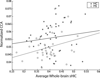
Relationship between callosal area and homotopic connectivity. Average whole‐brain sHIC and normalized CCA were not significantly correlated in the HC group (r = 0.1972, p = 0.1694, N = 51). A significant positive correlation did exist between sHIC and CCA in the MS group (r = 0.2979, p = 0.0461, N = 33).

DISCUSSION

We developed and tested a computationally efficient method for evaluating homotopic connectivity across the neocortex using surface‐based methods for data preprocessing and analysis. We characterized the patterns of cerebral homotopy as revealed by surfaced‐based methods, finding a more nuanced and regionally specific pattern than previously observed. Finally, we applied our validated method by evaluating the relationship between whole‐brain homotopic connectivity and CC atrophy in an RRMS dataset.

Development

The sHIC technique is a reliable and reproducible technique at both the single subject and group level. Cortical homotopy calculated using an alternative method—, VMHC—, is reliable over both short (hours) and long (days) delays [Zuo et al., 2010]. VMHC and voxel‐based techniques benefit from the large size of individual voxels when calculating the reliability of one voxel's correlation to another. sHIC, however, uses many more vertices than voxels which, in theory, would make the technique more sensitive to between session differences in homotopy due to either physiological (e.g., arousal) or hardware differences (e.g., scanner noise), or to “missing” the true homologous region due to their smaller size. Despite this, when calculated using the Kirby21 scan–rescan dataset, intraclass correlation coefficients for the vast majority of the cortex were above 0.5, indicating that sHIC is highly reproducible within single subjects.

The stability of the pattern of homotopic connectivity across the cortex has never been assessed in a dataset as large as the BGSP. When calculated over a sample of 499 subjects from the BGSP dataset the majority of cortex possesses low variability (Supporting Information, Fig. 5A), indicating that the pattern is stable across subjects. Regions known for signal drop out in EPI scans (e.g., orbitofrontal, inferior temporal cortex, temporal pole) [Weiskopf et al., 2007] were higher in variability. Furthermore, the correlation of all left‐hemisphere vertices to all right‐hemisphere vertices for the remaining 499 subjects from the BGSP dataset revealed a near‐perfect correlation, again indicating that the pattern is stable across a large group of subjects. sHIC leverages the strength of cortical surface‐based registration techniques that utilize local curvature values as a means to register cortical surfaces. In the cortex, this surface‐based approach has several theoretical advantages over the commonly used “voxel mirroring” technique, whereby a symmetric template is created by left–right coordinate flipping a template and then reaveraging with the original template [Anderson et al., 2011; Guo et al., 2014a, 2014b; Hoptman et al., 2012; Zhou et al., 2010, 2013]. Symmetric atlases created using the coordinate reversal method suffer from increased blurriness and decreased anatomical specificity due to averaging. Although similar, the curvature of the left and right hemispheres is different enough that coordinate flipping is insufficient to accurately register the intricate gyral and sulcal folding patterns to allow for precise identification of homotopic regions. Indeed, Jo et al. [2012] found that the unique curvature of each hemisphere contributed to a shift in nearly 80% of homotopic regions identified in their analysis over 5 mm away from locations predicted by flipping the x‐coordinate. The surface‐based method developed by Greve et al. [2013] utilizes a robust registration method between the hemispheres while maintaining a high degree of anatomical specificity. Furthermore, sHIC uses surface‐based tools to calculate a registration between template and the left and right hemispheres directly, rather than registering both hemispheres to a single whole‐brain template simultaneously. Thus, the registration is optimized for the individual curvature of each hemisphere. This method also results in two separate surfaces to which the functional data is registered and then smoothed on the surface, which has been shown to increase the sensitivity, reliability, and spatial accuracy of fMRI data [Tuchola et al., 2012; Jo et al., 2008, 2007]. By limiting the analysis to gray matter and smoothing only along the cortical sheet, surface smoothing eliminates the potential for signal contamination between cortical areas that are much further apart along the cortical surface than they are in voxel space (e.g., smoothing across the central sulcus). This also prevents the incorporation of signal from white matter or CSF into gray matter voxels as could theoretically happen during volumetric smoothing. Separating the hemispheres also eliminates the possibility of artifactual “cross‐talk” between the medial surface of the left and right hemispheres along the midline that would inflate estimates of homotopy.

Comparisons between VMHC and sHIC revealed that VMHC showed cortical homotopy to be higher than was estimated by sHIC within medial (e.g., dACC), but not lateral (e.g., BA44), regions that have been shown to be strongly lateralized [Wang et al., 2015] (Fig. 3B). Furthermore, VMHC values on the medial surface are correlated with curvature values, with vertices on the gyral crowns (i.e., closer to the contralateral hemisphere) having higher VMHC values. In addition, when sHIC is calculated using volume‐smoothed data, medial surface values are dramatically higher than in either sHIC or VMHC. Together, these findings suggest that volumetric smoothing significantly impacts interhemispheric connectivity between the medial surfaces and should be used with caution.

Within primary motor and sensory cortices, sHIC and volume‐processed sHIC showed a similar pattern of high interhemispheric connectivity that decreased further from BA3a/p. However, VMHC within the same regions showed a pronounced and unexpected dip in connectivity at the depths of the central sulcus. It is not yet clear whether the use of a symmetric volumetric atlas, volumetric smoothing, or perhaps both contributes to this connectivity pattern in VMHC. It is possible that regionally specific inaccuracy in registration, related to the difficulty of establishing correspondence between individual curvature and an atlas, results in regionally specific differences between VMHC and sHIC. Indeed, Jo et al. [2012] found that the magnitude of the difference between homotopic regions identified in their analysis and locations predicted by flipping the x‐coordinate varied across the cortex, suggesting that regional inaccuracies in atlas registration may be at the source of differences between volume‐based and surface‐based homotopy.

It is interesting to note that sHIC reveals a more constrained pattern of homotopic connectivity along the medial surface than has been previously shown [Anderson et al., 2011; Guo et al., 2014a, 2014b; Hoptman et al., 2012; Zhou et al., 2013; Zuo et al., 2010]. Previous work in the volume has asserted a lateral‐to‐medial gradient of connectivity. Our findings would suggest that the pattern of cortical homotopy is more nuanced than a gradient along a single axis. The visual cortex, precuneus, supplementary motor cortex, cingulate cortex, and ventromedial prefrontal cortex demonstrate high homotopic connectivity in both VMHC and sHIC techniques. However, much of the medial surface—including dorsal anterior cingulate cortex and dorsomedial prefrontal cortex—were observed to be low in sHIC but elevated in VHMC. As previously noted, these differences could result from either the greater accuracy of spherical registration techniques or to issues of volumetric smoothing, or perhaps both.

It should be noted that this procedure purposefully makes no attempt to quantify potential spatial misalignment of functionally correlated points between hemispheres, as was done in Jo et al. [2012], in favor of a straightforward and computationally efficient analysis. The comparatively large voxel dimensions of rs‐fMRI data, coupled with smoothing of the data, results in large enough homotopic regions that efforts to determine the point of maximal functional correlation between the hemispheres are largely unnecessary. Additionally, this procedure purposefully makes no effort to parcellate the cortex into modules before determining homotopic connectivity. While dividing the cortex into parcels is often a useful technique, one advantage of sHIC is that it arrives at a single value per vertex, allowing for a more fine‐grained analysis of regional homotopy.

The primary aim of this work was to develop an efficient algorithm for assessing homotopic network integrity that could eventually be applied in the clinical setting. Once anatomical and structural preprocessing have been completed, vertex‐wise sHIC values can be calculated with high computational efficiency. As cortical reconstruction techniques have advanced, the reliability and need for manual intervention has drastically decreased, perhaps leading to the eventual inclusion of cortical surface reconstruction in clinical evaluation of neurological patients. Resting‐state data is straightforward to acquire and requires no action on the patients' part, other than to remain awake and let their mind freely wander. The reliability, spatial specificity, and sensitivity of sHIC place it in a strong position as a useful tool for evaluating cortical homotopic connectivity in the research and clinical setting.

Large‐Scale Characterization of sHIC

The 998 subjects from the BGSP dataset represent the single largest dataset ever used to evaluate cortical homotopy. This provided unprecedented power to detect small, fine‐grained patterns of regional homotopy that were hinted at by previous work. In this work, we applied probabilistic Brodmann areas mapped to the cortical surface to characterize cortical homotopy. Both somatomotor and visual cortex demonstrated significantly decreasing homotopic connectivity as a function of distance from the primary motor, primary somatosensory, and primary visual cortex. Previous research analyzed homotopy by subdividing the cortex into primary sensory, unimodal and heteromodal cortical parcellations [Stark et al., 2008] and found a similar pattern to that described above. Stark et al. suggested that this elevated homotopy between sensory regions represents a “default state” of interhemispheric coupling, while lower homotopy between unimodal and heteromodal regions reflects the increasing need for hemisphere‐specific processing as information is passed up the sensory hierarchy. Our results confirm and extend these observations.

Our work additionally characterizes regional homotopy using functionally defined boundaries of cortical areas. A functionally defined parcellation scheme offers a different perspective on the organization of regional homotopy when compared to one based upon curvature or cytoarchitectonics. When sHIC values were averaged across all nodes of each of the DMN, FPC, DAN, and VAN networks, the values were significantly lower than values extracted from motor, sensory, and visual areas. However, visualizing the results on the cortical surface suggested an anterior to posterior gradient of node‐wise sHIC values in most networks (Fig. 7A–E), that appears to be specific to the network and node, and the underlying functional specialization of that region (see Supporting Information for a more detailed discussion of network‐ and node‐specific homotopic patterns). This has implications for the study of various disease states that disrupt homotopic connectivity, either at the level of the WM connections between the regions or by altering the balance of functional connectivity between the contralateral regions.

Functional Homotopy, Callosal Atrophy, and MS

Zhou et al. [2013] previously demonstrated decreased VMHC in MS. This study was the first to explore differences in homologous functional connectivity across the whole brain in MS. To validate the accuracy and sensitivity of our sHIC technique, we compared sHIC values between a group of MS and HC subjects, finding that global sHIC is significantly reduced compared to controls (Fig. 9), thus replicating previous findings from Zhou et al. [2013]. That this finding was replicated with a different dataset, using a different scanner and different scanning protocol and an entirely different technique based on the surface adds additional strength to this finding. Additionally, this finding suggests that sHIC may be a useful metric sensitive to change in disease states.

Focal lesions and atrophy of the CC are common in MS and are associated with physical and cognitive disability [Bergendal et al., 2013; Granberg et al., 2015; Klawiter et al., 2015; Llufriu et al., 2012; Rao et al., 1989; Vaneckova et al., 2012; Yaldizli et al., 2010, 2014]. FA, a measure of white matter tissue integrity, is decreased in MS lesions and normal appearing white matter and correlates with altered functional connectivity between the hemispheres [Lowe et al., 2008; Zhou et al., 2013]. We hypothesized that the increased registration accuracy, increased spatial specificity, and decreased spatial blurring of our surface‐based technique would provide the necessary sensitivity to detect a significant relationship between atrophy of the CC and global sHIC values. In fact, we found a significant moderately positive correlation between CCA and global sHIC, demonstrating a structure–function relationship between interhemispheric connectivity and callosal atrophy in MS. This finding extends previous work performed using volumetric methods [Zhou et al., 2013] and confirms results found using EEG [Zito et al., 2014]. Future work should extend these findings to larger populations of MS subjects, including those with longer disease durations and a greater degree of disability. The RRMS patients recruited for the Clinical dataset used herein have relatively low disease duration and EDSS scores. It remains to be seen how the relationship between global sHIC and CCA will change or strengthen with increasing disability or if the subject group was extended to a subgroup of progressive MS patients. Additionally, MS patients demonstrate a range of cognitive and physical disabilities that may be related to changes in homologous connectivity at the sensory or functional network level. While a target investigation of individual differences in MS is beyond the scope of this work, it provides a basis for comparing clinical and neuropsychological measures to network‐ and even vertex‐level homologous connectivity with application across the spectrum of MS and other neurologic disease.

Limitations

While sHIC represents an extension and methodological enhancement of homologous functional connectivity techniques, it is also limited by its reliance on the reconstructed cortical surface. As a result, sHIC does not include subcortical and cerebellar regions in the analysis, many of which possess strong sensory‐specific connectivity and could prove important when evaluating homologous connectivity, especially in the presence of atrophy or disease pathology. The symmetric template developed by Greve et al. [2013] could be leveraged to create a combined volume–surface symmetric template [Postelnicu et al., 2009] that realizes all the benefits of surface‐based registration while also optimizing alignment of subcortical structures.

Utilization of the cortical surface as an analysis space also requires good‐quality, high‐resolution data for anatomical reconstruction. The reconstruction process requires time to complete and, to achieve the most accurate results, may require manual editing and reprocessing. Use of surface reconstruction methods in populations where the brain has atrophied or neuropathology (e.g., lesions) presents as hyper‐ or hypointense tissue requires special attention and additional editing by experienced users. While the field does continue to increase the accuracy of automated reconstruction routines [Glasser et al., 2013], current cortical reconstruction represents a significant limitation to the clinical applicability of sHIC and other surface‐based analyses.

In the future, voxel resolution and number of vertices used to reconstruct the cortical surface also present a challenge to surface‐based functional connectivity techniques, such as sHIC, that rely on the connectivity profile of a single vertex. Recently developed MRI techniques such as simultaneous multislice [Feinberg and Setsompop, 2013; Setsompop et al., 2012] or the SNR increased gain from imaging at ultrahigh field strengths (e.g., 7 T) can be used to increase the voxel resolution of EPI scans used for rs‐fMRI acquisition. In addition, it is increasingly possible to use sub‐millimeter‐resolution structural scans to reconstruct the cortical surface with a higher degree of vertices. Increasing the resolution of either the rs‐fMRI data or the cortical surface could result in an increasing likelihood that any given vertex might miss the contralateral homologous area. As the resolution limits of fMRI are pushed in the future, it may become apparent that the alternative nn‐sHIC may be a stronger approach.

CONCLUSION

This study developed, tested, and validated a new technique for sHIC. Our results showed sHIC to be highly reliable, reproducible, and sensitive to changes across the cortex. We revealed a more nuanced pattern of regional homotopy in primary sensory cortex than previously shown and a novel pattern of higher posterior homotopy in functionally defined networks. In addition, we demonstrated the ability of sHIC to reveal a structural–functional relationship between atrophy of the CC and diminished cortical homotopy in MS. Our sHIC technique may provide a useful outcome measure of interhemispheric connectivity in MS.

Supporting information

Supporting Information Figure 1

Supporting Information Figure 2

Supporting Information Figure 3

Supporting Information Figure 4

Supporting Information Figure 5

Supporting Information Figure 6

Supporting Information 1

REFERENCES

- Aboitiz F, Scheibel AB, Fisher RS, Zaidel E (1992a): Fiber composition of the human corpus callosum. Brain Res 598:143–153. [DOI] [PubMed] [Google Scholar]
- Aboitiz F, Scheibel AB, Fisher RS, Zaidel E (1992b): Individual differences in brain asymmetries and fiber composition in the human corpus callosum. Brain Res 598:154–161. [DOI] [PubMed] [Google Scholar]
- Anderson JS, Druzgal TJ, Froehlich A, DuBray MB, Lange N, Alexander AL, Abildskov T, Nielsen JA, Cariello AN, Cooperrider JR, Bigler ED, Lainhart JE (2011): Decreased interhemispheric functional connectivity in autism. Cereb Cortex 21:1134–1146. [DOI] [PMC free article] [PubMed] [Google Scholar]
- Anticevic A, Dierker DL, Gillespie SK, Repovs G, Csernanski JG, Van Essen DC, Barch DM (2008): Comparing surface‐based and volume‐based analyses of functional neuroimaging data in patients with schizophrenia. Neuroimage 41:835–848. [DOI] [PMC free article] [PubMed] [Google Scholar]
- Beck AT, Steer RA, Garbin MG (1988): Psychometric properties of the Beck Depression Inventory: Twenty‐five years of evaluation. Clin Psychol Rev 8:77–100. [Google Scholar]
- Behzadi Y, Resom K, Liau J, Liu TT (2007): A component based noise correction method (CompCor) for BOLD and perfusion based fMRI. Neuroimage 37:90–101. [DOI] [PMC free article] [PubMed] [Google Scholar]
- Bergendal G, Martola J, Stawiarz L, Kristoffersen‐Wiberg M, Fredrikson S, Almkvist O (2013): Callosal atrophy in multiple sclerosis is related to cognitive speed. Acta Neurol Scand 127:281–289. [DOI] [PubMed] [Google Scholar]
- Bergsland N, Horakova D, Dwyer MG, Dolezal O, Seidl ZK, Vaneckova M, Krasensky J, Havrdova E, Zivadinov R (2012): Subcortical and cortical gray matter atrophy in a large sample of patients with clinically isolated syndrome and early relapsing‐remitting multiple sclerosis. AJNR Am J Neuroradiol 33:1573–1578. [DOI] [PMC free article] [PubMed] [Google Scholar]
- Biswal B, Yetkin FZ, Haughton VM, Hyde JS (1995): Functional connectivity in the motor cortex of resting human brain using echo‐planar MRI. Magn Reson Med 34:537–541. [DOI] [PubMed] [Google Scholar]
- Brown WS, Bjerke MD, Galbraith GC (1998): Interhemispheric transfer in normals and acallosals: latency adjusted evoked potential averaging. Cortex 34:677–692. [DOI] [PubMed] [Google Scholar]
- Buckner RL, Krienen FM, Castellanos A, Diaz JC, Yeo BTT (2011): The organization of the human cerebellum estimated by intrinsic functional connectivity. J Neurophysiol 106:2322–2345. [DOI] [PMC free article] [PubMed] [Google Scholar]
- Cannon TD, Sun F, McEwen SJ, Papademetris X, He G, van Erp TG, Jacobson A, Bearden CE, Walker E, Hu X, Zhou L, Seidman LJ, Thermenos HW, Cornblatt B, Olvet DM, Perkins D, Belger A, Cadenhead K, Tsuang M, Mirzakhanian H, Addington J, Frayne R, Woods SW, McGlashan TH, Constable RT, Qui M, Mathalon DH, Thompson P, Toga AW (2014): Reliability of neuroanatomical measurements in a multisite longitudinal study of your at risk for psychosis. Hum Brain Mapp 35:2424–2434. [DOI] [PMC free article] [PubMed] [Google Scholar]
- Choi EY, Yeo BTT, Buckner RL (2012): The organization of the human striatum estimated by intrinsic functional connectivity. J Neurophysiol 108:2242–2263. [DOI] [PMC free article] [PubMed] [Google Scholar]
- Dale AM, Fischl B, Sereno MI (1999): Cortical surface‐based analysis. I. Segmentation and surface reconstruction. Neuroimage 9:179–194. [DOI] [PubMed] [Google Scholar]
- Diener C, Kuehner C, Brusniak W, Ubl B, Wessa M, Flor H (2012): A meta‐analysis of neurofunctional imaging studies of emotion and cognition in major depression. Neuroimage 61:677–685. [DOI] [PubMed] [Google Scholar]
- Feinberg DA, Setsompop K (2013): Ultra‐fast MRI of the human brain with simultaneous multi‐slice imaging. J Magn Reson 229:90–100. [DOI] [PMC free article] [PubMed] [Google Scholar]
- Fischl B, Sereno MI, Dale AM (1999): Cortical surface‐based analysis. II: Inflation, flattening, and a surface‐based coordinate system. Neuroimage 9:195–207. [DOI] [PubMed] [Google Scholar]
- Fischl B, Rajendran N, Busa E, Augustinack J, Hinds O, Yeo BTT, Mohlberg H, Amunts K, Zilles K (2008): Cortical folding patterns and predicting cytoarchitecture. Cereb Cortex 18:1973–1980. [DOI] [PMC free article] [PubMed] [Google Scholar]
- Glasser MF, Sotiropoulos SN, Wilson JA, Coalson TS, Fishl B, Andersson JL, Xu J, Jbabdi S, Webster M, Polimeni JR Van Essen DC, Jenkinson M, the WU‐Minn HCP Consortium (2013): The minimal preprocessing pipelines for the Human Connectome Project. Neuroimage 80:105–124. [DOI] [PMC free article] [PubMed] [Google Scholar]
- Granberg T, Bergendal G, Shams S, Aspelin P, Kristoffersen‐Wiberg M, Fredrikson S, Martola J (2015): MRI‐defined corpus callosal atrophy in multiple sclerosis: A comparison of volumetric measurements, corpus callosum area and index. J Neuroimaging 25:996–1001. [DOI] [PubMed] [Google Scholar]
- Greve DN, Fischl B (2009): Accurate and robust brain image alignment using boundary‐based registration. Neuroimage 48:63–72. [DOI] [PMC free article] [PubMed] [Google Scholar]
- Greve DN, Van der Haegen L, Cai Q, Stufflebeam S, Sabuncu MR, Fischl B, Brysbaert M (2013): A surface‐based analysis of language lateralization and cortical assymetry. J Cogn Neurosci 25:1477–1492. [DOI] [PMC free article] [PubMed] [Google Scholar]
- Guo W, Jiang J, Xiao C, Zhang Z, Zhang J, Yu L, Liu J, Liu G (2014a): Decreased resting‐state interhemispheric functional connectivity in unaffected siblings of schizophrenia patients. Schizophr Res 152:170–175. [DOI] [PubMed] [Google Scholar]
- Guo W, Xiao C, Liu G, Wooderson SC, Zhang Z, Zhang J, Yu L, Liu J (2014b): Decreased resting‐state interhemispheric coordination in first‐episode, drug‐naive paranoid schizophrenia. Prog Neuropsychopharmacol Biol Psychiatry 48:14–19. [DOI] [PubMed] [Google Scholar]
- Hagler DJ, Saygin AP, Sereno MI (2006): Smoothing and cluster thresholding for cortical surface‐based group analysis of fMRI data. Neuroimage 33:1093–1103. [DOI] [PMC free article] [PubMed] [Google Scholar]
- Hoptman MJ, Zuo X‐NN, D'Angelo D, Mauro CJ, Butler PD, Milham MP, Javitt DC (2012): Decreased interhemispheric coordination in schizophrenia: a resting state fMRI study. Schizophr Res 141:1–7. [DOI] [PMC free article] [PubMed] [Google Scholar]
- Innocenti GM (2009): Dynamic interactions between the cerebral hemispheres. Exp Brain Res 192:417–423. [DOI] [PubMed] [Google Scholar]
- Jakab A, Molnár PP, Bogner P, Béres M, Berényi EL (2012): Connectivity‐based parcellation reveals interhemispheric differences in the insula. Brain Topogr 25:264–271. [DOI] [PubMed] [Google Scholar]
- Jenkinson M, Bannister PR, Brady JM, Smith SM (2002): Improved optimisation for the robust and accurate linear registration and motion correction of brain images. Neuroimage 17:825–841. [DOI] [PubMed] [Google Scholar]
- Jo HJ, Lee J‐MM, Kim J‐HH, Choi C‐HH, Gu B‐MM, Kang D‐HH, Ku J, Kwon JS, Kim SI (2008): Artificial shifting of fMRI activation localized by volume‐ and surface‐based analyses. Neuroimage 40:1077–1089. [DOI] [PubMed] [Google Scholar]
- Jo HJ, Lee J‐MM, Kim J‐HH, Shin Y‐WW, Kim I‐YY, Kwon JS, Kim SI (2007): Spatial accuracy of fMRI activation influenced by volume‐ and surface‐based spatial smoothing techniques. Neuroimage 34:550–564. [DOI] [PubMed] [Google Scholar]
- Jo HJ, Saad Z, Gotts S, Martin A, Cox R (2012): Quantifying agreement between anatomical and functional interhemispheric correspondences in the resting brain. PLoS One 7:e48847. [DOI] [PMC free article] [PubMed] [Google Scholar]
- Johnston JM, Vaishnavi SN, Smyth MD, Zhang D, He BJ, Zempel JM, Shimony JS, Snyder AZ, Raichle ME (2008): Loss of resting interhemispheric functional connectivity after complete section of the corpus callosum. J Neurosci 28:6453–6458. [DOI] [PMC free article] [PubMed] [Google Scholar]
- Jovicich J, Czanner S, Greve D, Haley E, van der Kouwe A, Gollub R, Kenned D, Schmitt F, Brown G, Macfall J, Fischl B, Dale A (2006): reliability in mulit‐site structural MRI studies: effects of gradient non‐linearity correction on phantom and human data. Neuroimage 30:436–443. [DOI] [PubMed] [Google Scholar]
- Keil B, Blau JN, Biber S, Hoecht P, Tountcheva V, Setsompop K, Triantafyllou C, Wald LL (2013): A 64‐channel 3T array coil for accelerated brain MRI. Magn Reson Med 70:248–258. [DOI] [PMC free article] [PubMed] [Google Scholar]
- Kerestes R, Davey CG, Stephanou K, Whittle S, Harrison BJ (2014): Functional brain imaging studies of youth depression: a systematic review. Neuroimage Clin 4:209–231. [DOI] [PMC free article] [PubMed] [Google Scholar]
- Klawiter EC, Ceccarelli A, Arora A, Jackson J, Bakshi S, Kim G, Miller J, Tauhid S, von Gizycki C, Bakshi R, Neema M (2015): Corpus callosum atrophy correlates with gray matter atrophy in patients with multiple sclerosis. J Neuroimaging 25:62–67. [DOI] [PMC free article] [PubMed] [Google Scholar]
- Koeda T, Takeshima T, Matsumoto M, Nakashima K, Takeshita K (1999): Low interhemispheric and high intrahemispheric EEG coherence in migraine. Headache 39:280–286. [DOI] [PubMed] [Google Scholar]
- Landman BA, Huang AJ, Gifford A, Vikram DS, Lim IA, Farrell JA, Bogovic JA, Hua J, Llufriu S, Blanco Y, Martinez‐Heras E, Casanova‐Molla J, Gabilondo I, Sepulveda M, Falcon C, Berenguer J, Bargallo N, Villoslada P, Graus F, Valls‐Sole J, Saiz A (2012): Influence of corpus callosum damage on cognition and physical disability in multiple sclerosis: a multimodal study. PLoS One 7:e37167. [DOI] [PMC free article] [PubMed] [Google Scholar]
- Lowe MJ, Beall EB, Sakaie KE, Koenig KA, Stone L, Marrie RA, Phillips MD (2008): Resting state sensorimotor functional connectivity in multiple sclerosis inversely correlates with transcallosal motor pathway transverse diffusivity. Hum Brain Mapp 29:818–827. [DOI] [PMC free article] [PubMed] [Google Scholar]
- Marchetti I, Koster EH, Sonuga‐Barke EJ, De Raedt R (2012): The default mode network and recurrent depression: a neurobiological model of cognitive risk factors. Neuropsychol Rev 22:229–251. [DOI] [PubMed] [Google Scholar]
- Nagase Y, Terasaki O, Okubo Y, Matsuura M, Toru M (1994): Lower interhemispheric coherence in a case of agenesis of the corpus callosum. Clin Electroencephalogr 25:36–39. [DOI] [PubMed] [Google Scholar]
- Norman‐Haignere S, Kanwisher N, McDermott JH (2013): Cortical pitch regions in humans respond primarily to resolved harmonics and are located in specific tonotopic regions of anterior auditory cortex. J Neurosci 33:19451–19469. [DOI] [PMC free article] [PubMed] [Google Scholar]
- Olivares R, Montiel J, Aboitiz F (2001): Species differences and similarities in the fine structure of the mammalian corpus callosum. Brain Behav E 57:98–105. [DOI] [PubMed] [Google Scholar]
- Polman CH, Reingold SC, Edan G, Filippi M, Hartung H‐PP, Kappos L, Lublin FD, Metz LM, McFarland HF, O'Connor PW, Sandberg‐Wollheim M, Thompson AJ, Weinshenker BG, Wolinsky JS (2005): Diagnostic criteria for multiple sclerosis: 2005 revisions to the “McDonald Criteria”. Ann Neurol 58:840–846. [DOI] [PubMed] [Google Scholar]
- Postelnicu G, Zollei L, Fischl B (2009): Combined volumetric and surface registration. IEEE Trans Med Imaging 28:508–522. [DOI] [PMC free article] [PubMed] [Google Scholar]
- Power JD, Barnes KA, Snyder AZ, Schlagger BL, Peterson SE (2012): Spurious but systematic correlations in functional connectivity MRI networks arise from subject motion. NeuroImage 59:2142–2154. [DOI] [PMC free article] [PubMed] [Google Scholar]
- Power JD, Cohen AL, Nelson SM, Wig GS, Barnes KA, Church JA, Vogel AC, Laumann TO, Miezin FM, Schlaggar BL, Petersen SE (2011): Functional network organization of the human brain. Neuron 72:665–678. [DOI] [PMC free article] [PubMed] [Google Scholar]
- Rao SM, Bernardin L, Leo GJ, Ellington L, Ryan SB, Burg LS (1989): Cerebral disconnection in multiple sclerosis. Relationship to atrophy of the corpus callosum. Arch Neurol 46:918–920. [DOI] [PubMed] [Google Scholar]
- Razlighi QR, Steffener J, Habeck C, Laine A, Stern Y (2013): Resting state inter and intra hemispheric human brain functional connectivity. Conf Proc IEEE Eng Med Biol Soc 2013:6522–6525. [DOI] [PMC free article] [PubMed] [Google Scholar]
- Salvador R, Suckling J, Coleman MR, Pickard JD, Menon D, Bullmore E (2005): Neurophysiological architecture of functional magnetic resonance images of human brain. Cereb Cortex 15:1332–1342. [DOI] [PubMed] [Google Scholar]
- Setsompop K, Gagoski BA, Polimeni JR, Witzel T, Wedeen VJ, Wald LL (2012): Blipped‐controlled aliasing in parallel imaging for simultaneous multislice echo planar imaging with reduced g‐factor penalty. Magn Reson Med 67:1210–1224. [DOI] [PMC free article] [PubMed] [Google Scholar]
- Sled JG, Zijdenbos AP, Evans AC (1998): A nonparametric method for automatic correction of intensity nonuniformity in MRI data. IEEE Trans Med Imaging 17:87–97. [DOI] [PubMed] [Google Scholar]
- Song X‐WW, Dong Z‐YY, Long X‐YY, Li S‐FF, Zuo X‐NN, Zhu C‐ZZ, He Y, Yan C‐GG, Zang Y‐FF (2011): REST: a toolkit for resting‐state functional magnetic resonance imaging data processing. PLoS One 6:e25031. [DOI] [PMC free article] [PubMed] [Google Scholar]
- Sours C, Rosenberg J, Kane R, Roys S, Zhuo J, Shanmuganathan K, Gullapalli RP (2015): Associations between interhemispheric functional connectivity and the Automated Neuropsychological Assessment Metrics (ANAM) in civilian mild TBI. Brain Imaging Behav 9:190–203. [DOI] [PMC free article] [PubMed] [Google Scholar]
- Stark DE, Margulies DS, Shehzad ZE, Reiss P, Kelly AM, Uddin LQ, Gee DG, Roy AK, Banich MT, Castellanos FX, Milham MP (2008): Regional variation in interhemispheric coordination of intrinsic hemodynamic fluctuations. J Neurosci 28:13754–13764. [DOI] [PMC free article] [PubMed] [Google Scholar]
- Tadayonnejad R, Ajilore O (2014): Brain network dysfunction in late‐life depression: a literature review. J Geriatr Psychiatry Neurol 27:5–12. [DOI] [PubMed] [Google Scholar]
- Toga AW, Thompson PM (2003): Mapping brain asymmetry. Nat Rev Neurosci 4:37–48. [DOI] [PubMed] [Google Scholar]
- Tomasch J (1954): Size, distribution, and number of fibres in the human corpus callosum. Anat Rec 119:119–135. [DOI] [PubMed] [Google Scholar]
- Tomasch J, MacMillan A (1957): The number of fibers in the corpus callosum of the white mouse. J Comp Neurol 107:165–168. [DOI] [PubMed] [Google Scholar]
- Tuchola A, Fritsch V, Poline J‐BB, Thirion B (2012): An empirical comparison of surface‐based and volume‐based group studies in neuroimaging. Neuroimage 63:1443–1453. [DOI] [PubMed] [Google Scholar]
- Van de Wassenberg WJ, van der Hoeven JH, Leenders KL, Maurits NM (2008): Quantifying interhemispheric symmetry of somatosensory evoked potentials with the intraclass correlation coefficient. J Clin Neurophysiol 25:139–146. [DOI] [PubMed] [Google Scholar]
- Van der Kouwe AJJ, Benner T, Salat DH, Fischl B (2008): Brain morphometry with multiecho MPRAGE. Neuroimage 40:559–569. [DOI] [PMC free article] [PubMed] [Google Scholar]
- Van Essen DC (2005): A Population‐Average, Landmark‐ and Surface‐based (PALS) atlas of human cerebral cortex. Neuroimage 28:635–662. [DOI] [PubMed] [Google Scholar]
- Vaneckova M, Kalincik T, Krasensky J, Horakova D, Havrdova E, Hrebikova T, Seidl Z (2012): Corpus callosum atrophy–a simple predictor of multiple sclerosis progression: a longitudinal 9‐year study. Eur Neurol 68:23–27. [DOI] [PubMed] [Google Scholar]
- Wang D, Buckner RL, Liu H (2014): Functional specialization in the human brain estimated by intrinsic hemispheric interaction. J Neurosci 34:12341–12352. [DOI] [PMC free article] [PubMed] [Google Scholar]
- Wang D, Buckner RL, Fox MD, Holt DJ, Holmes AJ, Stoecklein S, Langs G, Pan R, Qian T, Li K, Baker JT, Stufflebeam SM, Wang K, Wang X, Hong B, Liu H (2015): Parcellatin cortical functional networks in individuals. Nat Neurosci 18:1853–1860. [DOI] [PMC free article] [PubMed] [Google Scholar]
- Wang L, Hermens DF, Hickiie IB, Lagopoulos J (2012): A systematic review of resting‐state functional‐MRI studies in major depression. J Affect Disord 142:6–12. [DOI] [PubMed] [Google Scholar]
- Weiskopf N, Hutton C, Josephs O, Turner R, Deichmann R (2007): Optimized EPI for fMRI studies of the orbitofrontal cortex: compensation of susceptibility‐induced gradients in the readout direction. Magma 20:39–49. [DOI] [PMC free article] [PubMed] [Google Scholar]
- Yaldizli Ö, Atefy R, Gass A, Sturm D, Glassl S, Tettenborn B, Putzki N (2010): Corpus callosum index and long‐term disability in multiple sclerosis patients. J Neurol 257:1256–1264. [DOI] [PubMed] [Google Scholar]
- Yaldizli Ö, Penner I‐KK, Frontzek K, Naegelin Y, Amann M, Papadopoulou A, Sprenger T, Kuhle J, Calabrese P, Radü EW, Kappos L, Gass A (2014): The relationship between total and regional corpus callosum atrophy, cognitive impairment and fatigue in multiple sclerosis patients. Mult Scler 20:356–364. [DOI] [PubMed] [Google Scholar]
- Yeo BTT, Krienen FM, Sepulcre J, Sabuncu MR, Lashkari D, Hollinshead M, Roffman JL, Smoller JW, Zöllei L, Polimeni JR, Fischl B, Liu H, Buckner RL (2011): The organization of the human cerebral cortex estimated by intrinsic functional connectivity. J Neurophysiol 106:1125–1165. [DOI] [PMC free article] [PubMed] [Google Scholar]
- Zhang Y, Brady M, Smith S (2001): Segmentation of brain MR images through a hidden Markov random field model and the expectation‐maximization algorithm. IEEE Trans Med Imaging 20:45–57. [DOI] [PubMed] [Google Scholar]
- Zheng W, Chee MW, Zagorodnov V (2009): Improvement of brain segmentation accuracy by optimizing non‐uniformity correction using N3. Neuroimage 48:73–83. [DOI] [PubMed] [Google Scholar]
- Zhou Y, Milham M, Zuo X‐NN, Kelly C, Jaggi H, Herbert J, Grossman RI, Ge Y (2013): Functional homotopic changes in multiple sclerosis with resting‐state functional MR imaging. AJNR Am J Neuroradiol 34:1180–1187. [DOI] [PMC free article] [PubMed] [Google Scholar]
- Zito G, Luders E, Tomasevic L, Lupoi D, Toga AW, Thompson PM, Rossini PM, Filippi MM, Tecchio F (2014): Inter‐hemispheric functional connectivity changes with corpus callosum morphology in multiple sclerosis. Neuroscience 266:47–55. [DOI] [PMC free article] [PubMed] [Google Scholar]
- Zuo X‐NN, Kelly C, Di Martino A, Mennes M, Margulies DS, Bangaru S, Grzadzinski R, Evans AC, Zang Y‐FF, Castellanos FX, Milham MP (2010): Growing together and growing apart: regional and sex differences in the lifespan developmental trajectories of functional homotopy. J Neurosci 30:15034–15043. [DOI] [PMC free article] [PubMed] [Google Scholar]
Associated Data
This section collects any data citations, data availability statements, or supplementary materials included in this article.
Supplementary Materials