Phylodynamics with Migration: A Computational Framework to Quantify Population Structure from Genomic Data

Abstract

When viruses spread, outbreaks can be spawned in previously unaffected regions. Depending on the time and mode of introduction, each regional outbreak can have its own epidemic dynamics. The migration and phylodynamic processes are often intertwined and need to be taken into account when analyzing temporally and spatially structured virus data. In this article, we present a fully probabilistic approach for the joint reconstruction of phylodynamic history in structured populations (such as geographic structure) based on a multitype birth–death process. This approach can be used to quantify the spread of a pathogen in a structured population. Changes in epidemic dynamics through time within subpopulations are incorporated through piecewise constant changes in transmission parameters.

We analyze a global human influenza H3N2 virus data set from a geographically structured host population to demonstrate how seasonal dynamics can be inferred simultaneously with the phylogeny and migration process. Our results suggest that the main migration path among the northern, tropical, and southern region represented in the sample analyzed here is the one leading from the tropics to the northern region. Furthermore, the time-dependent transmission dynamics between and within two HIV risk groups, heterosexuals and injecting drug users, in the Latvian HIV epidemic are investigated. Our analyses confirm that the Latvian HIV epidemic peaking around 2001 was mainly driven by the injecting drug user risk group.

Introduction

Virus transmission is determined by host contacts. To become infected with HIV, for example, a person has to be in direct contact with the fluids or tissues of an infected host. That usually means that both hosts have to be in the same geographical subpopulation. When samples are taken from geographically separated populations, virus samples within a population may be more closely related than among different populations. Both genomic and epidemiological data often come with additional information such as the geographical sampling locations. A city, a country, a part of the host’s body, or a specification of risk group are only a few possibilities for what may constitute units of population structure. While many phylogenetic and epidemiological studies examine systems which are spatially distributed, the spatial aspect is often ignored in the analysis for simplicity. Durrett and Levin (1994) demonstrated that models that ignore spatial structure yield results that are qualitatively different to those of spatial models. Contact heterogeneity in a structured population can also have a strong effect on infectious disease dynamics (Welch et al. 2005; O’Dea and Wilke 2011). Hence, quantifying the spread within and between host population groups is crucial to determine the key drivers of an epidemic.

The area of study that incorporates genetic and geographic data into phylogenetic analysis is known as phylogeography, although geographical separation is only one possible way for a data set to be grouped. That is, phylogeography is part of the more recently arisen area of phylodynamics (Grenfell et al. 2004). Here, we assume that population structure is given in the form of discrete types assigned to the taxa, that is, to the leaves of the phylogeny, see figure 1. The aim of the phylodynamic analysis is to infer the unobserved type-change process along the lineages in the tree, and the transmission dynamics between and/or within (typed) subpopulations.

Fig. 1.

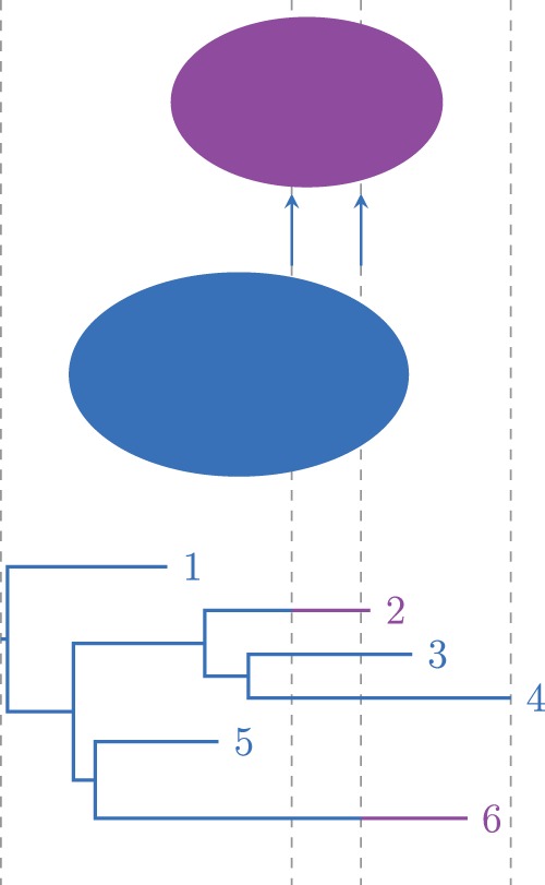
Multitype tree with two types. Tips 2 and 6 were sampled from the purple subpopulation, all others from the blue one. Two type-change events occur, both from blue to purple.

Here, we present a fully probabilistic approach for the joint reconstruction of phylogenies and epidemiological parameters, given structured host and/or pathogen populations, based on a multitype birth–death model. We test our approach through simulations and present two data analyses. First, we analyze the phylogeography of a global human influenza H3N2 virus data set, demonstrating how seasonal dynamics can be inferred simultaneously with the phylogeny and migration process. Second, the time-dependent transmission dynamics between and within HIV risk groups in the Latvian HIV epidemic are investigated.

Our method is general to both geographic and nongeographic (e.g., risk group) partitioning. We will use “subpopulation” to identify a group (geographic or otherwise) and type to identify the group membership of a sample; these terms are not meant to give preference to geographic or nongeographic situations.

The method is implemented as a package within the widely used Bayesian inference framework BEAST2 (Bouckaert et al. 2014), which makes it accessible to a wide audience. Our open source implementation is available at https://github.com/denisekuehnert/bdmm (last accessed April 15, 2016).

New Approaches

In this section, we introduce the multitype birth–death model. We combine a birth–death skyline (BDSKY) process (Stadler et al. 2013) on a population divided into a finite number d of discrete (typed) subpopulations with a “type-change” process among the subpopulations. The state of this continuous time Markov process comprised d random variables $N_1(t)\dots N_d(t)$ denoting the number of individuals in subpopulations $1\dots d$ at time t. In the context of infectious diseases, the population size N_i corresponds to the number of infected hosts present in subpopulation $i\in \{1\dots d\}$.

The Multitype Birth–Death Process

The multitype birth–death process is started with one infected individual in the subpopulation of type $i\in \{1\dots d\}$ at time t  =  0. Time increases from the past (where t = 0) to the present (at time T). In a time step $\Delta t$_, the process can undergo

1. A birth event, corresponding to transmission, so that another infected individual is created in subpopulation i:

   $$N_i(t+\Delta t)=N_i(t)+1,$$
2. A death event, corresponding to the recovery or removal of an infected individual in subpopulation i:

   $$N_i(t+\Delta t)=N_i(t)-1,$$

3. A sampling event, corresponding to the observation of an infected individual; if the removal probability r > 0, then the sampling event yields the removal of the individual with probability r (see (2))

4. A type-change event, indicating that an individual changes from subpopulation i to subpopulation $j\ne i$:

   $$N_i(t+\Delta t)=N_i(t)-1\text{\hspace{0.17em}\hspace{0.17em}and\hspace{0.17em}\hspace{0.17em}}{N}_j(t+\Delta t)=N_j(t)+1.$$
5. A birth event among demes, so that an infected individual in subpopulation i causes a new infected individual to arise in subpopulation j:

   $$N_i(t+\Delta t)=N_i(t)\text{\hspace{0.17em}and\hspace{0.17em}}{N}_j(t+\Delta t)=N_j(t)+1.$$

The process terminates when no infected individuals are left in any of the subpopulations.

The multitype birth–death process is an extension of the BDSKY process (Stadler et al. 2013) that allows the underlying population to be structured. Assume every sample is taken from one of d discrete subpopulations. Since subpopulations may have characteristics that influence the spread of a pathogen, the epidemic parameters may differ between subpopulations $i\in \{1\dots d\}$, see figure 2a for d = 2. As in Stadler et al. (2013), transmission events are modeled through births of new lineages, recovery or removal events are modeled as deaths, and sampling occurs either continuously through time determined by a sampling rate and/or through a contemporaneous sampling event at present (determined by a probability ρ_i of being sampled). For cases in which individuals are likely to continue transmitting to others after they were sampled, we include a removal probability r at which sampled individuals are removed from the infectious pool, as introduced by Gavryushkina et al. (2014). The birth, death, and sampling rates are allowed to change through time as piecewise constant rates. The overall time interval $[0,T]$ can be split into n intervals and each interval $k\in \{1\dots n\}$ is characterized by its rates ${\lambda }_{i,k},{\mu }_{i,k}$_, and ${\psi }_{i,k}$, where i denotes the current type and k the current interval. The type-change rates are assumed to be constant over time in our implementation, but from a mathematical perspective it is straightforward to also change these rates through time. The number n of time subdivisions has to be set a priori. The times at which changes occur may be inferred from the data though.

Fig. 2.

Examples of two-type applications of the multitype birth–death model. (a) In a classic phylogeographic setting, transmission can only occur within compartments I₁ and I₂, which are connected by type-change events at rates $m_{1,2}$ and $m_{2,1}$. The three-type version of this setup was used in the analysis of the Human Influenza H3N2 virus data set. (b) Alternatively, transmission events between subpopulations are possible instead of type-changes. This was employed for the analysis of the Latvian HIV data set. (c) A combination of (a) and (b) is also possible in which type changes and infections among types are allowed. This has been utilized in a previous study on Ebola virus, in which the time during which individuals are infected but not yet infectious (“exposed”) can be very long. Here, transmission events occur at rate λ_IE and originate in the infectious compartment (I), leading to a new exposed individual (E). Type-changes are only allowed from E to I, reflecting the progression of exposed individuals to the infectious phase at rate m_EI.

Hence, there are up to $d·n$ birth rates ${\lambda }_{1,1}\dots {\lambda }_{d,n},d·n$ death rates ${\mu }_{1,1}\dots {\mu }_{d,n}$ and $d·n$ sampling rates ${\psi }_{1,1}\dots {\psi }_{d,n}$. Individuals in subpopulation i move to subpopulation $j\in \{1\dots d\},j\ne i$, at type-change rate m_ij, thus we have up to $(d^2-d)$ type-change rates.

Figure 3 illustrates the notation under the multitype birth–death model with a two-type example and one type-change event at time z₁. As described above, the event is indicated by a node with in-degree one and out-degree one, at which the type of lineage (indicated by the color) changes.

Fig. 3.

Notation under the multitype birth–death model. Birth events are denoted by x_j, sampling events by y_j, and the one type-change event z₁.

The Multitype Birth–Death Likelihood

We now derive the likelihood of the multitype birth–death parameters $\mathit{\lambda },\mathit{\mu },\mathit{\psi },\mathit{r}$ and $\mathit{m}$ for a given tip-typed tree. This likelihood is obtained by considering the probability that an individual evolved as observed in the tree.

The Probability Density g that an Individual Evolved as Observed in the Tree

The probability density $g_{i,k}^e(t)$ denotes the probability that an individual with type $i\in \{1\dots d\}$ at time $t_{k-1}\le t<t_k$ has evolved between t and T as observed in the tree. We can evaluate $g_{i,k}^e(t)$ using the (backward in time) master equation

$$\begin{array}{l}-\frac{d}{dt}{g}_{i.k}^e(t)=-\left({\displaystyle \sum _{j=1}^d({\lambda }_{ij,k}+m_{ij})}+{\mu }_{i,k}+{\psi }_{i,k}\right)g_{i,k}^e(t)\\ +{\displaystyle \sum _{j=1}^d{m}_{ij}}{g}_{j,k}^e(t)+{\displaystyle \sum _{j=1}^d{\lambda }_{ij,k}}{p}_{j,k}(t)g_{i,k}^e(t)\\ +{\displaystyle \sum _{j=1}^d{\lambda }_{ij,k}}{p}_{i,k}(t)g_{j,k}^e(t),\left(1\right)\end{array}$$

with ${\lambda }_{ij,k}$ denoting the infection rate from type i to type j, ${\lambda }_{ii,k}$ denoting the infection rate within type i during interval k, and m_ii = 0 and initial conditions

$$g_{i,k}^e(t_e)=\{\begin{array}{ll}{\psi }_{i,k}(r+(1-r)p_{i,k}(t_e))& \text{\hspace{0.17em}if\hspace{0.17em}edge\hspace{0.17em}}e\text{\hspace{0.17em}is\hspace{0.17em}a\hspace{0.17em}serially\hspace{0.17em}sampled\hspace{0.17em}leaf},\\ {\psi }_{i,k}(1-r)g_{i,k}^{e_1}(t_e)& \text{\hspace{0.17em}if\hspace{0.17em}edge\hspace{0.17em}}e\text{\hspace{0.17em}is\hspace{0.17em}a\hspace{0.17em}sampled\hspace{0.17em}ancestor with descendant edge\hspace{0.17em}}{e}_1,\\ {\rho }_i& \text{\hspace{0.17em}if\hspace{0.17em}edge\hspace{0.17em}}e\text{\hspace{0.17em}is\hspace{0.17em}a\hspace{0.17em}contemporaneously\hspace{0.17em}sampled\hspace{0.17em}leaf\hspace{0.17em}at\hspace{0.17em}present},\\ {\displaystyle {\sum }_{j=1}^d{\lambda }_{ij,k}}\left[g_{i,k}^{e_1}(t_e)g_{j,k}^{e_2}(t_e)+g_{j,k}^{e_1}(t_e)g_{i,k}^{e_2}(t_e)\right]& \text{\hspace{0.17em}if\hspace{0.17em}edge\hspace{0.17em}}e\text{\hspace{0.17em}has\hspace{0.17em}two\hspace{0.17em}descendant\hspace{0.17em}edges\hspace{0.17em}}{e}_1,e_2.\end{array}$$

Starting at the most recent tip of a tree going backward in time, equation (1) results from considering the events that may occur during time step $\Delta t$:

$$\begin{array}{lll}{g}_{i,k}^e(t+\Delta t)=& \left(1-\left({\displaystyle {\sum }_{j=1}^d({\lambda }_{ij,k}+m_{ij})}+{\mu }_{i,k}+{\psi }_{i,k}\right)\Delta t\right)g_{i,k}^e(t)& (\text{nothing\hspace{0.17em}happens\hspace{0.17em}})\\ & & \\ & +{\displaystyle {\sum }_{j=1}^d{\lambda }_{ij,k}}{p}_{j,k}(t)g_{i,k}^e(t)& (\text{\hspace{0.17em}a\hspace{0.17em}birth\hspace{0.17em}of\hspace{0.17em}type\hspace{0.17em}}j\text{\hspace{0.17em}happens},\text{\hspace{0.17em}lineage\hspace{0.17em}}j\text{\hspace{0.17em}produces\hspace{0.17em}}\text{no\hspace{0.17em}samples\hspace{0.17em}in\hspace{0.17em}}t)\\ & +{\displaystyle {\sum }_{j=1}^d{\lambda }_{ij,k}}{p}_{i,k}(t)g_{j,k}^e(t)& (\text{a\hspace{0.17em}birth\hspace{0.17em}of\hspace{0.17em}type\hspace{0.17em}}j\text{\hspace{0.17em}happens},\text{\hspace{0.17em}lineage\hspace{0.17em}}i\text{\hspace{0.17em}produces}\text{no\hspace{0.17em}samples\hspace{0.17em}in\hspace{0.17em}}t)\\ & +O(\Delta t^2)& (\text{more\hspace{0.17em}than\hspace{0.17em}one\hspace{0.17em}event\hspace{0.17em}in\hspace{0.17em}}\Delta t)\end{array}$$

Rearrangement of this equation and letting $\Delta t\to 0$ yields equation (1), with $g_{i,0}(0)$ denoting the likelihood given the individual at time 0 has type i.

The last two summed terms in the equation for g^e give the probability (during $\Delta t$) that an infection event from i to j left no sampled descendants, while the sister lineage survived and gave rise to the observed subtree, with one term for i surviving and one term for j surviving.

The Probability p of Having No Sampled Descendants

To compute the probability densities $g_{i,k}^e(t)$, we need to calculate the probability $p_{i,k}(t)$ of an individual with type $i\in \{1\dots d\}$ at time $t_{k-1}\le t<t_k$ to have no sampled descendants. This probability can be calculated by the (backward in time) master equation

$$\begin{array}{l}-\frac{d}{dt}{p}_{i,k}(t)=-\left({\displaystyle \sum _{j=1}^d({\lambda }_{ij,k}+m_{ij})}+{\mu }_{i,k}+{\psi }_{i,k}\right)p_{i,k}(t)+{\displaystyle \sum _{j=1}^d{\lambda }_{ij,k}}{p}_{i,k}(t)p_{j,k}(t)+{\displaystyle \sum _{j=1}^d{m}_{ij}}{p}_{j,k}(t)+{\mu }_{i,k}\end{array}$$ (2)

with initial condition

$$p_{i,k}(T)=1\forall i,j\in \{1\dots d\},k\in \{1\dots n\}.$$

This master equation also follows from considering the events that may occur during time step $\Delta t$:

$$\begin{array}{lll}{p}_{i,k}(t+\Delta t)=& \left(1-\left({\displaystyle {\sum }_{j=1}^d({\lambda }_{ij,k}+m_{ij})}+{\mu }_{i,k}+{\psi }_{i,k}\right)\Delta t\right)p_{i,k}(t)& \left(\text{nothing happens}\right)\\ & +{\displaystyle {\sum }_{j=1}^d\Delta t{\lambda }_{ij,k}}{p}_{i,k}(t)p_{j,k}(t)& \left(\text{a birth event happens}\right)\\ & +{\displaystyle {\sum }_{j=1}^d{m}_{ij}}\Delta t{p}_{j,k}(t)& \left(\text{a type}-\text{change event to subpopulation\hspace{0.17em}}j\right)\\ & +{\mu }_{i,k}\Delta t& \left(\text{a death event without sampling}\right)\\ & +O(\Delta t^2)& (\text{more than one event in }\Delta \text{t})\end{array}$$

Again, equation (2) is obtained by letting $\Delta t\to 0$.

The likelihood is derived analogously to equation (2.3) in Stadler and Bonhoeffer (2013), which is based on ideas from (Maddison et al. 2007). Our notation here is based on previous work (Stadler et al. 2013), but for comparison, the probabilities $p_{i,k}(t)$ and $g_{i,k}^e$ relate to E and D in Maddison et al. (2007) and Stadler and Bonhoeffer (2013), respectively.

The Probability Density f of a Tree $\mathcal{T}$

The probability density of a tree with the lineage belonging to the root having type i at time t = 0 is the product of the probability density that the individual evolved as observed in the tree and the probability that the individual is in type i.

Hence, the probability density f of a tree $\mathcal{T}$ under the multitype birth–death model is

$$f(\mathcal{T}|\mathit{\lambda },\mathit{\mu },\mathit{\psi },\mathit{m},t)={\displaystyle \sum _{\mathit{i}=1}^{\mathit{d}}{h}_{\mathit{i}}{\mathit{g}}_{\mathit{i},0}^{\mathit{e}}(0)}.$$

The probability $h_i$ that an individual is with type i can be chosen to be equal for each type, that is, $h_i=\frac{1}{d}$ or the equilibrium frequency for each type can be calculated, as suggested by Stadler and Bonhoeffer (2013). However, this implicitly assumes that the birth and death rates are in equilibrium as well. Since the multitype birth–death model developed here allows birth and death rates to change over time, this is not always the case. Instead, we use the fact that the Bayesian framework allows $h_i$ to be treated as a random variable and to be estimated from the data.

Inference under the Multitype Birth–Death Model

We sample from the posterior distribution of the evolutionary and epidemiological parameters using a Markov chain Monte Carlo algorithm within the Bayesian inference framework BEAST2.

Inference on Tip-Typed Trees

In the likelihood stated above, we integrate over the type-change process along the tree, as was previously described by Stadler and Bonhoeffer (2013). This means that the only phylogeographic information that is annotated with the tree is the types at the leaves. We will refer to such trees as tip-typed trees. In the following, we refer to this as the “integrated-likelihood” multitype birth–death model, which is useful, for example, when the considered subpopulations are distinguished by characteristics that allow infections in one subpopulation being caused by another (e.g., risk groups, fig. 2b) or when subpopulations are defined as epidemiological compartments (e.g., as exposed and infected compartments, fig. 2c).

Inference of Multitype Trees

When the timing of and the subpopulations involved in type-change events are important, we infer multitype trees, which are timed phylogenetic trees in which lineages are associated with a type (Vaughan et al. 2014). Thus we sample type-change histories jointly with the evolutionary and epidemiological parameters. This is often useful in classic phylogeographic analyses, in which samples were obtained from distinct geographical subpopulations and infected individuals can move among the discrete subpopulations (fig. 2a depicts the two-type scenario).

This multitype birth–death model employs a multitype tree structure and operators introduced by Vaughan et al. (2014). The implementation of changes along branches is realized by first annotating each leaf node with a type. Then, the information of any change of type (migration) is stored in arrays associated with the tree nodes.

When inferring multitype trees, the integration over the type-change process is unnecessary. We define η_i,j = 1 for i ≠ j, and for i=j. Hence equation (1) is replaced by

$$-\frac{\text{d}}{\text{d}t}{g}_{i.k}^e(t)=-\left({\displaystyle \sum _{j=1}^d({\lambda }_{ij,k}+m_{ij})}+{\mu }_{i,k}+{\psi }_{i,k}\right)g_{i,k}^e(t)+{\displaystyle \sum _{j=1}^d{\eta }_{ij}{\lambda }_{ij,k}}{p}_{j,k}(t)g_{i,k}^e(t)$$

with initial conditions

$$g_{i,k}^e(t_e)=\{\begin{array}{ll}{\psi }_{i,k}(r+(1-r)p_{i,k}(t_e))& \text{\hspace{0.17em}if\hspace{0.17em}edge\hspace{0.17em}}e\text{\hspace{0.17em}is\hspace{0.17em}a\hspace{0.17em}serially\hspace{0.17em}sampled\hspace{0.17em}leaf},\\ {\psi }_{i,k}(1-r)g_{i,k}^{e_1}(t_e)& \text{\hspace{0.17em}if\hspace{0.17em}edge\hspace{0.17em}}e\text{\hspace{0.17em}is\hspace{0.17em}a\hspace{0.17em}sampled\hspace{0.17em}ancestor\hspace{0.17em} with descendant edge\hspace{0.17em}}{e}_1,\\ {\rho }_i& \text{\hspace{0.17em}if\hspace{0.17em}edge\hspace{0.17em}}e\text{\hspace{0.17em}is\hspace{0.17em}a\hspace{0.17em}contempor}.\text{\hspace{0.17em}sampled\hspace{0.17em}leaf\hspace{0.17em}at\hspace{0.17em}present},\\ m_{ij}{g}_{j,k}^{e_1}(t_e)+{\lambda }_{ij}{g}_{j,k}^{e_1}{p}_{ik}& \text{\hspace{0.17em}if\hspace{0.17em}edge\hspace{0.17em}}e\text{\hspace{0.17em}has\hspace{0.17em}one\hspace{0.17em}descendant\hspace{0.17em}edge\hspace{0.17em}}{e}_1\text{with\hspace{0.17em}type\hspace{0.17em}}j,\\ {\displaystyle {\lambda }_{ij,k}}{g}_{i,k}^{e_1}{g}_{j,k}^{e_2}& \text{\hspace{0.17em}if\hspace{0.17em}edge\hspace{0.17em}}e\text{\hspace{0.17em}has\hspace{0.17em}two\hspace{0.17em}descendant\hspace{0.17em}edges\hspace{0.17em}}{e}_1\text{\hspace{0.17em}with type i and\hspace{0.17em}}{e}_2\text{with type j}.\end{array}$$

Because of the implementation of the tree structure, our current implementation of the multitype model does not allow birth events among demes (i.e. λ_ij = 0 for i ≠ j).

Parameterization of the Multitype Birth Death Model

The multitype birth–death model parameterizes the within-type effective reproduction number $R_{i,k}:=R_{ii,k}$ and the between-type effective reproduction number $R_{ij,k}$ (with $i\ne j$) for all $i,j\in \{1\dots d\}$ and $k\in \{1\dots n\}$ as follows:

$$R_{ij,k}=\frac{{\lambda }_{ij,k}}{{\mu }_{i,k}+r{\psi }_{i,k}}.$$

The duration of infection ${\tau }_{i,k}=\frac{1}{{\delta }_{i,k}}$ in subpopulation $i\in \{1\dots d\}$ and interval $k\in \{1\dots n\}$ is determined by the rate of becoming noninfectious,

$${\delta }_{i,k}={\mu }_{i,k}+r{\psi }_{i,k},$$

and the probability of an individual to be (serially) sampled is

$$s_{i,k}=\frac{{\psi }_{i,k}}{{\mu }_{i,k}+{\psi }_{i,k}}.$$

When the type-change rates are nonzero, no analytical solutions are available for the master equations, so that numerical integration is required to determine the solutions. They are solved using a classic Runge–Kutta integrator. Both implementations were validated by comparing the sampled tree distributions to direct simulation with MASTER (Vaughan and Drummond 2013), see figure 4.

Fig. 4.

Validation of tree height distribution. The tree height distributions of four-tip trees with two leaves of each type sampled from the multitype birth–death distribution using our implementation of the described Markov chain Monte Carlo (MCMC) algorithm (black lines) with those generated via direct simulation (gray lines). For (a) the stopping criterium for the simulations was the simulation time (set to 8), which implies that the origin of the resulting epidemic (t_m in fig. 3) in the MCMC is also 8. In (b) t_m was allowed to vary, that is, it was sampled jointly with the tree.

Results

Simulations

In two scenarios (with and without piecewise constant rate change), the re-estimation of the effective reproduction number, the rate of becoming noninfectious, and the type-change rates are assessed. Each of the 120 simulated 100-taxon alignments is analyzed with the sampling proportion fixed to the true value. The results for the three-type-simulations are summarized in tables 1 and 2 for multitype trees and tables 3 and 4 for tip-typed trees from the integrated-likelihood analyses. The results for the two-type-simulations are summarized in tables 5–8. In the description of each table, we report the number of simulation replicates that had an effective sample size larger or equal to 200 for each parameter.

Table 1.

Simulation Results from Multitype Birth–Death Three-Type Scenario 1: Constant Rates.

	Truth	Median	Relative	Relative	Relative	95% HPD
			Error	Bias	HPD Width	Accuracy
$R_{{\text{e}}_1}$	1.333	1.298	0.138	−0.027	0.653	97.000
$R_{{\text{e}}_2}$	1.500	1.375	0.205	−0.083	0.926	90.000
$R_{{\text{e}}_3}$	1.500	1.520	0.210	0.014	1.172	96.000
δ1	0.300	0.307	0.193	0.023	1.188	94.000
δ2	0.200	0.224	0.249	0.122	1.712	95.000
δ3	0.200	0.200	0.193	−0.002	1.330	95.000
$m_{1,2}$	0.030	0.034	0.378	0.132	2.375	96.000
$m_{1,3}$	0.010	0.016	0.725	0.585	4.186	99.000
$m_{2,1}$	0.030	0.033	0.379	0.089	2.793	98.000
$m_{2,3}$	0.010	0.017	0.796	0.686	5.134	100.000
$m_{3,1}$	0.010	0.021	1.139	1.123	7.123	100.000
$m_{3,2}$	0.010	0.023	1.326	1.309	7.393	98.000

Note.—HPD, highest posterior density. Posterior parameter estimates and accuracy obtained from simulated alignments with 100 taxa. For each parameter, the median over all medians (1 for each alignment)/errors/biases/HPD widths/HPD accuracies is provided. Out of 120 simulation replicates the 110 for which all parameters yielded a minimum effective sample size (ESS) of 200) are included here.

Table 2.

Simulation Results from Multitype Birth–Death Three-Type Scenario 2: R_e Rate Change.

Parameter	Truth	Median	Relative	Relative	Relative	95% HPD
			Error	Bias	HPD Width	Accuracy
$R_{{\text{e}}_{1,1}}$	1.333	1.235	0.215	−0.073	0.745	87.000
$R_{{\text{e}}_{1,2}}$	1.167	1.110	0.222	−0.049	0.790	85.000
$R_{{\text{e}}_{2,1}}$	1.500	1.347	0.379	−0.102	1.186	84.000
$R_{e_{2,2}}$	1.250	1.185	0.241	−0.052	1.079	85.000
$R_{e_{3,1}}$	1.500	1.208	0.315	−0.195	1.562	94.000
$R_{e_{3,2}}$	1.250	1.248	0.252	−0.002	1.192	90.000
δ1	0.300	0.492	0.828	0.639	1.823	83.000
δ2	0.200	0.291	0.626	0.454	1.554	86.000
δ3	0.200	0.202	0.244	0.009	1.155	87.000
$m_{1,2}$	0.030	0.031	0.368	0.018	1.978	88.000
$m_{1,3}$	0.010	0.014	0.608	0.437	3.763	97.000
$m_{2,1}$	0.030	0.030	0.456	0.006	2.067	79.000
$m_{2,3}$	0.010	0.015	0.594	0.449	3.789	98.000
$m_{3,1}$	0.010	0.017	0.790	0.727	5.140	98.000
$m_{3,2}$	0.010	0.019	0.929	0.857	5.159	95.000

Note.—HPD, highest posterior density. Posterior parameter estimates and accuracy obtained from simulated alignments with 100 taxa. For each parameter, the median over all medians (1 for each alignment)/errors/biases/HPD widths/HPD accuracies is provided. Out of 120 simulation replicates, the 99 for which all parameters yielded a minimum effective sample size (ESS) of 200 are included here. The effective reproduction number $R_{e_{i,k}}$ refers to subpopulation i in time interval k.

Table 3.

Simulation Results from Integrated-Likelihood Multitype Birth–Death Three-Type Scenario 1: Constant Rates.

Parameter	Truth	Median	Relative	Relative	Relative	95% HPD
			Error	Bias	HPD Width	Accuracy
$R_{e_1}$	1.333	1.302	0.139	−0.023	0.751	99.000
$R_{e_2}$	1.500	1.380	0.197	−0.080	1.026	94.000
$R_{e_3}$	1.500	1.540	0.201	0.027	1.242	98.000
δ1	0.300	0.301	0.174	0.002	1.253	99.000
δ2	0.200	0.218	0.220	0.091	1.735	96.000
δ3	0.200	0.192	0.170	−0.042	1.241	98.000
$m_{1,2}$	0.030	0.041	0.558	0.368	3.330	97.000
$m_{1,3}$	0.010	0.018	0.862	0.749	5.320	98.000
$m_{2,1}$	0.030	0.039	0.495	0.298	3.801	100.000
$m_{2,3}$	0.010	0.019	0.928	0.858	6.349	100.000
$m_{3,1}$	0.010	0.025	1.482	1.467	8.860	100.000
$m_{3,2}$	0.010	0.026	1.670	1.653	9.067	99.000

Note.—HPD, highest posterior density. Posterior parameter estimates and accuracy obtained from simulated alignments with 100 taxa. For each parameter, the median over all medians (1 for each alignment)/errors/biases/HPD widths/HPD accuracies is provided. All 120 simulation replicates yielded a minimum effective sample size (ESS) of 200 and are included here.

Table 4.

Simulation Results from Integrated-Likelihood Multitype Birth–Death Three-Type Scenario 2: R_e Rate Change.

Parameter	Truth	Median	Relative	Relative	Relative	95% HPD
			Error	Bias	HPD Width	Accuracy
$R_{e_{1,1}}$	1.333	1.272	0.203	−0.046	0.906	96.000
$R_{e_{1,2}}$	1.167	1.164	0.177	−0.003	0.911	94.000
$R_{e_{2,1}}$	1.500	1.241	0.313	−0.173	1.309	94.000
$R_{e_{2,2}}$	1.250	1.154	0.219	−0.077	1.246	95.000
$R_{e_{3,1}}$	1.500	1.193	0.321	−0.204	1.605	97.000
$R_{e_{3,2}}$	1.250	1.278	0.226	0.022	1.438	98.000
δ1	0.300	0.289	0.177	−0.037	1.046	95.000
δ2	0.200	0.208	0.204	0.040	1.627	99.000
δ3	0.200	0.185	0.207	−0.074	1.138	94.000
$m_{1,2}$	0.030	0.040	0.512	0.316	3.086	98.000
$m_{1,3}$	0.010	0.016	0.662	0.569	4.372	100.000
$m_{2,1}$	0.030	0.041	0.563	0.361	4.104	99.000
$m_{2,3}$	0.010	0.019	0.992	0.946	6.884	100.000
$m_{3,1}$	0.010	0.026	1.602	1.587	9.970	100.000
$m_{3,2}$	0.010	0.027	1.700	1.689	9.620	99.000

Note.—HPD, highest posterior density. Posterior parameter estimates and accuracy obtained from simulated alignments with 100 taxa. For each parameter, the median over all medians (1 for each alignment)/errors/biases/HPD widths/HPD accuracies is provided. Out of 120 simulation replicates, the 116 for which all parameters yielded a minimum effective sample size (ESS) of 200 are included here. The effective reproduction number $R_{e_{i,k}}$ refers to subpopulation i in time interval k.

Table 5.

Simulation Results from Multitype Birth–Death Two-Type Scenario 1: Constant Rates.

Parameter	Truth	Median	Relative	Relative	Relative	95% HPD
			Error	Bias	HPD Width	Accuracy
$R_{e_1}$	1.333	1.350	0.082	0.013	0.395	98.000
$R_{e_2}$	1.650	1.655	0.156	0.003	0.857	96.000
δ1	0.300	0.297	0.132	−0.010	0.661	94.000
δ2	0.200	0.203	0.184	0.015	1.002	97.000
$m_{1,2}$	0.010	0.013	0.406	0.292	2.148	97.000
$m_{2,1}$	0.030	0.035	0.410	0.172	2.433	94.000

Note.—HPD, highest posterior density. Posterior parameter estimates and accuracy obtained from simulated alignments with 100 taxa. For each parameter, the median over all medians (1 for each alignment)/errors/biases/HPD widths/HPD accuracies is provided. Out of 120 simulation replicates, the 111 for which all parameters yielded a minimum effective sample size (ESS) of 200 are included here.

Table 6.

Simulation Results from Multitype Birth–Death Two-Type Scenario 2: R_e Rate Change.

Parameter	Truth	Median	Relative	Relative	Relative	95% HPD
			Error	Bias	HPD Width	Accuracy
$R_{e_{1,1}}$	1.333	1.283	0.128	−0.038	0.548	93.000
$R_{e_{1,2}}$	1.167	1.175	0.071	0.007	0.323	90.000
$R_{e_{2,1}}$	1.650	1.193	0.371	−0.277	1.393	93.000
$R_{e_{2,2}}$	1.250	1.177	0.178	−0.058	0.741	87.000
δ1	0.300	0.297	0.109	−0.011	0.497	89.000
δ2	0.200	0.215	0.227	0.077	1.043	93.000
s1	0.050	0.050	0.000	0.000	0.000	0.000
s2	0.150	0.150	0.000	0.000	0.000	0.000
$m_{1,2}$	0.010	0.011	0.298	0.147	1.506	94.000
$m_{2,1}$	0.030	0.030	0.345	0.003	2.003	95.000

Note.—HPD, highest posterior density. Posterior parameter estimates and accuracy obtained from simulated alignments with 100 taxa. For each parameter, the median over all medians (1 for each alignment)/errors/biases/HPD widths/HPD accuracies is provided. Out of 120 simulation replicates, the 102 for which all parameters yielded a minimum effective sample size (ESS) of 200 are included here. The effective reproduction number $R_{e_{i,k}}$ refers to subpopulation i in time interval k.

Table 7.

Simulation Results from Integrated-Likelihood Multitype Birth–Death Two-Type Scenario 1: Constant Rates.

Parameter	Truth	Median	Relative	Relative	Relative	95% HPD
			Error	Bias	HPD Width	Accuracy
$R_{e_1}$	1.333	1.361	0.077	0.021	0.410	97.000
$R_{e_2}$	1.650	1.633	0.156	−0.010	0.898	97.000
δ1	0.300	0.293	0.130	−0.023	0.653	94.000
δ2	0.200	0.204	0.189	0.020	1.063	98.000
$m_{1,2}$	0.010	0.014	0.521	0.412	2.547	97.000
$m_{2,1}$	0.030	0.037	0.486	0.244	2.941	94.000

Note.—HPD, highest posterior density. Posterior parameter estimates and accuracy obtained from simulated alignments with 100 taxa. For each parameter, the median over all medians (1 for each alignment)/errors/biases/HPD widths/HPD accuracies is provided. Out of 120 simulation replicates, the 117 for which all parameters yielded a minimum effective sample size (ESS) of 200 are included here.

Table 8.

Simulation Results from Integrated-Likelihood Multitype Birth–Death Two-Type Scenario 2: R_e Rate Change.

Parameter	Truth	Median	Relative	Relative	Relative	95% HPD
			Error	Bias	HPD Width	Accuracy
$R_{e_{1,1}}$	1.333	1.276	0.133	−0.043	0.586	97.000
$R_{e_{1,2}}$	1.167	1.179	0.076	0.011	0.376	95.000
$R_{e_{2,1}}$	1.650	1.154	0.386	−0.300	1.253	93.000
$R_{e_{2,2}}$	1.250	1.208	0.174	−0.034	0.913	94.000
δ1	0.300	0.295	0.109	−0.015	0.556	92.000
δ2	0.200	0.207	0.194	0.033	1.092	97.000
$m_{1,2}$	0.010	0.014	0.464	0.366	2.317	95.000
$m_{2,1}$	0.030	0.041	0.536	0.349	3.267	99.000

Note.—HPD, highest posterior density. Posterior parameter estimates and accuracy obtained from simulated alignments with 100 taxa. For each parameter, the median over all medians (1 for each alignment)/errors/biases/HPD widths/HPD accuracies is provided. All 120 simulation replicates yielded a minimum effective sample size (ESS) of 200 and are included here. The effective reproduction number $R_{e_{i,k}}$ refers to subpopulation i in time interval k.

Accuracy is always above or equal to 90% in scenario 1. In scenario 2, accuracy decreases in some cases, with the lowest accuracy at 79%. Our results underline the importance of the sampling process: In both scenarios, the largest relative errors occur for the parameters related to type 3, which in 62% of the simulations is the latest to be sampled (when comparing the time of the first sample per type). That is, the respective subepidemics of type 3 commence later than the other subepidemics. Since the simulations are stopped when a total of 100 samples have been obtained, the data contain the least information about the subepidemic that started last (it might even have started just before the end of the sampling period).

Analyzing the two- and three-type simulations using the BDSKY model (Stadler et al. 2013) yields average estimates of R_e and δ, which are close to the parameter values under which the multitype data sets where simulated (table 9). Tables 1, 3, and 9(c); tables 2, 8, and 9(d); tables 5, 7 and 9(a); and tables 6, 8 and 9(b) refer to the same set of simulations, respectively.

Table 9.

Simulation Results from Nonstructured BDSKY Analysis of Two- And Three-Type Simulations.

	BDMM Simulation			BDSKY Average
(a)		Type 1	Type 2	Median	Relative HPD Width
$R_{e_1}$		1.333	1.650	1.524	0.459
δ		0.300	0.200	0.217	0.153
(b)		Type 1	Type 2	Median	Relative HPD Width
$R_{e_1}$		1.333	1.650	1.445	0.550
$R_{e_2}$		1.167	1.250	1.251	0.420
δ		0.300	0.200	0.194	0.056
(c)	Type 1	Type 2	Type 3	Median	Relative HPD Width
$R_{e_1}$	1.333	1.500	1.500	1.496	0.461
δ	0.300	0.200	0.200	0.213	0.131
(d)	Type 1	Type 2	Type 3	Median	Relative HPD Width
$R_{e_1}$	1.333	1.500	1.500	1.436	0.552
$R_{e_2}$	1.167	1.250	1.250	1.225	0.707
δ	0.300	0.200	0.200	0.206	0.094

Note.—HPD, highest posterior density. Posterior parameter estimates obtained from simulated alignments with 100 taxa. The simulated data sets referred to in tables 5 and 6 for two types without (a) and with (b) a change in R_e and tables 1 and 2 for three types without (c) and with (d) a change in R_e were used. For each parameter, the true parameter per type is provided together with the estimated median over all medians (1 for each alignment) and HPD widths.

Global Human Influenza H3N2

Given the genetic information from 175 globally sampled sequences together with the dates of sampling and the subpopulation each sample was obtained from, the multitype birth–death model recovers the typical seasonal dynamics of global human influenza H3N2. Figure 5 shows the estimated effective reproduction numbers R_e for each subpopulation and half-year. In the tropics, R_e always stays very close to the epidemic threshold at one. In the temperate regions, the median estimate of R_e is always above one in winter and below one in summer, with most of the 95% highest posterior density intervals not including the threshold, one.

Fig. 5.

Spatial H3N2 influenza analysis: effective reproduction numbers through time. The estimated median effective reproduction numbers for each half year in the (a) northern, (b) tropical, and (c) southern region with 95% highest posterior density (HPD) intervals (whiskers).

We estimate a total of 53 migration events (median) in the three-year period covered by this sample, the largest proportion of which (43%) occurred from the tropics to the northern region (table 10). In fact, the rate at which a lineage migrates from the tropics to the north $m_{\text{T,N}}$ is significantly larger than the one from the tropics to the south $m_{\text{T,S}}$ (BF = 19,000). We also see more clustering among southern samples than among northern samples, which is not surprising since the southern samples are from Australia and New Zealand only, while the northern subpopulation covers a larger area, including locations in Europe as well as the United States. Likewise, $m_{\text{T,N}}$ is significantly larger than $m_{\text{N,T}}$, which is the rate corresponding to the reverse direction, north to tropics (BF = 19).

Table 10.

Spatial H3N2 Influenza Results.

Parameter	Median	95% HPD Lower	95% HPD Upper
t	2.950	2.795	3.160
δ	97.993	88.051	108.307
sN	8.22×10−4	4.51×10−4	12.72×10−4
sT	5.31×10−4	3.23×10−4	7.85×10−4
sS	8.67×10−4	4.51×10−4	13.92×10−4
$m_{N,T}$	0.478	0.076	1.170
$c_{N,T}$	8	1	18
$m_{N,S}$	0.140	0.019	0.373
$c_{N,S}$	1	0	4
$m_{T,N}$	1.628	0.410	3.885
$c_{T,N}$	23	10	39
$m_{T,S}$	0.151	0.042	0.313
$c_{T,S}$	8	4	11
$m_{S,N}$	0.706	0.069	1.930
$c_{S,N}$	8	0	17
$m_{S,T}$	0.466	0.065	1.198
$c_{S,T}$	5	0	11

Note.—HPD, highest posterior density. Posterior parameter estimates of H3N2 analysis. Median posterior estimates and 95% HPD intervals for the tree height t, the rate to become noninfectious δ, the sampling proportion in the north (s_N), tropics (s_T), and south (s_S), and the migration rates m_ij and estimated numbers of migration events c_ij from subpopulation i to j for $i,j\in \left\{\text{N,T,S}\right\}$.

The maximum sampled posterior tree (fig. 6a) as well as the posterior probability distribution of the root type (fig. 6b) place the root of the tree in the tropics, which is consistent with the hypothesis that the tropical regions are the source of seasonal influenza epidemics (Rambaut et al. 2008).

Fig. 6.

Spatial H3N2 influenza posterior phylogeny. (a) Maximum sampled posterior multitype tree and (b) the posterior root type probabilities.

HIV in Latvia

The transmission dynamics estimated from both genetic regions, V3 and p17, generally agree with one another (fig. 7 and table 12).

Fig. 7.

Risk group analysis of Latvian HIV. The effective reproduction number estimates resulting from the analysis of the p17 and the V3 region. For each of the three transmission periods, median estimates (dots) are plotted with 95% highest posterior density (HPD) intervals (whiskers) for transmission within the HET and IDU risk groups and between risk groups (HET to IDU, IDU to HET). The prior distribution employed for each effective reproduction number is plotted in gray.

Table 12.

Risk Group Analysis of Latvian HIV.

	V3			p17
Parameter	Median	95% HPD lower	95% HPD upper	Median	95% HPD lower	95% HPD upper
t	8.768	7.733	10.079	8.657	7.594	10.699
tm	9.320	8.167	11.080	9.455	7.785	13.968
δ	0.441	0.326	0.569	0.457	0.337	0.593
μM	0.005	0.003	0.006	0.003	0.002	0.004
μS	0.825	0.660	1.006	0.532	0.321	0.743
$s_{HE{T}_1}$	0.068	0.021	0.131	0.066	0.020	0.128
$s_{HE{T}_2}$	0.038	0.008	0.084	0.043	0.009	0.092
$s_{HE{T}_3}$	0.035	0.014	0.066	0.043	0.017	0.079
$s_{HE{T}_4}$	0.057	0.019	0.108	0.054	0.018	0.105
$s_{ID{U}_1}$	0.051	0.021	0.091	0.059	0.024	0.106
$s_{ID{U}_2}$	0.236	0.146	0.336	0.255	0.161	0.358
$s_{ID{U}_3}$	0.003	0.001	0.007	0.003	0.001	0.006
$s_{ID{U}_4}$	0.043	0.013	0.084	0.057	0.019	0.109

Note.—HPD, highest posterior density. The median posterior parameter estimates and 95% HPD intervals for the tree height t, the origin t_m, the rate to become noninfectious δ, the mean and standard deviation of the substitution rate μ_M, μ_S, and the sampling proportions per sampling period in each of the two risk groups $s_{{\text{HET}}_i}$ and $s_{{\text{IDU}}_i}$ for $i\in \left\{\mathrm{1..4}\right\}$. Transmission rates are shown in figure 7.

In the first transmission interval, before 1998, the estimates of the effective reproduction number within the subpopulations mainly reflect the prior distribution, which is plotted in gray (fig. 7). However, between risk groups, there is significantly more transmission from injecting drug user (IDU) to heterosexual (HET) than vice versa (Bayes factor BF = 5.5 for p17 and BF = 13.4 for V3).

Our results suggest a drastic change in transmission dynamics in the second interval, between 1997 and 2002. During that time, there was a large increase in transmissions within the IDU risk group. We estimate medians $R_{{\text{IDU}}_2}=4.9$ and $R_{{\text{IDU}}_{\text{2}}}=5.3$ for V3 and p17, respectively.

In the final interval, from 2002 to the time of the latest sample in 2005, all median reproduction number estimates are below one. This agrees with the epidemic peak observed in 2001 and a decline in new transmissions thereafter (Graw et al. 2012).

Figure 8 shows the maximum clade credibility trees estimated from (a) the V3 region and (b) the p17 region and depicts the periods of sampling $s_1\dots s_4$ for which piecewise constant sampling proportions were estimated. Our results suggest that in the first half of the year 2001 (sampling period s₂), the sampling proportion within the IDU risk group was significantly higher than in any of the other sampling periods and also higher than within the HET risk group at any time (table 12).

Fig. 8.

Risk group analysis of Latvian HIV: reconstructed phylogenies and sampling periods. The posterior maximum clade credibility trees for (a) the V3 and (b) the p17 region. The dotted lines indicate the four sampling regions $s_1,\dots s_4$ that are used to account for changes in sampling effort through time and between risk groups.

Discussion

This article introduces a Bayesian multitype birth–death model as a model for phylodynamic analysis of serially sampled sequence data from structured populations.

Within the three-way grouping of phylogeographic methods into comparative, spatial diffusion and population genetic approaches (Bloomquist et al. 2010), the multitype birth–death model belongs to the population genetic approaches. Many extensions of population genetic and diffusion approaches can be integrated here as well, for example, incorporation of hidden/nonsampled subpopulations (Ewing and Rodrigo 2006) or time-dependent type-change rates. In recent years, a number of powerful phylogeographic models have been developed, including models of wavefront velocity (Pybus et al. 2012) and models for the inference of viral cross-species transmission history (Faria et al. 2013).

The multitype birth–death model incorporates type-change events between discrete subpopulations, modeled by a type-change rate matrix, and allows for transmission events within as well as among subpopulations. Applied to viral transmission dynamics, birth and death/sampling events relate to infection and recovery, as in previous work (Kühnert et al. 2013; Stadler et al. 2013). Others have previously developed similar models in the context of speciation and extinction (Maddison et al. 2007; FitzJohn et al. 2009; Goldberg and Igić 2012; Magnuson-Ford and Otto 2012). They have focused on contemporaneously sampled data sets with restrictions on the model parameters that are given in Stadler and Bonhoeffer (2013). This model differs from the two-type maximum-likelihood approach (with serial sampling) introduced by Stadler and Bonhoeffer (2013) in that it allows the transmission parameters to change through time (in a piecewise constant fashion) and can handle more than two subpopulations and sampled ancestors (Gavryushkina et al. 2014). Furthermore, the model introduced here is implemented in a Bayesian framework, such that the type-change dynamics can be inferred jointly with the evolutionary parameters, and the phylogeny.

In phylogeographic methods that allow the joint estimation of the phylogeny and phylogeographic parameters of interest, population structure can either be regarded as independent from the population dynamics or be integrated in the population model. The assumption that the migration and diversification processes are conditionally independent led to a range of popular “discrete trait analysis” models, most of which are extensions or variations of a model published by Lemey et al. (2009). These conditionally independent processes ignore the interaction between population sizes and migration in shaping the sample genealogy, assuming that the migration process is independent of the subpopulation characteristics. Modeling migration as an independent diffusion process makes it feasible to analyze large data sets sampled from several distinct subpopulations. However, epidemiological characteristics can differ among subpopulations, leading to a dependence between the migration process and the tree-generating process. Ignoring this dependence may result in a loss of power, since the times between coalescence/migration events contain information about the migration process and may lead to false estimates that may be well supported nevertheless. In fact, Maio et al. (2015) showed that such discrete trait analysis may be fundamentally biased. Therefore, models that incorporate the migration dynamics into the tree-generating process are important.

The structured coalescent process (Hudson 1990; Notohara 1990) is a well-known example of a nonindependent model and has been implemented for phylogenetic analysis of structured phylogenetic data (Beerli and Felsenstein 1999, 2001; Anderson et al. 2005; Beerli and Palczewski 2010; Vaughan et al. 2014). However, the coalescent does not well approximate the early stage of an epidemic, which is typically driven by stochastic exponential population growth (Stadler et al. 2015). Therefore, we use the birth–death model, which has also been extended to allow migration among discrete subpopulations (Jones 2011; Stadler and Bonhoeffer 2013).

All phylogeographic methods struggle when the data are uninformative for one or more of the populations. For example, if the phylogeographic tree does not contain any branching events that occurred within one of the subpopulations, there is little information about the effective population size or the birth rate (Ewing et al. 2004). In such cases, the posterior estimate of the respective parameters will be dominated by the prior distribution. When designing phylogeographic studies researchers should keep in mind that any method will suffer from insufficient or biased sampling.

The simulation study showed that the multitype birth–death model recovers the epidemiological parameters and type-change rates well in epidemics connecting two or three distinct subpopulations. In the three-type case error rates (relative to the scale of the parameter) for some of the type-change rates become quite large (up to 1.70 for the integrated-likelihood multitype birth–death implementation). However, estimates of the effective reproduction number—which often is the main parameter of interest—are quite robust.

Under the simple BDSKY model, estimates of the effective reproduction number mostly reflect an average of the parameters per type, with a tendency to be driven by the type(s) that determined the more recent period of the epidemic (table 9). However, the simple model cannot capture differences among types, which may be subtle but important.

Some simulations (up to 17.5%) did not converge at the chosen chain length and were hence not included in the results. This is mostly due to the design of the simulations as forward in time processes, which do not guarantee a roughly even number of samples per type (and time period) in each simulation replicate. We decided not to change the design of the simulations to emphasize the importance of the sampling effort. Others have also pointed out how important the sampling strategy and model assumptions are for the applicability of this kind of model (Davis et al. 2013; Rabosky and Goldberg 2015). These studies are based on data sets sampled from a single time point though. Serially sampled data sets contain additional information (the serial sampling times) and hence improve the estimation. However, the skyline dynamics increase the number of parameters to be estimated. Researchers should therefore use the fewest possible change points in parameters while still capturing the essential features of their model.

A drawback of the model is its computational intensity. Because of the numerical integrations needed in every step of the Markov chain Monte Carlo algorithm, the multitype birth–death model progresses slower than the diffusion approach and the structured coalescent model. Luckily, recent technological advances make complex approaches like this feasible, at least for small numbers (two or three) of subpopulations and medium-sized samples.

Applied to a set of global human influenza subtype H3N2 sequences, our method captures the typical dynamics of seasonal influenza. The root of the phylogeny is placed in the tropics. This appears to be consistent with the hypothesis that the tropical regions are the source of seasonal influenza epidemics (Rambaut et al. 2008). However, as previously pointed out, the estimate of the root type is very much a function of the sample analyzed (Bedford et al. 2010; Vaughan et al. 2014). Furthermore, in our analysis “North”, “Tropics,” and “South” are not single, unstructured demes, which violates a model assumption. Thus, conclusions should be drawn carefully.

In a second application, we repeated a risk group analysis previously published by Stadler and Bonhoeffer (2013), in our more flexible framework. Instead of estimating the phylogeny and epidemiological parameters in two separate steps, we reconstruct them simultaneously and also allow the effective reproduction number and the sampling proportion to change through time. In the first half of the year 2001 (sampling period s₂), there was a peak in new IDU transmissions (Graw et al. 2012). At the same time, the sampling effort within the IDU risk group appears to have been stronger than in the other periods and the HET risk group. Our results confirm that the Latvian HIV epidemic that is captured by this sample was mainly driven by the IDU risk group. We cannot conclude that transmission from HET to IDU is negligible, though.

A third application—the analysis of Ebola virus sequences from the 2014 outbreak in Sierra Leone—has been published previously (Stadler et al. 2014). In that analysis and the corresponding simulation study, the infected population was divided into exposed and infectious individuals, as depicted in figure 2c.

In future work, we will investigate how well approximations to the model perform that allows analytical computation of the tree likelihood. Further work will aim to explicitly incorporate epidemiological incidence data into the multitype birth–death model, which would improve the power of the method and additionally provide more detailed insight into the epidemic dynamics of each region or type.

Materials and Methods

Simulations

The method was tested by analyzing sets of simulated data. Simulated epidemics that died out before the desired number of samples (100) was reached were discarded.

For each scenario, MASTER was used to simulate 120 two-type and three-type phylogenies, from each of which a sequence alignment was simulated. Sequences of length 2,000 were simulated under the Jukes–Cantor model of sequence evolution (Jukes and Cantor 1969), with the mutation rate set to 0.005 substitutions per site per year. These were analyzed under the multitype birth–death model to reconstruct the phylogenies and to estimate the evolutionary and epidemiological parameters, including the type-change rates. The simulation parameters were chosen to be “HIV-like” and in such a way that not having any samples from one (or more) of the subpopulations was unlikely. In scenario 1, all epidemiological parameters were constant through time, while scenario 2 allowed the effective reproduction number R_e to change once at time t₁.

Additionally, the two- and three-type simulations were analyzed using the BDSKY model (Stadler et al. 2013), which ignores the underlying population structure. The details of the simulation setup are given in the exemplary XML files provided with the software package.

The prior distributions used are given in table 11. The sampling proportion and time of rate change were fixed to their true values.

Table 11.

Prior Distributions for the Multitype Birth–Death Model Parameters.

Analysis	Re	δ	s	tm	mij
Simulations	Log N(0,1.25)	Log N(−1,1.25)	—	—	Log N(−3,1.25)
H3N2	Log N(0,1.25)	Norm(90,10)	Beta(1,9999)	—	Log N(0,1)
HIV	Log N(0,1)	Log N(1.35,0.2)	Beta(2,48)	Log N(2.5, 1)	—

Note.—As in figure 3, t₁ denotes the time of rate change (if applicable).

Global Human Influenza H3N2

Analysis of a global human influenza H3N2 data set allows us to reconstruct the underlying migration process among the northern, tropical, and southern regions. We subsample 175 taxa, evenly through time, from a previously analyzed set of hemagglutinin sequences (Lemey et al. 2014), and analyze them under the multitype birth–death model with type-changes among subpopulations (as depicted in fig. 2a but with three subpopulations). As in the original analysis, we partition the data into codon positions 1 + 2 and 3, employ an HKY substitution model for each of them, and assume a strict molecular clock, with the clock rate fixed to $8.05\times {10}^{-3}$ (estimated by Lemey et al. (2014), Lemey P, personal communication), which is higher than previous estimates (Rambaut et al. 2008; Vaughan et al. 2014) due to the short time frame. To incorporate the seasonality of the virus, we allow piecewise constant changes in the effective reproduction numbers for each of the three subpopulations, north, tropics, and south. In each year we allow two changes, one on 1 March and the other one on 1 September, such that the warmer and colder months in the north and south are contained in alternating intervals, respectively.

Individuals are assumed to become noninfectious upon sampling. Here, we assume that individuals who were sampled and hence diagnosed with the virus do not infect any other individuals due to a change of behavior. However, the method also allows to relax this assumption by using a probability r at which infected individuals are removed, as implemented by Gavryushkina et al. (2014).

The rate at which individuals become noninfectious (i.e., when they are removed from the infectious pool) is assumed to be constant through time and equal in the three subpopulations, and the sampling proportion s is set to zero before the time of the first sample, and a positive constant is estimated for the subsequent period of sampling. Subpopulations are connected through per-lineage migration rates at which type-changes (i.e., migrations) occur. The prior distributions are given in table 11.

HIV in Latvia

We applied the integrated-likelihood multitype birth–death model with tip-typed trees and infection among subpopulations (fig. 2b) to an HIV-1 subtype A data set from Latvia, which was previously published and analyzed (Balode et al. 2004; Stadler and Bonhoeffer 2013).

This data set contains two alignments, covering the V3 region and the p17 region, and samples are annotated with their risk group, either HET or IDU. In contrast to the previous analyses of this data set, we also annotated each sample with exact sampling dates (rather than only the year of sampling). We excluded sequences with unknown risk group.

For this analysis, we employ an HKY substitution model with discrete gamma-distributed rate variation, an estimated proportion of invariant sites and a relaxed molecular clock with log normally distributed branch rate variation (Drummond et al. 2006). The sites were partitioned into codon positions 1 + 2 and 3.

We assume that infected individuals can infect individuals in both risk groups and estimate four effective reproduction numbers, two within (R_HET, R_IDU) and two between ($R_{H\to I},R_{I\to H}$) risk groups, each of which is allowed to change at two fixed time points. The rate at which individuals become noninfectious is assumed to be equal in both subpopulations and constant through time. The sampling proportion s is set to zero before the time of the first sample. After that it is positive and allowed to change in a piecewise constant fashion at three fixed time points, defining four sampling periods $s_1,\dots s_4$ (fig. 8), to account for the changes in sampling efforts through time and between risk groups. Individuals are assumed to become noninfectious upon sampling, that is, the removal probability r is set to 1. For the substitution rate, we assume a normal prior distribution ($N(3.7\times {10}^{-3},{10}^{-3})$). The other prior distributions are given in table 11.

References

- Anderson CNK, Ramakrishnan U, Chan YL, Hadly EA. 2005. Serial SimCoal: a population genetics model for data from multiple populations and points in time. Bioinformatics 21(8): 1733–1734. [DOI] [PubMed] [Google Scholar]
- Balode D, Ferdats A, Dievberna I, Viksna L, Rozentale B, Kolupajeva T, Konicheva V, Leitner T. 2004. Rapid epidemic spread of HIV type 1 subtype A1 among intravenous drug users in Latvia and slower spread of subtype B among other risk groups. AIDS Res Hum Retroviruses. 20(2): 245–249. [DOI] [PubMed] [Google Scholar]
- Bedford T, Cobey S, Beerli P, Pascual M. 2010. Global migration dynamics underlie evolution and persistence of human influenza A (H3N2). PLoS Pathog. 6(5):e1000918.. [DOI] [PMC free article] [PubMed] [Google Scholar]
- Beerli P, Felsenstein J. 1999. Maximum-likelihood estimation of migration rates and effective population numbers in two populations using a coalescent approach. Genetics 152(2): 763–773. [DOI] [PMC free article] [PubMed] [Google Scholar]
- Beerli P, Felsenstein J. 2001. Maximum likelihood estimation of a migration matrix and effective population sizes in n subpopulations by using a coalescent approach. Proc Natl Acad Sci U S A. 98(8): 4563–4568. [DOI] [PMC free article] [PubMed] [Google Scholar]
- Beerli P, Palczewski M. 2010. Unified framework to evaluate panmixia and migration direction among multiple sampling locations. Genetics 185(1): 313–326. [DOI] [PMC free article] [PubMed] [Google Scholar]
- Bloomquist EW, Lemey P, Suchard MA. 2010. Three roads diverged? Routes to phylogeographic inference. Trends Ecol Evol. 25(11): 626–632. [DOI] [PMC free article] [PubMed] [Google Scholar]
- Bouckaert R, Heled J, Kühnert D, Vaughan T, Wu CH, Xie D, Suchard MA, Rambaut A, Drummond AJ. 2014. BEAST 2: a software platform for Bayesian evolutionary analysis. PLoS Comput Biol. 10(4):e1003537.. [DOI] [PMC free article] [PubMed] [Google Scholar]
- Davis MP, Midford PE, Maddison W. 2013. Exploring power and parameter estimation of the BiSSE method for analyzing species diversification. BMC Evol Biol. 13:38.. [DOI] [PMC free article] [PubMed] [Google Scholar]
- Drummond AJ, Ho SYW, Phillips MJ, Rambaut A. 2006. Relaxed phylogenetics and dating with confidence. PLoS Biol. 4(5):e88.. [DOI] [PMC free article] [PubMed] [Google Scholar]
- Durrett R, Levin S. 1994. The importance of being discrete (and spatial). Theor Popul Biol. 46: 363–394. [Google Scholar]
- Ewing G, Nicholls G, Rodrigo A. 2004. Using temporally spaced sequences to simultaneously estimate migration rates, mutation rate and population sizes in measurably evolving populations. Genetics 168(4): 2407–2420. [DOI] [PMC free article] [PubMed] [Google Scholar]
- Ewing G, Rodrigo A. 2006. Estimating population parameters using the structured serial coalescent with Bayesian MCMC inference when some demes are hidden. Evol Bioinform Online. 2: 227–235. PMID: 19455215 PMCID: 2674663. [PMC free article] [PubMed] [Google Scholar]
- Faria NR, Suchard MA, Rambaut A, Streicker DG, Lemey P. 2013. Simultaneously reconstructing viral cross-species transmission history and identifying the underlying constraints. Philos Trans R Soc Lond B Biol Sci. 368(1614): 20120196.. [DOI] [PMC free article] [PubMed] [Google Scholar]
- FitzJohn RG, Maddison WP, Otto SP. 2009. Estimating trait-dependent speciation and extinction rates from incompletely resolved phylogenies. Syst Biol. 58(6): 595–611. [DOI] [PubMed] [Google Scholar]
- Gavryushkina A, Welch D, Stadler T, Drummond AJ. 2014. Bayesian inference of sampled ancestor trees for epidemiology and fossil calibration. PLoS Comput Biol. 10(12):e1003919.. [DOI] [PMC free article] [PubMed] [Google Scholar]
- Goldberg EE, Igić B. 2012. Tempo and mode in plant breeding system evolution. Evolution 66(12): 3701–3709. [DOI] [PubMed] [Google Scholar]
- Graw F, Leitner T, Ribeiro RM. 2012. Agent-based and phylogenetic analyses reveal how HIV-1 moves between risk groups: injecting drug users sustain the heterosexual epidemic in Latvia. Epidemics 4(2): 104–116. [DOI] [PMC free article] [PubMed] [Google Scholar]
- Grenfell BT, Pybus OG, Gog JR, Wood JLN, Daly JM, Mumford JA, Holmes EC. 2004. Unifying the epidemiological and evolutionary dynamics of pathogens. Science 303(5656): 327–332. [DOI] [PubMed] [Google Scholar]
- Hudson R. 1990. Gene genealogies and the coalescent process In: Futuyma D, Antonovics J, editors. Oxford surveys in evolutionary biology. Oxford: Oxford University Press; Volume 7, p. 1–44. [Google Scholar]
- Jones G. 2011. Calculations for multi-type age-dependent binary branching processes. J Math Biol. 63(1): 33–56. [DOI] [PubMed] [Google Scholar]
- Jukes TH, Cantor CR 1969. Evolution of protein molecules. Mammalian protein metabolism. Vol 3. p. 21–132.
- Kühnert D, Stadler T, Vaughan TG, Drummond AJ. 2013. Simultaneous reconstruction of evolutionary history and epidemiological dynamics from viral sequences with the birth-death SIR model. J R Soc Interface. 11(94): 20131106. [DOI] [PMC free article] [PubMed] [Google Scholar]
- Lemey P, Rambaut A, Bedford T, Faria N, Bielejec F, Baele G, Russell CA, Smith DJ, Pybus OG, Brockmann D, et al. 2014. Unifying viral genetics and human transportation data to predict the global transmission dynamics of human influenza H3N2. PLoS Pathog. 10(2): e1003932.. [DOI] [PMC free article] [PubMed] [Google Scholar]
- Lemey P, Rambaut A, Drummond AJ, Suchard MA. 2009. Bayesian phylogeography finds its roots. PLoS Comput Biol. 5(9): e1000520.. [DOI] [PMC free article] [PubMed] [Google Scholar]
- Maddison WP, Midford PE, Otto SP. 2007. Estimating a binary character’s effect on speciation and extinction. Syst Biol. 56(5): 701–710. [DOI] [PubMed] [Google Scholar]
- Magnuson-Ford K, Otto SP. 2012. Linking the investigations of character evolution and species diversification. Am Nat. 180(2): 225–245. [DOI] [PubMed] [Google Scholar]
- Maio ND, Wu CH, O’Reilly KM, Wilson D. 2015. New Routes to Phylogeography: a Bayesian structured coalescent approximation. PLoS Genet. 11: e1005421. [DOI] [PMC free article] [PubMed] [Google Scholar]
- Notohara M. 1990. The coalescent and the genealogical process in geographically structured population. J Math Biol. 29(1): 59–75. [DOI] [PubMed] [Google Scholar]
- O’Dea EB, Wilke CO. 2011. Contact heterogeneity and phylodynamics: how contact networks shape parasite evolutionary trees. Interdiscip Perspect Infect Dis. 2011:238743.. [DOI] [PMC free article] [PubMed] [Google Scholar]
- Pybus OG, Suchard MA, Lemey P, Bernardin FJ, Rambaut A, Crawford FW, Gray RR, Arinaminpathy N, Stramer SL, Busch MP, et al. 2012. Unifying the spatial epidemiology and molecular evolution of emerging epidemics. Proc Natl Acad Sci U S A. 109(37): 15066–15071. [DOI] [PMC free article] [PubMed] [Google Scholar]
- Rabosky DL, Goldberg EE. 2015. Model inadequacy and mistaken inferences of trait-dependent speciation. Syst Biol. 64(2): 340–355. [DOI] [PubMed] [Google Scholar]
- Rambaut A, Pybus OG, Nelson MI, Viboud C, Taubenberger JK, Holmes EC. 2008. The genomic and epidemiological dynamics of human influenza A virus. Nature 453(7195): 615–619. [DOI] [PMC free article] [PubMed] [Google Scholar]
- Stadler T, Bonhoeffer S. 2013. Uncovering epidemiological dynamics in heterogeneous host populations using phylogenetic methods. Philos Trans R Soc B Biol Sci. 368(1614): 20120198. [DOI] [PMC free article] [PubMed] [Google Scholar]
- Stadler T, Kühnert D, Bonhoeffer S, Drummond AJ. 2013. Birth-death skyline plot reveals temporal changes of epidemic spread in HIV and hepatitis C virus (HCV). Proc Natl Acad Sci U S A. 110(1): 228–233. [DOI] [PMC free article] [PubMed] [Google Scholar]
- Stadler T, Kühnert D, Rasmussen DA, du Plessis L. 2014. Insights into the early epidemic spread of Ebola in Sierra Leone provided by viral sequence data. PLoS Curr. 6: 6. [DOI] [PMC free article] [PubMed] [Google Scholar]
- Stadler T, Vaughan TG, Gavryushkin A, Guindon S, Kühnert D, Leventhal GE, Drummond AJ. 2015. How well can the exponential-growth coalescent approximate constant-rate birth-death population dynamics? Proc Biol Sci. 282(1806): 20150420.. [DOI] [PMC free article] [PubMed] [Google Scholar]
- Vaughan TG, Drummond AJ. 2013. A stochastic simulator of birth-death master equations with application to phylodynamics. Mol Biol Evol. 30(6): 1480–1493. [DOI] [PMC free article] [PubMed] [Google Scholar]
- Vaughan TG, Kühnert D, Popinga A, Welch D, Drummond AJ. 2014. Efficient Bayesian inference under the structured coalescent. Bioinformatics 30(16): 2272–2279. [DOI] [PMC free article] [PubMed] [Google Scholar]
- Welch D, Nicholls GK, Rodrigo A, Solomon W. 2005. Integrating genealogy and epidemiology: the ancestral infection and selection graph as a model for reconstructing host virus histories. Theor Popul Biol. 68(1): 65–75. [DOI] [PubMed] [Google Scholar]