Phantom study of tear film dynamics with optical coherence tomography and maximum-likelihood estimation

Abstract

In this Letter, we implement a maximum-likelihood estimator to interpret optical coherence tomography (OCT) data for the first time, based on Fourier-domain OCT and a two-interface tear film model. We use the root mean square error as a figure of merit to quantify the system performance of estimating the tear film thickness. With the methodology of task-based assessment, we study the trade-off between system imaging speed (temporal resolution of the dynamics) and the precision of the estimation. Finally, the estimator is validated with a digital tear-film dynamics phantom.

Dry eye disease (DED) is a serious public health problem, which affects 40–60 million Americans alone [1]. However, therapeutics for DED is elusive; one of the major obstacles is the lack of a quantitative diagnosis method with high repeatability, as well as the lack of correlation between signs and symptoms [2]. We hypothesize that the tear film stability is a key indicator of DED. Stability is characterized by temporal variation in tear film thickness. Optical coherence tomography (OCT) is a relatively novel biomedical imaging method that has emerged in the last two decades. We are seeking the next breakthrough in DED diagnosis by combining the OCT technique and statistical decision theory, to monitor and quantify the tear film dynamics. Considering the fast changes in tear film dynamics, where the tear film must reestablish a smooth surface rapidly after each blink to provide a high-quality optical surface for refraction, Fourier-domain OCT (FD-OCT) is most suitable for this problem. To capture the tear film dynamics we need to determine how well we can infer specimen information from the data measured by the OCT system. Statistical decision theory, which takes into account random processes associated in the imaging chain, was first successfully introduced into time domain OCT for classification tasks [3]. In this Letter, we combine statistical decision theory with FD-OCT for the task of estimating tear film thickness. Specifically, we implement a maximum-likelihood (ML) estimator based on Gaussian statistics [4] to interpret the OCT data for the first time. The ML estimator is adopted because it does not require a priori knowledge of the varying parameter (i.e., the tear film thickness distribution) and also it is either efficient as an estimator or efficient asymptotically.

In an FD-OCT system, the output will be a number array N of readings from a line-scan camera. For the xth pixel, the number of the accumulated electrons N(x, Δt) within an integration time Δt can be expressed as

$$N(x,\mathrm{\Delta }t)=N_p(x,\mathrm{\Delta }t)+N_d(x,\mathrm{\Delta }t),$$ (1)

where N_p(x, Δt) is the number of electrons induced by photons, and N_d(x, Δt) is the number of electrons generated by dark current. Since ML estimation with Gaussian statistics requires information about the first-order and second-order statistics of the output, we will formulate the ensemble average and covariance of N(x, Δt). In this study, we assume a source with circular Gaussian statistics, and a photon-counting device that has Poisson statistics and dark noise. Thus the ensemble average of N(x, Δt) is related to N_p(x, Δt) and N_d(x, Δt) by

$${\langle {\langle {\langle N(x,\mathrm{\Delta }t)\rangle }_{D\mid P,G}\rangle }_{P\mid G}\rangle }_G={\langle {\langle N_P(x,\mathrm{\Delta }t)\rangle }_{P\mid G}\rangle }_G+{\langle N_d(x,\mathrm{\Delta }t)\rangle }_D,$$ (2)

where G, P, and D denote Gaussian statistics, Poisson statistics, and dark noise, respectively. Since N_p(x, Δt) and N_d(x, Δt) are independent, the covariance of N(x, Δt) can be written as

$$K_N(x,x^{\prime };\mathrm{\Delta }t)=K_{N_p}(x,x^{\prime };\mathrm{\Delta }t)+K_{N_d}(x,x^{\prime };\mathrm{\Delta }t),$$ (3)

where K_Np and K_Nd are the covariances of N_p(x, Δt) and N_d(x, Δt), respectively. The statistics of the dark noise is quantified by experiment or given by the camera’s manufacture manual. The statistical quantities of N_p(x, Δt) are formulated in [5] to be

$${\langle {\langle N_p(x,\mathrm{\Delta }t)\rangle }_{P\mid G}\rangle }_G=\frac{R(x)}{e}\mathrm{\Delta }t{\int }_{{\omega }_x-\mathrm{\Delta }{\omega }_x}^{{\omega }_x}{\mid m(\omega )\mid }^{2}S(\omega )\mathrm{d}\omega ,$$ (4)

$$K_{N_p}(x,x^{\prime };\mathrm{\Delta }t)=\frac{R(x)}{e}{\delta }_{x{x}^{\prime }}\mathrm{\Delta }t{\int }_{{\omega }_x-\mathrm{\Delta }{\omega }_x}^{{\omega }_x}{\mid m(\omega )\mid }^{2}S(\omega )\mathrm{d}\omega +\frac{R(x)R(x^{\prime })}{e^2}\times {\delta }_{x{x}^{\prime }}\mathrm{\Delta }t{\int }_{{\omega }_x-\mathrm{\Delta }{\omega }_x}^{{\omega }_x}{\mid m(\omega )\mid }^4{S}^2(\omega )\mathrm{d}\omega ,$$ (5)

where R(x) is the xth pixel’s responsivity, e is the charge of an electron, S(x) is the power spectral density of the source, m(ω) is the response from the OCT system, and δ_xx′ is the Kronecker delta function.

The tear film is a three-layer structure consisting, from the anterior to posterior, of the lipid layer (oily layer that slows down evaporation, 0.02–0.05 μm thick); the aqueous layer (primarily water, 3–5 μm thick); and the mucus layer (covers the cornea, 0.2–0.5 μm thick). The aqueous layer is what is commonly thought of as tears; as such, in this first model we model the tear film as a one-layer structure with two interfaces, the tear film–air interface and the tear film–cornea interface (neglecting here the nanometer-thick lipid layer). The cornea is a bumpy surface with features on the scale of 20–200 nm. Considering the roughness of the corneal surface, the system response m(ω) may be expressed as [5,6]

$$m(\omega )=r_{\text{ref}}exp(i2k{l}_{\text{ref}})+\left(\frac{n_2-n_3}{n_2+n_3}exp(-2{\epsilon }_2{\sigma }^2{k}^2)\times exp(i2kd)+\frac{n_1-n_2}{n_1+n_2}\right)exp(i2k{l}_{\text{sam}}),$$ (6)

where n₁, n₂, and n₃ are the refractive indexes of the air, tear film, and cornea, respectively; d is the thickness of the tear film; σ is the root mean square height of the corneal surface to describe the roughness; r_ref is the reflectivity of the reference mirror; l_ref and l_sam are the length of the reference arm and the sample arm, respectively; and k is the wave number.

For any given tear film thickness d, the output at the xth pixel N(x, Δt) follows a normal distribution, with an average of 〈〈〈N(x, Δt)〉〉〉 and a variance of K_N(x, x;Δt). In simulations, we set the ground truth of the tear film thickness to be l; we can generate one possible output observation N_l assuming its elements also follow the normal distribution. Then the probability of observing N_l from a possible thickness d can be expressed as

$$P({\mathbf{N}}_l\mid d)=\frac{1}{{(2\pi )}^{\frac{M}{2}}\text{Det}{[{\mathbf{K}}_{\mathbf{N}}]}^{\frac{1}{2}}}\times exp\left[-\frac{1}{2}\sum _x\frac{{(N_l(x,\mathrm{\Delta }t)-\langle \langle \langle N(x,\mathrm{\Delta }t)\rangle \rangle \rangle )}^2}{K_N(x,x;\mathrm{\Delta }t)}\right],$$ (7)

where M is the number of pixels. The ML method estimates by maximizing P(N_l|d), which yields

$$\widehat{d}=\underset{d}{argmin}(-log(P({\mathbf{N}}_l\mid d))).$$ (8)

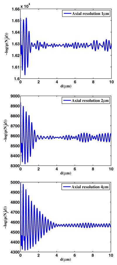
We consider spectra that are Gaussian-shaped, with 1, 2, and 4 μm axial resolutions, respectively. The source power is set at 1 mW to be in compliance with the ANSI standard for the eye safety in this spectral region. We first set the integration time to 5 μs. The truth for the tear film thickness l is set at 0.5 μm, and we assume a root mean square height of the corneal surface of 150 nm [7]. Figure 1 plots the negative log of the conditional probability P(N_l|d), which describes the possibility that observed data N_l is generated by a tear film thickness d. Simulations for three different optical axial resolutions are shown.

Fig. 1.

ML estimator for different axial resolutions.

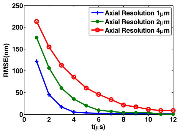
Results show that the probability oscillates with the thickness. The distance between two adjacent peaks is half of the center wavelength in the sample (i.e., 300 nm in the tear film). For a tear film with 0.5 μm thickness, three resolutions of 1, 2, and 4 μm yield estimates of 505, 485, and 545 nm, respectively. It is important to note that estimates beyond the optical axial resolution of this system can be made by this method. However, the precision of the estimation is related to the optical axial resolution, which is further quantified in Fig. 2. Regardless of the integration time, higher optical axial resolution yields higher precision. We also find that among the noise mechanisms we consider, Poisson statistics of the detector is dominant when the system is operated at a longer integration time (i.e., ≫1 μs).

Fig. 2.

Impact of integration time.

In terms of monitoring the tear film dynamics, the imaging speed is a key factor in driving the performance. The two parameters that may affect the imaging speed, the repetition rate of the pulsed source and the integration time of the detector, need to be considered. A first requirement is that the source speed is at least as fast as the detector. Provided that we are not limited by the source speed, we set up a simulation to study the impact of the detector speed, where a tear film thickness of 0.5 μm is considered and we repeat the estimation 5000 times per integration time to quantify how the system performance changes with integration time. The root mean square error (RMSE) is then computed to evaluate the performance for different optical axial resolutions as a function of integration time. Results, plotted in Fig. 2, show that for a fixed axial resolution, the RMSE is decreasing exponentially with an increase in integration time, eventually reaching a stable value in the nanometer range. The trade-offs to consider in pushing the system to a higher speed is the loss in precision. To minimize this loss, a higher axial resolution will be necessary. However, this will cause the possible reduction in imaging depth if the detector array is unchanged. Indeed as the axial resolution increases, the spectral bandwidth increases as well, and for a same size and resolution array, the spectral resolution will consequently be lessened. As such the depth of imaging is also typically reduced.

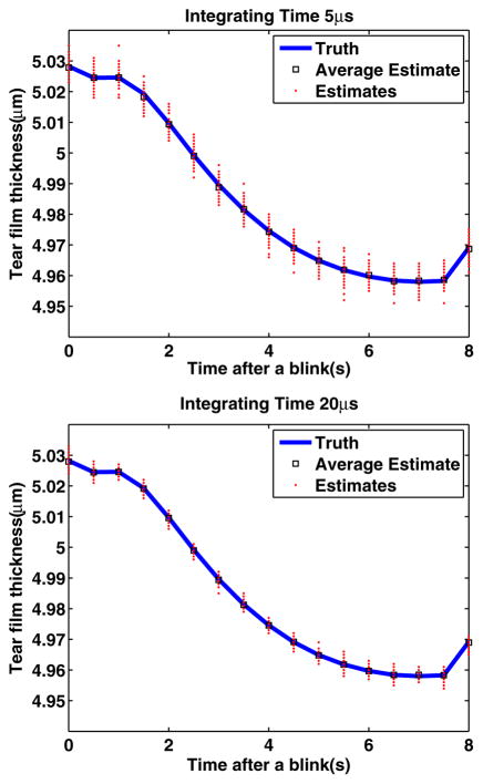
Maki et al. are the first to simulate tear film dynamics on an eye-shaped domain. They studied the relaxation of a model for the human tear film after a blink on a stationary fully opened eye using a mathematical model derived from lubrication theory [8]. The model provides the tear film dynamics data at the center of the cornea, after the eye blinks. While the current model does not yet include evaporation, it still constitutes a useful first digital phantom. We use this model and the ML estimator to estimate the tear film dynamics, operating with an optical axial resolution of 1 μm, and an integration time of 5 and 20 μs, respectively, which is plotted in Fig. 3. Results show that the ML estimates are in agreement with the ground truth, and the ML estimator is unbiased. Results show that as the integration time increases by a factor of 4, the precision is increased by a factor of 2. Results are consistent with findings reported in Fig. 2.

Fig. 3.

Validation with a digital phantom of the tear film dynamics.

In this Letter, we implemented an ML estimator in interpreting OCT data. We quantified the trade-off in temporal resolution against the precision of estimation, which will provide guidance to the operations of the imaging system. For a 20 volumes/s tear film imaging speed (which corresponds to a 5 μs integration time), an axial resolution of less than 2 μm is necessary to keep the precision less than 20 nm; 1 μm axial resolution yields errors in the nanometer scale. Finally, we validated the estimator with a digital phantom of the tear film dynamics. Future studies will, importantly, expand this framework to study other source statistics, theoretically investigate all parameters of the system, and experimentally validate the key parameters established by the model. This framework provides the theoretical tools to develop an optimized OCT system to quantify the tear film dynamics.

References

- 1.Montés-Micó R. J Cataract Refract Surg. 2007;33:1631. doi: 10.1016/j.jcrs.2007.06.019. [DOI] [PubMed] [Google Scholar]
- 2.Sullivan DA, Hammitt KM, Schaumberg DA, Sullivan BD, Begley CG, Gjorstrup P, Garrigue J, Nakamura M, Quentric Y, Barabino S, Dalton M, Novack GD. Ocul Surf. 2012;10:108. doi: 10.1016/j.jtos.2012.02.001. [DOI] [PubMed] [Google Scholar]
- 3.Rolland J, O’Daniel J, Ackay C, De Lemos T, Lee KS, Cheong K-L, Clarkson E, Chakrabarti R, Ferris R. J Opt Soc Am A. 2005;22:1132. doi: 10.1364/josaa.22.001132. [DOI] [PubMed] [Google Scholar]
- 4.Barrett HH, Myers K. Foundations of Image Science. Wiley; 2004. [Google Scholar]
- 5.Huang J, Lee K, Clarkson E, Kupinski M, Maki K, Ross D, Rolland JP. Tech Rep. University of Rochester; 2013. Quantitative measurement of tear film dynamics with optical coherence tomography and statistical decision theory. [Google Scholar]
- 6.Ashtamker Y, Freilikher V, Dainty JC. Opt Express. 2011;19:21658. doi: 10.1364/OE.19.021658. [DOI] [PubMed] [Google Scholar]
- 7.Chen H, Yamabayashi S, Ou B, Tanaka Y, Ohno S, Tsukahara S. Invest Ophthalmol Visual Sci. 1997;38:381. [PubMed] [Google Scholar]
- 8.Maki KL, Braun RJ, Ucciferro P, Henshaw WD, King-Smith PE. J Fluid Mech. 2010;647:361. [Google Scholar]