

Abstract
Infectious disease epidemics such as influenza and Ebola pose a serious threat to global public health. It is crucial to characterize the disease and the evolution of the ongoing epidemic efficiently and accurately. Computational epidemiology can model the disease progress and underlying contact network, but suffers from the lack of real-time and fine-grained surveillance data. Social media, on the other hand, provides timely and detailed disease surveillance, but is insensible to the underlying contact network and disease model. This paper proposes a novel semi-supervised deep learning framework that integrates the strengths of computational epidemiology and social media mining techniques. Specifically, this framework learns the social media users’ health states and intervention actions in real time, which are regularized by the underlying disease model and contact network. Conversely, the learned knowledge from social media can be fed into computational epidemic model to improve the efficiency and accuracy of disease diffusion modeling. We propose an online optimization algorithm to substantialize the above interactive learning process iteratively to achieve a consistent stage of the integration. The extensive experimental results demonstrated that our approach can effectively characterize the spatio-temporal disease diffusion, outperforming competing methods by a substantial margin on multiple metrics.
Keywords: Twitter, deep learning, epidemic simulation
I. Introduction
Infectious disease epidemics such as influenza and Ebola pose a serious threat to global public health. According to a recent World Health Organization (WHO) report [26], seasonal influenza alone is estimated to result in about 3 to 5 million cases of severe illness and about 250,000 to 500,000 deaths each year. In the recent Ebola outbreak in West Africa, there have been 27,055 cases and 11,142 deaths [25]. These diseases share two important characteristics: (1) They spread through close contacts between people; With increased local and global travel, the epidemic is often of large spatial scale. (2) They spread rapidly; for example, during the 2009 H1N1 pandemic, the initial case occurred in Mexico in March 2009; but by the beginning of November 2009, more than 6,000 people had died from H1N1 influenza [23]. In order to take effective public health measures to mitigate such fast-developing epidemics, it is crucial to characterize the disease and the evolution of the ongoing epidemic efficiently and accurately. To handle this problem, recent research in both computational epidemiology and social media mining have achieved important progress and demonstrated their respective usefulness in different aspects.
In the field of computational epidemiology, individual-based network epidemiology has been developed to study the spatio-temporal dynamics of the spread of epidemics. It simulates disease transmission at individual level, and interventions such as vaccinations, school closures, and quarantine. High-performance simulation systems have been developed that are capable of simulating epidemics using network-based models. Such simulations compute the evolution of an epidemic evolution, enabling planners to: (i) forecast the spatio-temporal spread of the disease; (ii) estimate important epidemic measures such as the peak time; and (iii) evaluate the effectiveness of intervention strategies.
Currently, computational epidemiology suffers from the following challenges. 1) Lack of spatially fine-grained surveillance data for model tuning. Existing work mostly relies on surveillance data provided by the Centers for Disease Control and Prevention (CDC) [10] to estimate the model parameters. However, CDC surveillance data only provides state-level spatial information, which is insufficient for accurate diffusion modeling within a state. 2) Difficulties in tracking the dynamics of contact networks in real time. Intervention, such as school closures and vaccinations play an important role in mitigating epidemics by changing people’s infectivity and vulnerability and altering the contact network structure. Current approaches lack effective mechanisms to monitor the impact of ongoing interventions during the current season in real time. 3) High cost and low timeliness of retraining. Existing approaches generally rely on batch training based on the CDC surveillance data. However, CDC surveillance data is updated weekly, with a delay of at least one week, and thus cannot catch up with the real time disease spread.
Social media, on the other hand, can capture timely and ubiquitous disease information from social sensors (i.e., social media users) [11]. Social media-based approaches can be classified into two categories: (i) aggregate-level disease surveillance and (ii) detailed health-informatics analysis. The first category assumes that self-reported symptoms from social media users are reliable signals reflecting the aggregate-level trend of a particular outbreak. Among these, some focus on detecting or tracking current influenza outbreaks while others aim to forecast the severity of the outbreak. The second category focuses on detailed modeling of the social media contents as well as their relevance to health informatics, disease geoinformatics, and health behaviors. However, social media mining approaches suffer from three major drawbacks. First, as a crucial determinant of the disease diffusion pattern, real contact networks are basically unobservable. Estimating social contact networks merely based on the location of social media users is neither accurate nor sufficient. Second, they generally can only characterize the health information of social media users, but not the whole demographic population. Third, they typically only employ the disease information retrieved from social media without utilizing disease model knowledge.
Although computational epidemiology can model the progress of a disease and the underlying disease contact network among individuals, it suffers from a lack of timely and fine-grained surveillance data. Social media mining, on the other hand, provides spatiotemporal surveillance with good timeliness and geographical details, but is unable to observe the underlying contact network and disease progress model. In order to overcome the above-mentioned challenges, we propose a novel online semi-supervised deep learning framework that integrates the strengths of individual-based epidemic simulation and social media mining techniques, named SocIal Media Nested Epidemic SimulaTion (SimNest). SimNest is a novel bispace framework that combines computational epidemiology and social media data by an interactive mapping, as shown in Figure 1. Specifically, on one hand, the health states and interventions actions of social media users are not only identified via their posts by deep learning, but also are regularized unsupervisedly by the disease model in computational epidemiology. On the other hand, the user health states and parametrized disease model learned from social media can provide the computational epidemic model with individual-level surveillance and the optimized disease model parameters. This interactive learning process between social media and computational epidemiolgoy iteratively performs, leading to a consistent stage between these two spaces. The main contributions of our study are summarized as:
Proposing a novel integrated framework for computational epidemiology and social media mining: The existing approaches from computational epidemiology and social media mining focus on different but complementary aspects. The former focuses on modeling the underlying mechanisms of disease diffusion while the latter provides timely and detailed disease surveillance. SimNest framework utilizes both type of information by integrating the strengths of them.
Developing a semi-supervised multilayer perceptron (MLP) for mining epidemic features: To achieve deep integration, we enforce unsupervised pattern constraints derived from epidemic disease progress model onto the supervised classification. Using this semi-supervised strategy, the sparsity of labeled data can be solved.
Designing an online training algorithm: To minimize the inconsistencies between Twitter space and the simulated world, we propose to iteratively optimize model parameters via an online algorithm. This algorithm ingests the social media data streams and updates the model parameters in real time, which not only reduces the cost of retraining but also ensures the timeliness of the model.
Conducting extensive experiments for performance evaluations: The proposed SimNest model was evaluated using Twitter data collected from Jan 2011 to Apr 2015 in 4 states and the District of Columbia in the United States. The proposed methods consistently outperformed competing methods in multiple metrics. The advantage of integrating the complementary strengths of computational epidemiology and social media mining is demonstrated.
Figure 1.
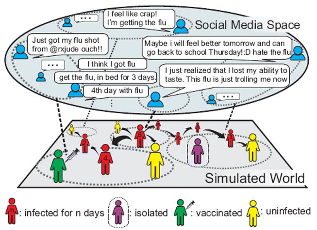
In SimNest, the simulated world mirrors social media space. The posts of social media users reflect their statuses information of health, vaccination, or isolation. This information is mapped to the corresponding spatial subregions in the demographics-based contact network in the simulated world.
II. Related Work
Computational models for epidemiology are important for a number of reasons. Traditionally computational epidemiology focused on compartmental models, where a population is divided into subgroups (compartments) based on people’s health state and demographics, and the epidemic dynamics are modeled by ordinary differential equations [20], [24].
Recently, individual-based computational models have been developed to support network epidemiology, where an epidemic is modeled as a stochastic propagation over an explicit interaction network between people. One common approach taken by network epidemiology is to model the interactions between people using random graph models [13], [16]. Here, the closed form analytical results obtained can be applied to study epidemic dynamics, but this relies on the inherent symmetries in random graphs. With no explicit location modeling, it cannot be applied to compute the geographical spread of an epidemic.
Another direction taken by network epidemiology is to develop a realistic representation of a population by considering members’ social contact network, and then using individual-based simulations to study the spread of epidemics in the network [5], [8]. This approach first constructs a synthetic population, where each individual is assigned demographic, geographic, social, and behavioral attributes so that at various aggregate levels the synthetic population is statistically indistiguishable from the real population. The synthetic individuals are also assigned daily activities and their physical locations at any moment, so by connecting all persons located within close proximity to each other one can construct the corresponding synthetic social contact network for the population [4]. Individual-based simulations model epidemics as diffusion processes across this network, and compute who infects whom at what time at which location [8]. In addition to the synthetic network and disease model, another key component of individual-based epidemic simulations is the associated public health and individual interventions, which can be either pharmaceutical such as vaccination, or non-pharmaceutical such as social distancing. These interventions affect the epidemic evolution by changing the node or edge properties of the network.
Recently, there have been a number of proposals for influenza epidemic knowledge mining techniques based on social media, which can be categorized into two threads. The first thread focuses on aggregate level disease surveillance. For example, Krieck et al. [18] suggested that self-reported symptoms are the most reliable signal in detecting whether a tweet is relevant to an outbreak or not and then went on to demonstrate that this is because even though people generally do not identify their specific problem until diagnosed by an expert, they readily write about how they feel. Using a similar approach to identify flu-related tweets, researchers generally concentrated on tracking the overall trend of a particular disease outbreak, typically influenza, by monitoring social media [2], [14], [17], [28].
The second thread focuses on detailed health-informatics semantic analysis. These approaches typically model the language of the social media messages and their relevance to public health [22] influenza surveillance [12], disease geoinformatics [15], user interactions [9], and health behavior [11]. Paul et al. [22] proposed a topic model that captures the symptoms and possible treatments for ailments, and then went on to propose a way to identify the geographical patterns in the prevalence of such ailments. Specific to self-reporting on influenza, Collier et al. [12] categorized five sub-classes of tweets that serve as user behaviour response surveys for influenza outbreaks, Dredze et al. [15] focused on achieving accurate geographical location identification for influenza outbreak detection, Brennan et al. [9] utilized Twitter user interactions to uncover the health condition of Twitter users. Tackling the problem from a different direction, Chen et al. [11] concentrated on modelling the disease progression in individuals.
III. Problem Setup
This paper aims to characterize the spatiotemporal diffusion of epidemics across the underlying social contact network. Specifically, assume the discrete time increases by interval, and there are T such time intervals T = {0, … , t, … , T}. We aim to know for each time interval t ∈ T the health states Ƶ of the people in the population. Regarding health state transition in a time interval t, we do not distinguish between different moments during the interval when it occurs exactly. To address this problem, approaches based on computational epidemiology and social media mining are formulated in turn below.
A. Individual-based epidemic simulation
A disease transmits through people to people contacts. These people-people contacts form a network called a social contact network G = (V, ε, W), which is a directed, edge-weighted network. Nodes V correspond to individuals in the population. An edge (υ1, υ2) ∈ ε; with weight W(υ1, υ2) denotes the nodes υ1 and υ2 ∈ V has a contact of duration W(υ1, υ2). During the contact the disease may transmit from node υ1 to υ2 with probability p(W(υ1, υ2), τ), where τ, called transmissibility, is probability of transmission per unit of contact time and is a parameter associated with the disease. We first assume that the contact network G is constant. In Section VI, we will consider the situation when G changes with interventions.
Each person is assumed to be in one of the following four health states at any time: susceptible (S), exposed (E), infectious (I), and recovered (R), which is known as the SEIR disease model. It is widely used in the mathematical epidemiology literature [3], [20]. Associated with each person υ are an incubation period pE (υ) and an infectious period pI(υ), each from a distribution. We assume that both are normally distributed, i.e., pE(υ) ~ N(μE, σE) and pI(υ) ~ N(μI, σI). A person is in the susceptible state until he becomes exposed. If a person υ becomes exposed, he remains so for pE(υ) days, during which he is not infectious. Then he becomes infectious and remains so for pI(υ) days. Finally he recovers and remains so. The transition S ↦ E is probabilistic. But we assume that once person υ becomes exposed, pE (υ) and pI(υ) are sampled from the two normal distributions respectively so their values are determined. In sum, given the parameters, let Zυ,t(pE(υ),pI(υ)) ∈ {S,E,I,R} denote the health state of person υ ∈ V on time t ∈ T. Therefore, we have Ƶ = {Zυ,t(pE(υ), pI(υ))}υ∈V,t∈T, where Ƶ stands for peoples’ inferred health states based on individual-based epidemic simulations.
B. Social media based user health state inference
Social media is a popular way for people to post about their everyday feelings, and is commonly treated as a surrogate for the physical world [2]. Taking Twitter as an instance, suppose the set of Twitter users who have ever mentioned their flu infectiousness is denoted as U ⊆ V, which can increase with Twitter data streams. Each user posts nu,t tweets in each time interval t (e.g., hour, day), t = 1, 2, … , T. Define Twitter streams as D = {Du,t}u∈U,t∈T, where the matrix denotes the posts from user u in time t. The (i, j)-th entry, denoted as Du,t,i,j, refers to the frequency of the i-th term in the j-th tweet. V refers to the vocabulary. Suppose we have a predefined subset of keywords K related to flu, and denote A as the corresponding incidence matrix, A ∈ [0,1]|K|×|V|. Define a matrix Xu,t as follows: Xu,t = A · Du,t · 1, where 1 denotes a vector of all ones. It is clear that Xu,t ∈ Z|K| × 1 is the vector of keywords frequencies from user u at time t. Hence, denotes the keyword vectors of user u, while X = {Xu}u∈U denotes the set of all the keyword vectors. We are interested in learning a classifier fW, which maps the social media user textual content Xu,t to their corresponding health states Yu,t:
| (1) |
where Yu,t = 1[Zu,t = I], I stands for “Infectious”, and 1[·] stands for the indicator function. Therefore, Yu,t = 1 signifies that user u’s health state Zu,t at time t is infectious (I); and Yu,t = 0 that it is not. denotes all the health states of user u. W denotes the parameter set of the classifier.
There are three main challenges when using either individual-based epidemic simulation or social media mining techniques individually: (1) There is as yet no surveillance data that is sufficiently real-time and fine-grained to permit the detailed progress of the epidemic simulation to be linked consistently with the physical world. (2) The people-people disease contact network and disease model is hidden to social media data. (3) The fast-streaming and time-evolving nature of huge social media data requires efficient updating of the trained model. Traditional batch-based training suffer from high expense and poor timeliness.
In order to overcome the above-mentioned challenges in either of the above threads individually, we propose using both types of information by deeply integrating the strengths of individual-based epidemic simulation and social media mining techniques in our new framework, SocIal Media Nested Epidemic SimulaTion (SimNest), which is elaborated in the following section.
IV. SimNest Model
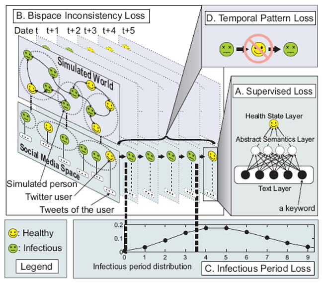
As shown in Figure 2(A), SimNest learns the users’ health states from social media posts based on a multilayer feature representation. Other than considering each time point individually, SimNest utilizes disease progress model in computational epidemiology to constrain the temporal pattern of health states in two aspects: (1) constraining the infectious period to follow a probability distribution in Figure 2(C) and (2) resisting a temporally discontinuous health states like in Figure 2(D). As shown in Figure 2(B), by mapping social media users’ health states into demographics-based synthetic contact network, an interactive learning between these two spaces is achieved. Specifically, simulation model parameters are adjusted by the social media surveillance data while the weights of the multilayer-based health state model are regularized by the underlying synthetic disease contact network.
Figure 2.
The illustration of the SimNest model.
To make the underlying health states in the contact network G consistent with those gathered from social media data D, SimNest simultaneously optimizes contact network, disease progress model parameters pI and pE, and social media-based health state inference fW (·). Among all the keyword vectors X, we are given a set of labeled samples with corresponding class label , and unlabeled samples , where U2 = U − U1 is the set of all the unlabeled users. Mathematically, SimNest model is formulated as jointly minimizing the following four loss functions: (A) Supervised loss, (B) Bispace consistency loss, (C) Infectious duration loss, and (D) Temporal proximity loss, as illustrated as below.
| (2) |
The different loss functions are illustrated in Figure 2. In the following subsections, we will elaborate each of these.
A. Supervised Loss
To effectively build the mapping fw (·) between tweet texts and user health states, which is an abstract concept, we substantialize it by applying deep data representation, namely multilayer perception:
| (3) |
apart from the input layer that is the tweet text and the output layer that is the user health state, another hidden layer represents the abstract semantics, where m is the number of hidden layer features. W = W(1) ∪ W(2), where W(1) ∈ ℝ|K|×m is the weight matrix for the mapping from text layer to abstract semantics layer, W(2) ∈ ℝm×1 is the weight vector for the mapping from abstract semantics layer to the user health status layer and s (·) is the sigmoid function. .
A common way to learn W is to define a loss function over the training data, and then obtain the best W by minimizing the loss of misclassification towards labels:
| (4) |
B. Bispace consistency loss
To sufficiently benefit from the complementary advantages of individual-based epidemic simulation and social media data, the inner inconsistency of the integrated model need to be minimized. Specifically, the hidden health states in the individual-based epidemic simulation need to be consistent with the observations from social media. On the other hand, the intelligence gleaned from the social media data also needs to correspond to the hidden disease progression across the hidden contact network. More formally, our goal is formulated as the following loss function:
| (5) |
where Qυ,t(G, pE, pI) = 1[Zυ,t(pE(υ), pI(υ))= I], and I stands for the state of “infectious”, as introduced in Section III. Θ = {G, pE, pI} are the parameters of individual-based epidemic simulaiton and pE(υ) ~ N (μE, σE) and pI(υ) ~ N (μI, σI) are the incubation and infectious duration distributions of person υ, respectively.
But it is impossible to link the corresponding person to a specific user in Twitter, and not all the people post tweets. Fortunately, however, the specific spatial subregion (e.g., blocks, counties, etc.) of Twitter user u ∈ U and simulated individual υ ∈ V can be known. Hence, the above loss function can be resorted to a fine-grained spatial subregion:
| (6) |
where U2,l denotes the Twitter users in location l, Vl denotes the people in location l, and λ1 is the parameter scaling the person count in the individual-based epidemic simulation down to the count of social media users.
C. Infectious Period Loss
Existing social media mining techniques typically do not assume a specific disease progression model and hence cannot take advantage of its important knowledge pattern. Unlike them, SimNest borrows the disease progression model from the epidemic simulation to regularize the patterns in the huge unlabeled social media data. This not only greatly mitigates the problem of label data sparsity, but also improves the timeliness and generalization of the modeling. Specifically, the infectious duration of a Twitter user is dependent on the flu outbreak’s characteristics as well as his or her general state of physical health, denoted as the following normal distribution:
| (7) |
By maximizing the likelihood function for the observations, we can obtain the following objective function:
which can be transformed to the following formulation by considering Equation 1:
| (8) |
D. Temporal Proximity Loss
Another important intrinsic pattern in the health state modeling is that the states in the neighboring time points should be similar. Moreover, a person recovering from the flu typically cannot get the flu again in the same flu season, as illustrated in Figure 2(D). Thus, the infectious dates are temporally consecutive. This fact motivates the loss function for the proximity of the neighbor states:
| (9) |
V. Online Training Algorithm
To efficiently solve the optimization problem presented in Equation 2, we propose an online parameter optimization framework. It adopts an alternating minimization approach where all variables are fixed except for the one being updated.
A. Solving for W
The process of solving W is based on stochastic gradient descent (SGD) [7]. Training with SGD makes it possible to handle very large databases since every update involves one (or a pair) of examples, and grows linearly in time with the size of the dataset. The convergence of the algorithm is also ensured for low enough values of threshold error.
The derivatives of ℒ1, ℒ3, ℒ3, and ℒ4 can be deduced using backpropagation algorithms and its variants1.
B. Solving for Θ
Solving for Θ = {G,pE,pI} with respect to the loss function ℒ2 is a nonconvex and non-differentiable problem, so a numerical optimization algorithm such as the Nelder- Mead method [7] can be adopted to solve it.
C. Solving for pI, λ1
The sufficient statistics μI and σI of the infectious period distribution pI have the following analytical solution:
| (10) |
| (11) |
Solving for λ1 according to the loss function ℒ2 in Equation 6 yields the following analytical solution:
| (12) |
Utilizing the above alternating optimization process, SimNest is trained and utilized to forecast the spatiotemporal epidemic diffusion progress in the online fashion illustrated in Algorithm 1. Specifically, the unlabeled data set X is continually updated by the social media data streams, with the most out-dated data (such as three months old) being replaced by the newly-arriving data. Then, the weight matrix W is optimized via a SGD fashion until convergence. Utilizing the optimized infectious period distribution as the input for the simulation process, the epidemic simulation parameter pE is optimized by minimizing the inconsistencies with social media data. Finally, the population’s health status Ƶ is predicted. The optimized parameter pE is then utilized for the next-step’s optimization of weight matrix W with the updated unlabeled data. Therefore, as the data is streaming, the parameters is being optimized with the newest data and the predicted health states Ƶ streams out.
|
| |
| Algorithm 1: Online Algorithm for SimNest | |
|
| |
| Input: Data matrix X = X1 ∪ X2, Twitter data stream C, contact network G. | |
| Output: the population’s predicted health states Ƶ. | |
| 1 | Set the learning rate η = 0.5. Initialize weight matrix W as matrix of random values between -1 and 1; |
| 2 | repeat |
| 3 | Update unlabeled data set X2 by Twitter data stream; |
| 4 | repeat |
| 5 | Randomly select a labeled sample (Xu,t, Yu,t); |
| 6 | ; |
| 7 | Randomly select an unlabeled sample Xu; |
| 8 | ; |
| 9 | Randomly select an unlabeled sample Xυ; |
| 10 | for i ← 1 to T do |
| 11 | |
| 12 | end |
| 13 | Randomly select a user u from a location l ∈ L; |
| 14 | ; |
| 15 | ; |
| 16 | ; |
| 17 | until converge; |
| 18 | ; |
| 19 | |
| 20 | until the end of data stream; |
|
| |
VI. Extensions
A. Dynamics of contact network
In the epidemic diffusion progression, interventions are among the most common and effective ways for the government and individuals to reduce the potential impact from disease outbreaks. Interventions influence the epidemic diffusion largely by changing the people-people contact network. They can be categorized into two types: (1) Pharmaceutical (PI) versus (2) Non-pharmaceutical (NPI). PI interventions, such as administering antivirals and vaccines, can change the characteristics (e.g., disease transmissibility) of the person nodes in the social contact network, while NPI interventions are those actions that effectively change the contact network structure, including school closures, quarantine and sequestration. Therefore, both types of interventions can result in changes in the social contact network.
The SimNest framework accommodates these heterogeneous dynamics of contact network effectively via two aspects: (1) Timely intervention actions monitoring based on social media data; and (2) Intervention substantialization through the epidemic simulation process. Take vaccination as an example. First, tweets like “I just got flu shot, it still hurts.” that mention their user Ul’s vaccinations from each subregion l ∈ L are identified by the text classifiers. In our experiments, we achieved a 78% identification accuracy based on the cross-validation results. For example, Figure 3 shows the users who got the flu shots as identified by their Twitter postings during Jan 2011 and Jan 2013 in Virginia. It clearly demonstrates both yearly and weekly periodicity and a peak time around November of each year. The relative vaccination ratio in different subregions can then be estimated as rl = |Ul|/λ1|Vl|, where |Vl| is the size of the population in subregion l and λ1 is the population size scaling factor from the physical world to the Twittersphere, as calculated by Equation 12. Next, in the epidemic simulation SimNest substantializes the vaccinations by reducing the transmissibility p(W(υ1,υ2)), (υ1 ∈ Vl or υ2 ∈ Vl) of rl · |Vl| random individuals in region l by a ratio, which can either be set by domain knowledge or literature.
Figure 3.
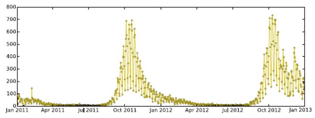
Counts of Twitter users in Virginia who got flu shot
B. Heterogeneous surveillance data
The SimNest framework is also flexible to involve multiple surveillance data sources. In our basic problem definition, we only utilize social media data as a fine-grained surveillance data. Other than that, SimNest allows the addition of heterogeneous surveillance data sources such as CDC [10] surveillance data for the United States, and Paho [21] surveillance data for Latin America. Take CDC surveillance data as an instance, because it is state-level weekly aggregate data, to be comparable to it, SimNest aggregates the predicted user health states into state-level weekly data and involves the following loss function into Equation 2, and get the following equation2:
where C(i) denotes the additional surveillance data on ith time interval. Assume τ′ denotes the time interval between two consecutive data points of C, and τ is the interval of time step of the discrete simulation system. T′ is defined as the number of timepoints of the surveillance data such that T′ = [T · τ′/τ] as= [i · τ′/τ], ae = [(i + 1) τ′/τ] − 1. λ2 is the scaling parameter.
VII. Experiments
In this section, the performance of the proposed SimNest model is evaluated. First, the experiment setup is elaborated. Then, the effectiveness of the SimNest model on state-level influenza epidemic forecasting is demonstrated on real data by comparing with 8 comparison methods. In addition, the performance for forecasting fine-grained geographical subregion is evaluated.
A. Experiment Setup
This subsection presents the data preparation, label set and performance metrics.
1) Dataset
The Twitter data in this paper was retrieved by the following process. First, we query the Twitter API with flu-related keywords and retrieve the data during Jan 1, 2011 and Apr 15, 2015 in the United States. The flu-related keywords include terms such as “flu”, “influenza”, and “h1n1”, among others. The retrieved tweets are then classified according to whether or not they indicate the infection of their authors. The positive tweets are extracted and formed our influenza Twitter set, denoted as D(+). For the classifier, we adopt LibShortText [27], a logistic regression model specially designed for classifying short text like tweets. The classifier is trained on the existing labeled training set provided by Lamb et al. [19]. This training set forms our labeled tweets set, namely the tweets X1 and their labels Y1 in Section IV. The input features K of this model are the disease keywords provided by Paul and Dredze [22].
The authors U2 of the positive tweets set D(+) are extracted and their tweets posted during two weeks before and after their tweets in D(+) are retrieved via Twitter API. After removing retweets, this Twitter data set is geocoded and only those tweets with location of interest are retained to form the unlabeled Twitter data set X2 defined in Section IV. Four states, including Connecticut (CT), Massachusetts (MA), Maryland (MD), and Virginia (VA), and the District of Columbia (DC) are utilized for this performance evaluation. The Carmen geocoder [15] is utilized to resolve the location of each tweet into a tuple containing information at the country, state, county, and city level. About 70% of the tweets in our dataset are assigned with a location by Carmen. To generate the contact network, we utilize the real demographics for each region. Substantial information about Twitter data and the demographics for the five regions are shown in Table I.
Table I.
Twitter data set and demographics
| Demographics | ||||
|---|---|---|---|---|
|
| ||||
| state | population size | #connection | #tweets | #users |
|
| ||||
| CT | 3,518,288 | 175,866,264 | 9,513,741 | 10,257 |
| DC | 599,657 | 19,984,180 | 12,148,925 | 7,015 |
| MA | 6,593,587 | 332,194,314 | 19,785,147 | 15,005 |
| MD | 5,699,478 | 285,159,648 | 20,754,218 | 19,758 |
| VA | 7,882,590 | 407,976,012 | 15,899,713 | 14,302 |
2) Labels and Metrics
For the proposed model and all the competing methods, the data between Aug 1, 2011 and Jul 31, 2012 is utilized as the training season, while the data between Aug 1 2012 and Jul 31 2014 is used for predicting. The forecasting results for the flu outbreaks are validated against the corresponding influenza statistics reported by the Centers for Disease Control and Prevention (CDC). The CDC weekly publishes the percentage of the number of physician visits related to influenza-like illness (ILI) within each major region in the United States. In the experiment, four metrics are adopted, namely mean squared error (MSE), Pearson correlation, p-value, and peak time error. MSE stands for the mean value of the squared errors between all the predicted data points and corresponding label points. Pearson correlation is the covariance of the predicted and label data points divided by the product of their standard deviations. It varies from -1 to 1 and the larger the value, the stronger the positive correlation between them. The p-value denotes how likely the hypothesis of no correlation between the predicted and label data points is true. Thus, the smaller the p-value, the Pearson correlation is more statistically significant. Lastly, peak time error is the time interval between the predicted peak time (i.e., the week with the highest infectious number) and the actual peak time reflected by the CDC label data.
B. State-level influenza epidemic forecasting performance
The performance for forecasting the percentage of ILI visits for each state with different lead times is evaluated. Specifically, the lead time vary from 1 week to 20 weeks, which means every method forecasts the data point from 1 week until 20 weeks in the future. Due to space limitations, we only show the results for Virginia and Connecticut; the results for the other states exhibits the similar patterns to these two. In the experiment, our SimNest model involves the extensions elaborated in Section VI.
1) Comparison methods
Our SimNest model is compared with 6 other methods. Among them, 4 methods are from social media mining: Linear Autoregressive Exogenous model (LinARX) [1], Logistic Autoregressive Exogenous model (LogARX) [2], Simple Linear Regression model (simpleLinReg) [17], Multi-variable linear regression model (multiLinReg) [14]. Another 2 methods are from computational epidemiology: SEIR [20] and EpiFast [6]. Their detailed settings are elaborated in our supplementary materials.
2) Performance on the Pearson correlation and p-value
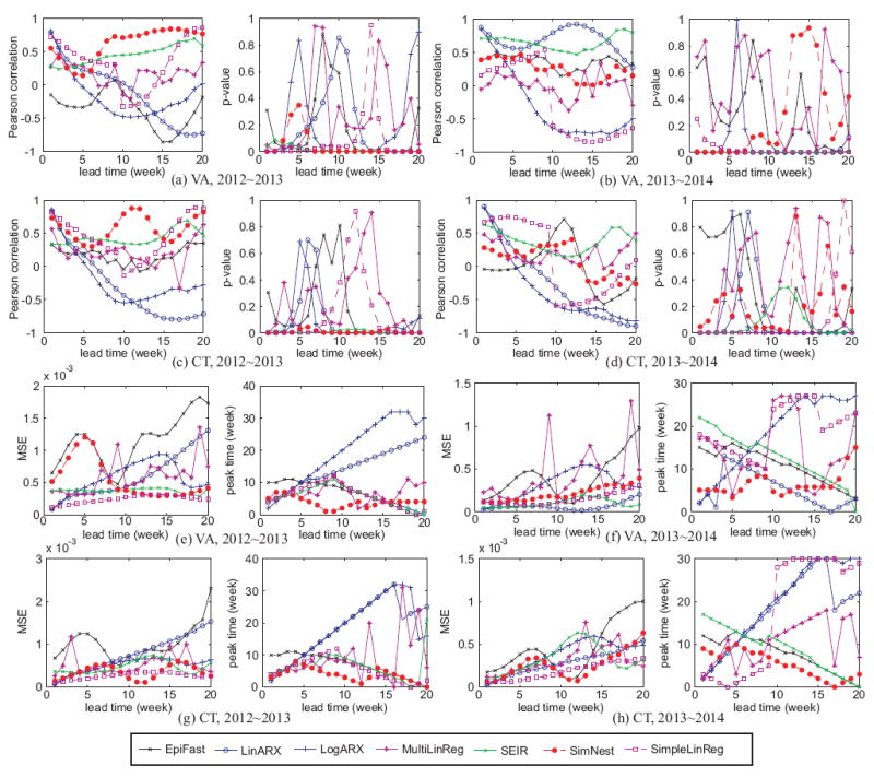
Figure 4(a), 4(b), 4(c), and 4(d) show the forecasting performance in terms of the Pearson correlation and p-value in two states, VA and CT, and for three seasons, 2011-2012, 2012-2013, and 2013-2014. Note that every season starts from August 1st and ends at July 31 each year. Also remember that the training period is 2011-2012 while the rest two seasons are both for testing. Overall, social media-based methods (i.e., LinARX, LogARX, MultiLinReg, and SimpleLinReg) typically achieves high Pearson correlation (i.e., between 0.6-0.95) with small lead time less than 2 weeks, but the Pearson correlation decreases all the way below 0 while lead time increases to 20. The p-value confirms the statistically significance of the high Pearson correlation when the lead time is less than 2 weeks. Computational epidemiology-based methods (i.e., SEIR and EpiFast), on the other hand, performs not as well as social media-based methods with small lead time, but the Pearson correlation does not drop significantly when lead time increases. For example, SEIR still can achieve a Pearson correlation around 0.6 while the lead time is 20 weeks. The reasons are two-folded. First, social media-based methods benefit from the real-time surveillance data while computational epidemiology-based methods use CDC data with a 1-2 week time lag. This difference makes the former one advantageous in predicting data points in the nearest future. Second, social media-based methods are purely data-driven, while computational epidemiology methods make use of the long-term disease progression mechanism. This makes computational epidemiology not too sensitive to current data and more robust in the performance. Among all the methods, our SimNest model performs the best in overall performance by achieving the highest Pearson correlations in Figure 4(a), 4(c), and among the top 3 in Figure 4(b), and 4(d). In addition, the consistent low p-value indicates the robustness of our SimNest model. This result demonstrates that SimNest successfully takes the advantages of the strengths of both social media-based methods and computational epidemiology-based methods.
Figure 4.
ILI visits percentage forecasting performance on the Pearson correlation and p-value for VA and CT in 3 seasons
3) Performance on MSE and peak time error
Figure 4(e), 4(f), 4(g), and 4(h) illustrate the performance on MSE and peak time error of all the methods in VA and CT for three seasons. Similar to the facts reflected by the Pearson correlation in Figure 4, the social media-based methods outperform computational epidemiology-based methods like SEIR and EpiFast in small lead time by achieving low MSE and peak time error. However, while the lead time increases, both the two errors of increase by 5-10 times. Computational epidemiology-based methods consistently achieves a reasonably well MSE and peak time error as low as 2-5 weeks. Our SimNest, again outperforms all the other methods in overall performance. Specifically, It achieves an MSE less than 5 × 10⁻⁴ consistently in both training and testing periods, and achieves the peak time error around 0-4 weeks, which is generally 5-15 weeks less than that of social media-based methods, and at least 3-5 weeks less than that of computational epidemiology-based methods.
C. Spatial subregion outbreaks forecasting performance
Individual-based network epidemiology methods such as EpiFast can model the geographically detailed epidemic outbreaks. To demonstrate the advantage of embedding social media as an individual-level surveillance data, Figure 5 illustrates the comparison between the forecasting of ILI visit percentage for different subregions (i.e., counties) within the Connecticut state. According to Figure 5(a) and 5(b), our SimNest model outperforms EpiFast in the Pearson correlation for Season 2011-2012, Season 2013-2014, and half of Season 2012-2013. The p-values of both methods are less than 0.01 for all the three seasons, showing a statistically significance on the Pearson correlation comparison of them. Finally, our SimNest model again outperforms EpiFast in MSE for Season 2011-2012, Season 2013-2014, and half of Season 2012-2013.
Figure 5.
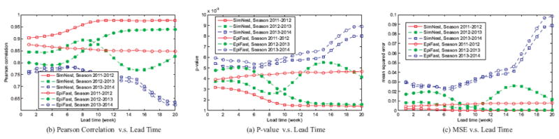
ILI visit percentage forecasting performance for Spatial subregions in CT for three flu seasons
VIII. Conclusions
To achieve timely and accurate epidemic diffusion modeling, computational epidemiology and social media mining communities recently have achieved important progress but still suffer from their different drawbacks. This paper proposes SimNest, a novel bispace co-evolving framework to integrate the complementary strengths of computational epidemiology and social media mining. Extensive experiments based on multiple states and flu seasons demonstrated the advantages of integrating the respective strengths of computational epidemiology and social media mining. The detailed geographical subregion outbreaks forecasting is also improved by using social media that provides individual-level surveillance data.
Acknowledgments
Supported by the Intelligence Advanced Research Projects Activity (IARPA) via DoI/NBC contract number D12PC000337, the US Government is authorized to reproduce and distribute reprints of this work for Governmental purposes notwithstanding any copyright annotation thereon. Disclaimer: The views and conclusions contained herein are those of the authors and should not be interpreted as necessarily representing the official policies or endorsements, either expressed or implied, of IARPA, DoI/NBC, or the US Government. Additionally, this work has been partially supported by DTRA CNIMS Contract HDTRA1- 11-D-0016-0001.
Footnotes
For the detailed deductions, see our supplementary material here: http://people.cs.vt.edu/liangz8/materials/papers/SimNestAddon.pdf
The solution of this equation is in our supplementary material
Contributor Information
Liang Zhao, Email: liangz8@vt.edu, Virginia Tech.
Jiangzhuo Chen, Email: chenj@vbi.vt.edu, Virginia Tech.
Feng Chen, Email: fchen5@albany.edu, University of Albany, SUNY.
Wei Wang, Email: tskatom@vt.edu, Virginia Tech.
Chang-Tien Lu, Email: ctlu@vt.edu, Virginia Tech.
Naren Ramakrishnan, Email: naren@cs.vt.edu, Virginia Tech.
References
- 1.Achrekar H, Gandhe A, Lazarus R, Yu S-H, Liu B. Predicting flu trends using Twitter data. INFOCOM WKSHPS. 2011:702–707. [Google Scholar]
- 2.Achrekar H, Gandhe A, Lazarus R, Yu S-H, Liu B. Biomedical Engineering Systems and Technologies. Springer; 2013. Online social networks flu trend tracker: a novel sensory approach to predict flu trends; pp. 353–368. [Google Scholar]
- 3.Anderson RM, May RM. Population biology of infectious diseases: Part i. Nature. 1979;(280):361–7. doi: 10.1038/280361a0. [DOI] [PubMed] [Google Scholar]
- 4.Barrett C, Beckman R, Khan M, Kumar V, Marathe M, Stretz P, Dutta T, Lewis B. Generation and analysis of large synthetic social contact networks. WSC. 2009 Dec;:1003–1014. [Google Scholar]
- 5.Barrett C, Bisset K, Eubank S, Feng X, Marathe M. Episimdemics: An efficient algorithm for simulating the spread of infectious disease over large realistic social networks. ICS. 2008 Nov;:1–12. [Google Scholar]
- 6.Beckman R, Bisset KR, Chen J, Lewis B, Marathe M, Stretz P. KDD. ACM; 2014. Isis: A networked-epidemiology based pervasive web app for infectious disease pandemic planning and response; pp. 1847–1856. [Google Scholar]
- 7.Bishop CM, et al. Pattern recognition and machine learning. Vol. 4. springer; New York: 2006. [Google Scholar]
- 8.Bisset K, Chen J, Feng X, Kumar VSA, Marathe M. Epifast: A fast algorithm for large scale realistic epidemic simulations on distributed memory systems. ICS. 2009:430–439. [Google Scholar]
- 9.Brennan S, Sadilek A, Kautz H. IJCAI. AAAI Press; 2013. Towards understanding global spread of disease from everyday interpersonal interactions; pp. 2783–2789. [Google Scholar]
- 10.CDC. [May 31, 2015];Fluview interactive. http://www.cdc.gov/flu/weekly/fluviewinteractive.htm.
- 11.Chen L, Hossain KT, Butler P, Ramakrishnan N, Prakash BA. ICDM. IEEE; 2014. Flu gone viral: Syndromic surveillance of flu on Twitter using temporal topic models; pp. 2783–2789. [Google Scholar]
- 12.Collier N, Son NT, Nguyen NM. Omg u got flu? analysis of shared health messages for bio-surveillance. J Biomedical Semantics. 2011;2(S-5):S9. doi: 10.1186/2041-1480-2-S5-S9. [DOI] [PMC free article] [PubMed] [Google Scholar]
- 13.Craft ME, Volz E, Packer C, Meyers LA. Disease transmission in territorial populations: the small-world network of serengeti lions. Journal of the Royal Society Interface. 2011;8(59):776–786. doi: 10.1098/rsif.2010.0511. [DOI] [PMC free article] [PubMed] [Google Scholar]
- 14.Culotta A. Towards detecting influenza epidemics by analyzing Twitter messages; Proceedings of the first workshop on social media analytics; ACM; 2010. pp. 115–122. [Google Scholar]
- 15.Dredze M, Paul MJ, Bergsma S, Tran H. Carmen: A Twitter geolocation system with applications to public health; AAAI Workshop on Expanding the Boundaries of HIAI; Citeseer; 2013. pp. 20–24. [Google Scholar]
- 16.Groendyke C, Welch D, Hunter DR. A network-based analysis of the 1861 hagelloch measles data. Biometrics. 2012;68(3):755–765. doi: 10.1111/j.1541-0420.2012.01748.x. [DOI] [PMC free article] [PubMed] [Google Scholar]
- 17.Hirose H, Wang L. PAAP. IEEE; 2012. Prediction of infectious disease spread using Twitter: A case of influenza; pp. 100–105. [Google Scholar]
- 18.Krieck M, Dreesman J, Otrusina L, Denecke K. A new age of public health: Identifying disease outbreaks by analyzing tweets. WebSci. 2011 [Google Scholar]
- 19.Lamb A, Paul MJ, Dredze M. Separating fact from fear: Tracking flu infections on Twitter. HLT-NAACL. 2013:789–795. [Google Scholar]
- 20.Murray JD. Mathematical biology i: An introduction of interdisciplinary applied mathematics. 2002;17 [Google Scholar]
- 21.PAHO. [May 31, 2015];Paho interactive. www.paho.org/hq/
- 22.Paul MJ, Dredze M. A model for mining public health topics from Twitter. Health. 2012;11:16–6. [Google Scholar]
- 23.Presanis AM, De Angelis D, Hagy A, Reed C, Riley S, Cooper S, Finelli L, Biedrzycki P, Lipsitch M, et al. The severity of pandemic H1N1 influenza in the united states, from april to july 2009: a bayesian analysis. PLoS medicine. 2009;6(12):e1000207. doi: 10.1371/journal.pmed.1000207. [DOI] [PMC free article] [PubMed] [Google Scholar]
- 24.Vynnycky E, White RG. An Introduction to Infectious Disease Modelling. Oxford University Press; 2010. [Google Scholar]
- 25.WHO. [May 29, 2015];Ebola data and statistics. http://apps.who.int/gho/data/view.ebola-sitrep.ebola-summary-latest.
- 26.WHO. [May 15, 2015];Influenza (season) fact sheet. http://www.who.int/mediacentre/factsheets/fs211/en/
- 27.Yu H, Ho C, Juan Y, Lin C. Libshorttext: A library for short-text classification and analysis. Technical report, Technical Report. 2013 http://www.csie.ntu.edu.tw/~cjlin/papers/libshorttext.pdf.
- 28.Zhao L, Chen F, Lu C-T, Ramakrishnan N. SDM. Vol. 15. SIAM; 2015. Spatiotemporal event forecasting in social media; pp. 963–971. [Google Scholar]