A method for avoiding overlap of left and right lungs in shape model guided segmentation of lungs in CT volumes

Abstract

Purpose:

The automated correct segmentation of left and right lungs is a nontrivial problem, because the tissue layer between both lungs can be quite thin. In the case of lung segmentation with left and right lung models, overlapping segmentations can occur. In this paper, the authors address this issue and propose a solution for a model-based lung segmentation method.

Methods:

The thin tissue layer between left and right lungs is detected by means of a classification approach and utilized to selectively modify the cost function of the lung segmentation method. The approach was evaluated on a diverse set of 212 CT scans of normal and diseased lungs. Performance was assessed by utilizing an independent reference standard and by means of comparison to the standard segmentation method without overlap avoidance.

Results:

For cases where the standard approach produced overlapping segmentations, the proposed method significantly (p = 1.65 × 10⁻⁹) reduced the overlap by 97.13% on average (median: 99.96%). In addition, segmentation accuracy assessed with the Dice coefficient showed a statistically significant improvement (p = 7.5 × 10⁻⁵) and was 0.9845 ± 0.0111. For cases where the standard approach did not produce an overlap, performance of the proposed method was not found to be significantly different.

Conclusions:

The proposed method improves the quality of the lung segmentations, which is important for subsequent quantitative analysis steps.

1. INTRODUCTION

Lung segmentation methods are a prerequisite for automated lung image analysis and facilitate tasks like lung volume calculation, quantification of lung diseases, or nodule detection. Many lung segmentation approaches have been proposed that rely on a large density difference between air-filled lung tissue and surrounding tissues.^1–5 Typically, these methods employ gray-level thresholding or region-growing based methods to segment the lung parenchyma and work well for normal lungs. Diseased lungs can have higher density regions (e.g., lung nodules or tumor) and, thus, can pose a problem for region-growing or thresholding-based segmentation methods. To address this issue, we have introduced a robust active shape model-based lung segmentation approach that avoids such shortcomings.⁶ In addition, the method segments left and right lungs independently and, thus, can deal with differently sized left and right lungs, which can occur due to anatomical variation or pathology.

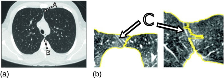
In general, the automated correct segmentation of left and right lungs is a nontrivial problem, because the anterior and posterior junctions between the left and right lungs can be quite thin with low contrast due to partial volume effects (Fig. 1). Consequently, gray-value based lung segmentation approaches (e.g., region growing) can fail to separate the left and right lungs in such areas. Furthermore, techniques that utilize morphological operations to smooth lung boundaries may cause the two lung regions to become connected. Several methods have been devised to separate/split the left and right lungs in the context of gray-value based lung segmentation. Typically, such methods first identify slices that contain a single, large, connected lung component and apply separation methods that detect the thin tissue layer between lungs in regions of interest (ROIs) where a connection between the lungs is suspected.^1,3–5,7 In general, methods that rely on processing of 2D slices have the drawback of potential segmentation inconsistency between slices [Fig. 1(b)].

FIG. 1.

Junction lines between left and right lungs in axial CT images. (a) Image showing a thin tissue layer separating the left and right lung in anterior (A) and posterior (B) junction lines. (b) Example of a 2D lung separation approach that operates on 2D slices and results in segmentation inconsistencies at the anterior junction (C), as depicted in axial (left) and coronal (right) CT image cross-sections.

Leader et al.⁵ and Armato et al.⁴ determine the narrowest region in the anterior–posterior direction and then locate brighter pixels to find the junction lines. Korfiatis et al.³ employ a 2D wavelet preprocessing step to enhance the edges between antero-posterior junction lines. To find the boundary between left and right lungs, many approaches utilize dynamic programming. For example, Hu et al.¹ apply dynamic programming to find a path through a graph with weights proportional to pixel gray-values. The resulting path is assumed to correspond to the boundary between lungs. While they use morphological operations to find the ROI, Rikxoort et al.⁷ simply predefined it based on the center of gravity of the lung region. Park et al.⁸ specified the ROI based on a pair of consecutive CT images and “guide” the dynamic programming algorithm by selecting the start and end points of the search in an adaptive manner. Recently, Lee et al.⁹ proposed a 3D approach based on iterative morphological operations and an Euclidean distance transform to determine a separating surface. If a predefined maximum number of 3D morphological erosion operations is not successful in splitting left and right lungs, the approach utilizes a fallback method where information from a Hessian matrix analysis is incorporated into the erosion process. Consequently, gray-value evidence for the boundary between left and right lungs is only utilized for some data sets (22.7%), which can result in local segmentation (surface separation) errors.

In case of our robust active shape model-based lung segmentation approach⁶ (Fig. 2), the thin tissue layer between lungs can lead to an overlap of left and right segmentation results [Fig. 3(c)], causing local segmentation inaccuracies and a labeling conflict. To address this issue, we propose a classification approach to detect the thin 3D tissue layer between lungs and incorporate this information into the cost function utilized by the robust active shape model (RASM) and subsequent graph-based optimal surface finding (OSF) segmentation method. The performance of our method is demonstrated on 212 lung CT scans. In addition, we provide a comparison of the performance of our proposed approach to the standard segmentation method without overlap avoidance.⁶

FIG. 2.

Schematic diagram showing the RASM–OSF based segmentation pipeline. Note that the segmentation of left and right lungs is done independently.

FIG. 3.

Example of a lung segmentation with and without the sheetness filter approach and corresponding intermediate results. (a) Original CT slice. (b) Standard cost function (Ref. 6), and (c) resulting lung segmentations that are overlapping. (d) Result of the classification-based detection of thin tissue layer between lungs (objects are shown in black). (e) Improved cost function after incorporating the classification result shown in (d). (f) Resulting lung segmentations without overlap.

2. PRIOR WORK

In this section, we give an overview of our previous work on a model-based segmentation method (Fig. 2) that was shown to work well on scans with large (high density) lung cancer masses, which are difficult to segment with region growing approaches.⁶ To generate a lung model that captures the variation in lung shapes, a point distribution model (PDM) is built from total lung capacity (TLC) and functional residual capacity (FRC) lung volumes training data sets. To effectively deal with vastly differently sized left and right lungs, the PDM is built separately for left and right lungs, and all subsequent segmentation steps are done separately as well.

The segmentation procedure begins with initializing the PDM based on a ribs detection step, followed by robustly matching the active shape model to the image volume (RASM segmentation). Subsequently, this segmentation is further refined using a graph-based OSF approach, which allows finding a smooth surface related to the shape prior. In this context, note that both segmentation stages use the same cost function for updating the RASM and OSF-based optimization, respectively (Fig. 2).

The standard cost function previously utilized by us is based on the image gradient computed at a certain scale (i.e., Gaussian smoothed image volume).⁶ This approach prevents attracting the lung surface of the RASM or OSF to features inside the lung (e.g., vessels). However, the smoothing blurs the lung boundary in the thin regions between left and right lungs. This results in low gradient information (high costs) around the posterior and/or anterior junction lines [Fig. 3(b)], which can lead to an overlap of left and right lung segmentations. In this paper, we propose and evaluate a solution for this problem.

3. IMAGE DATA

For this work, 362 multidetector computed tomography (MDCT) thorax scans of lungs were available. The image data consist of three subsets: 196 scans with no significant abnormalities (normals), 78 scans of asthma (42 severe and 36 nonsevere) patients, and 88 scans of lungs with chronic obstructive pulmonary disease (COPD: 24 GOLD 1, 24 GOLD 2, 22 GOLD 3, and 18 GOLD 4). All lungs were imaged at two breathing states: TLC and FRC. The total number of TLC and FRC scans were 181 each. The image sizes varied from 512 × 512 × 351 to 512 × 512 × 804 voxels. The slice thickness of images ranged from 0.50 to 0.70 mm (mean 0.53 mm), and the in-plane resolution from 0.49 × 0.49 to 0.91 × 0.91 mm (mean 0.61 × 0.61 mm). Image volumes were acquired with different MDCT scanners, including Philips Mx8000 as well as Siemens Sensation 64, Sensation 16, and SOMATOM definition flash scanners. The following image reconstruction kernels were utilized: B35, B31, B30, and B.

These data were split into two disjoint sets: one for classifier training and model building and one for evaluation. The PDM (Sec. 2) was built using 150 (75 TLC and 75 FRC) randomly chosen normal lung scans. Out of these, 50 volumes were randomly selected for classifier training (Sec. 4.A.2) to maximize the number of test cases. The rest of the 212 scans were used for evaluation (Sec. 5), resulting in test sets S_normal, S_asthma and S_COPD with 46, 78, and 88 data sets, respectively.

4. METHODS

Our approach to avoiding overlap between left and right lung segmentations is as follows. First, the thin tissue layers between left and right lungs (anterior and posterior junctions) are identified (Sec. 4.A). Second, information about the location of these structures is then utilized to enhance the standard cost function⁶ to form a new improved cost function for RASM and OSF lung segmentations (Sec. 4.B), which avoids overlapping of left and right lung segmentations.

4.A. Identification of thin tissue layers between lungs

The thin tissue layers between left and right lungs are identified by the following two step process.

4.A.1. 3D sheetness filter

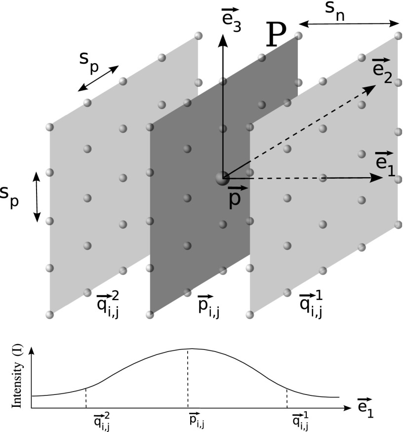
The main purpose of this filter is to detect sheet-like regions (e.g., anterior and/or posterior junction lines) that are of higher density tissue surrounded by lower density tissue (lung). Therefore, two properties are taken into account to obtain a high response at points on the sheet structure in a volume: (i) the intensity at that point must be larger than neighboring points in the direction perpendicular to the sheet and (ii) property (i) should hold consistently for a set of adjacent planar points comprising the sheet. Based on these two criteria, we propose a 3D sheetness filter that is applied to the image volume. Note that because we are looking to detect sheets with small thickness, the sheetness filter is obtained by analyzing the volume at a single scale σ_f. Figure 4 illustrates the filter design, which is described in detail below.

• (a)For a given point $\overrightarrow{p}$, we compute eigenvectors of the Hessian matrix, to find the direction of maximum change at $\overrightarrow{p}$. The eigenvectors are sorted in decreasing order of the absolute value of the corresponding eigenvalues. The first eigenvector $\overrightarrow{e_1}$ represents the direction of the largest change. A plane P is defined based on the second eigenvector $\overrightarrow{e_2}$ and third eigenvector $\overrightarrow{e_3}$ (Fig. 4).
• (b)
  Points are uniformly sampled on this plane P around the point $\overrightarrow{p}$ in k steps along the directions given by $+\overrightarrow{e_2}$, $-\overrightarrow{e_2}$, $+\overrightarrow{e_3}$, and $-\overrightarrow{e_3}$. This gives a sampled point grid of size 2k + 1 × 2k + 1 with a step size of s_p (Fig. 4). The planar points are given by

  $${\displaystyle {\overrightarrow{p}}_{i,j}=\overrightarrow{p}+i{s}_p\overrightarrow{e_2}+j{s}_p\overrightarrow{e_3},}$$ (1)

  with i = − k, …, k and j = − k, …, k.
• (c)
  For each planar point ${\overrightarrow{p}}_{i,j}$, two points in distance s_n are sampled normal to P as follows:

  $${\displaystyle {\overrightarrow{q}}_{i,j}^1={\overrightarrow{p}}_{i,j}+s_n\cdot \overrightarrow{e_1},}$$

  $${\displaystyle {\overrightarrow{q}}_{i,j}^2={\overrightarrow{p}}_{i,j}-s_n\cdot \overrightarrow{e_1}.}$$ (2)
• (d)
  The local gray-value change l_i,j at each planar point ${\overrightarrow{p}}_{i,j}$ is then defined as a function of intensities I at that planar point and corresponding normal point locations and is constrained to be non-negative

  $${\displaystyle l_{i,j}=max(0,I({\overrightarrow{p}}_{i,j})-max(I\left({\overrightarrow{q}}_{i,j}^1\right),I\left({\overrightarrow{q}}_{i,j}^2\right)\left)\right).}$$ (3)

  Equation (3) is related to property (i) mentioned above and results in high values for points on junction lines. Note that the gray-value intensities I were obtained after smoothing the input image with a Gaussian of σ = σ_f.
• (e)
  To fulfill property (ii), local changes l_i,j must be consistently high for all planar points ${\overrightarrow{p}}_{i,j}$ on the plane P. Let $L_{\overrightarrow{p}}=\left\{l_{i,j}\right\}$ with i = − k, …, k and j = − k, …, k denote the set of measured local changes on plane P around location $\overrightarrow{p}$. Then we define a sheetness measure f_sheet as

  $${\displaystyle f_{\mathrm{sheet}}\left(\overrightarrow{p}\right)=\Gamma \left(L_{\overrightarrow{p}}\right),}$$ (4)

  where Γ is a rank order function that computes the average of elements in the first quartile of set $L_{\overrightarrow{p}}$. The choice of function Γ enables suppression of high local responses l_i,j that may arise from other nonplanar high density structures like vessels, while preserving responses from planar structures.

FIG. 4.

Schematic diagram illustrating the design of the sheetness filter and a typical gray-value profile along ${\overrightarrow{e}}_1$ for a point on the sheet-like structure between left and right lungs.

The parameters σ_f and s_n, respectively, determine the minimum and maximum width of sheet like structures that can be found. Parameters k and spacing s_p (distance between sample points) define the extent of the sheet. We qualitatively analyzed ten CT scans and determined that the width of junction lines does not exceed 2 mm. Second, a larger k is preferred to preserve the planar structure but, to avoid the computational overhead, a smaller value of k with a larger value of s_p can be chosen. Based on these observations and qualitative comparison of sheetness response volumes for different combinations of these parameters, the following values have been selected: σ_f = 0.5 mm, s_n = 2 mm, k = 1, and s_p = 3 mm. Typically, the junction between left and right lungs has low curvature, and the selected parameters allow the sheetness filter to detect slightly curved junctions.

4.A.2. Classification of sheetness filter output

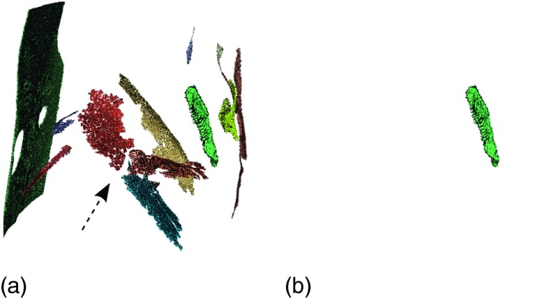
Besides responding to the anterior and posterior junction lines, the sheetness filter also responds to other planar structures like fissures and parts of the CT table, [Figs. 5(b) and 6(a)]. In order to select the structures of interest (anterior and posterior junction lines), a classification approach is utilized.

• (a)Classifier training—For training, the following procedure was performed on a set of 50 training cases described in Sec. 3.
  • (i)
    The sheetness filter response f_sheet [Fig. 5(b)] is computed for all data sets in the training set.
  • (ii)
    A hysteresis thresholding technique with κ₁ (low threshold) and κ₂ (high threshold) is applied to the response f_sheet. A connected component analysis is performed on the two thresholded volumesseparately and components whose size is below δ are removed. The components in the two volumes are combined by the following procedure. Components in the lower threshold volume are kept, if one or more voxels are part of the high threshold image, yielding the component set Φ [Fig. 5(c)].
    In our application, we perform connected component analysis using δ = 100 voxels on two volumes obtained, respectively, using κ₁ = 5 HU and κ₂ = 50 HU.
  • (iii)
    All components ϕ ∈ Φ of the 50 training datasets were manually labeled as structures of interest (using class label η = 1) or background (η = 0), which resulted in 75 and 1530 components, respectively.
  • (iv)
    The structures of interest usually occur at specific locations in the CT volume, have unique shapes [i.e., thin sheets that are more elongated in one direction, as shown in Fig. 6(b)], and show similar orientations. To capture these properties, a 12-dimensional weighted feature vector ${\overrightarrow{f}}_c=\{w_c\overrightarrow{c},w_1\overrightarrow{v_1},w_2\overrightarrow{v_2},w_3\overrightarrow{v_3}\}$ comprising of centroid $\overrightarrow{c}$ and eigenvectors $\overrightarrow{v_i}$ is calculated for each component ϕ ∈ Φ. Note $\overrightarrow{c}$ is the centroid of the component normalized with respect to the size of the image. Eigenvectors $\overrightarrow{v_1}$, $\overrightarrow{v_2}$, and $\overrightarrow{v_3}$ (λ₁ ≥ λ₂ ≥ λ₃) are generated by applying PCA on the coordinates of voxels in ϕ, where λ_i is the eigenvalues associated with $\overrightarrow{v_i}$.
    The weights w_c, w₁, w₂, and w₃ are selected as follows. To capture the elongated shape, the relative length of principal axes is employed: $w_1=\sqrt{{\lambda }_1}/\sum \sqrt{{\lambda }_i}$ and $w_2=\sqrt{{\lambda }_2}/\sum \sqrt{{\lambda }_i}$. To specify the orientation of the sheet, the eigenvector corresponding to the smallest eigenvalue (λ₃) is used and so we set w₃ = 1. Finally, we empirically determined that weighting the centroid $\overrightarrow{c}$ higher than eigenvectors $\overrightarrow{v_i}$ improves the classifier performance. However, too large a weight would reduce performance, because the contribution of $\overrightarrow{v_i}$ would be negligible. Based on a cross-validation experiment on the training data set, we found that an optimal trade-off is achieved with w_c = 6.
  • (v)
    For classification, a support vector machine (SVM) with a radial basis function (RBF) kernel was trained on the features f_c and labels η of all components ϕ ∈ Φ of all 50 training cases. The radius γ of the RBF and regularization parameter C of the classifier are determined by evaluating a discrete set of parameter combinations utilizing five fold cross validation (grid-search approach). Based on the results on training data, a conservative selection was made to decrease the number of false-negatives at the cost of few extra false-positives, resulting in γ = 1 and C = 1. In this context, we observed that the false-positives usually occur outside the body and, thus, do not disturb the segmentation procedure.
• (b)Classifier application—Given a new lung CT volume, the sheetness filter response f_sheet and set Φ of connected components are calculated. Subsequently, the trained SVM classifier is applied to all components ϕ ∈ Φ, and the resulting binary image [Figs. 5(d) and 6(b)] provides the location of thin tissue layer between lungs.

FIG. 5.

Example of identifying the thin tissue layer between lungs. Note that gray-values of figures (b)–(d) are shown inverted for better visibility. (a) Original CT slice. (b) Sheetness response based on the filter described in Sec. 4.A.1. (c) Connected component labeling output after hysteresis thresholding. (d) Binary classification result corresponding to the thin tissue layer between lungs.

FIG. 6.

Filter response caused by fissures and junction lines before and after classification, respectively. (a) Binary image of filter response showing larger sheet-like structures. The left and right lung fissures are clearly visible (arrow). (b) After classification, only the junction line response remains.

4.B. Cost function design

Once the structures of interest are identified [Fig. 5(d)], they are incorporated into the cost function utilized by RASM and OSF segmentation methods. The idea is that the thin tissue layer detected by our classification system provides boundary information in regions between the right and left lungs where the image gradient is weak or nonexistent in the standard cost function image [Fig. 3(b)]. For this purpose, a gradient image $\mathcal{G}$ is created by dilating the binary classified output by 1 voxel [Fig. 3(d)] and applying a gradient operator at a scale of 1 mm. The magnitude of $\mathcal{G}$ is scaled by a constant scalar (1800) so that it is approximately two times the largest magnitude in the standard cost function, in order to make sheet structure between lungs more attractive for the RASM and OSF segmentation methods. The gradient image $\mathcal{G}$ is then added to the standard cost function image to yield a new improved cost function [Fig. 3(e)].

Figures 3(c) and 3(f) provide a comparison between a segmentation result generated with standard and improved cost function design, respectively.

5. EVALUATION

5.A. Independent reference standard

For all tested data sets (Sec. 3), an independent reference standard was generated by first using a commercial lung image analysis software package Apollo (VIDA Diagnostics, Inc., Coralville, IA) to automatically create lung segmentations. These were then inspected by a trained expert under the supervision of pulmonologist and segmentation errors were manually corrected.

5.B. Quantitative indices

For performance assessment, the following quantitative indices are utilized to assess overlap between right and left lungs as well as segmentation accuracy.

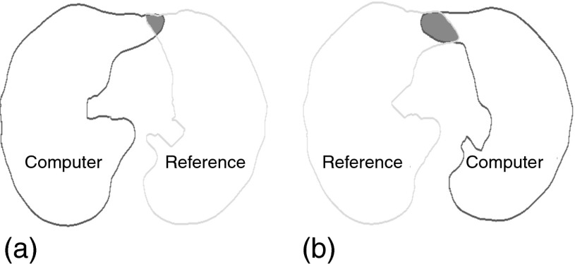
• (i)Overlap between lungs—To quantify the degree of segmentation overlap between right and left lung segmentations, we compute the amount of overlap a given segmentation produces with the adjacent reference lung segmentation. For example, the left lung segmentation is compared with the right lung reference and vice versa, as shown in Fig. 7. The number of overlapping voxels is denoted by Ω and is computed separately for left and right lungs. In addition, the mutual overlap between algorithm generated left and right lung segmentations is assessed with ξ, which denotes the number of voxels that are overlapping. The advantage of using Ω is that it gives a correct indication of how much a lung segmentation has “leaked” into the adjacent lung, which may not be captured using ξ alone (e.g., when both lung segmentations are incorrect and have minimal overlap between them).
• (ii)Segmentation accuracy—To assess the impact of our approach on segmentation accuracy, we utilize the Dice coefficient D (Ref. 10) and evaluate accuracy independently for left and right lungs.

FIG. 7.

Quantification of segmentation overlap between reference and computer generated segmentations. The overlap is shown as shaded region and is assessed for right (a) and left (b) lung segmentations separately.

5.C. Experimental setup

The PDM was built using 150 (75 TLC and 75 FRC) normal lung scans (Sec. 3). Our implementation of model-based lung segmentation is based on the standard approach⁶ but with one difference. Both the RASM model matching and OSF-based refinement are applied to volumes from which major airways are excluded, as follows. The trachea and main bronchi in test volumes are first extracted by utilizing a modified system of the airway tree segmentation method.¹¹ Resulting airway structures are then dilated using a radius of 2 voxels. Subsequently, a value of 50 HU is assigned to locations in the input volume that corresponded to airways. This makes the airways unattractive for RASM and OSF segmentation.

The model-based RASM–OSF algorithm is applied to each image using two methods with different cost functions. Method 1 (M1) uses the standard image gradient based cost function,⁶ and Method 2 (M2) employs the improved cost function described in Sec. 4.B. Since the RASM–OSF algorithm computes an intermediate (RASM) and final (OSF) segmentations, we qualify the notation for quantitative indices accordingly. For example, ${\Omega }_{\mathrm{M1}}^{\mathrm{OSF}}$ represents the degree of overlap obtained by method M1 based on OSF segmentation.

For segmentation accuracy assessment, we divide the experiments into two parts. First, lungs that have initially overlapping final segmentations $({\Omega }_{\mathrm{M1}}^{\mathrm{OSF}}>0)$ are considered. Second, nonoverlapping segmentations $({\Omega }_{\mathrm{M1}}^{\mathrm{OSF}}=0)$ are assessed. Table I provides the total number of left and right lung volumes combined that were available for evaluation in these two categories.

TABLE I.

Number of left and right lung volumes utilized for evaluation that initially show and do not show an overlap.

Set	Number of overlapping cases $({\Omega }_{\mathrm{M1}}^{\mathrm{OSF}}>0)$	Number of nonoverlapping cases $({\Omega }_{\mathrm{M1}}^{\mathrm{OSF}}=0)$
Snormal	38	54
Sasthma	39	117
SCOPD	65	111
TLC	107	105
FRC	35	177
ALL	142	282

6. RESULTS

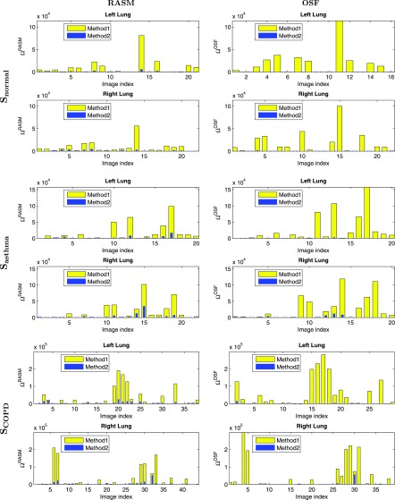
Figure 8 shows the overlap measure Ω for methods M1 and M2 for the three different test data sets. Note that in addition to the final OSF results of the lung segmentation method, the intermediate RASM results were also assessed and summarized in Fig. 8. In addition, cases for which both Ω_M1 = 0 and Ω_M2 = 0 were omitted to increase the readability of the graphs. Overall, the intermediate output ${\Omega }_{\mathrm{M2}}^{\mathrm{RASM}}$ was found to be statistically significant improved compared to ${\Omega }_{\mathrm{M1}}^{\mathrm{RASM}}$ based on a paired t-test (p = 1.92 × 10⁻⁸). The final outputs ${\Omega }_{\mathrm{M1}}^{\mathrm{OSF}}$ and ${\Omega }_{\mathrm{M2}}^{\mathrm{OSF}}$ were compared utilizing a paired t-test, and the results are provided in Table II in combination with other statistics.

FIG. 8.

Degree of overlap assessed with Ω for all three datasets. The bar plot for Method 2 is drawn on top of Method 1. The first column shows results for the intermediate RASM segmentations while the second column shows results for the final OSF segmentations.

TABLE II.

Overlap statistics computed from final lung segmentations. Note that * indicates p-values that were statistically significant.

Set	Statistics	${\Omega }_{\mathrm{M1}}^{\mathrm{OSF}}$	${\Omega }_{\mathrm{M2}}^{\mathrm{OSF}}$	Overlap reduction (%)	p-value of paired t-test
Snormal	First quartile	139	0	100	3.34 × 10−4*
	Median	8 678	0	100
	Third quartile	25 259	11	99.96
	Mean	16 321	44	99.73
Sasthma	First quartile	655	0	100	2.21 × 10−4*
	Median	9 028	4	99.96
	Third quartile	31 379	229	99.27
	Mean	26 214	994	96.21
SCOPD	First quartile	102	0	100	1.58 × 10−5*
	Median	3 083	2	99.94
	Third quartile	48 388	155	99.68
	Mean	45 293	1393	96.93
ALL	First quartile	204	0	100	1.65 × 10−9*
	Median	4 893	2	99.96
	3rd Quartile	32 934	73	99.78
	Mean	32 525	932	97.13

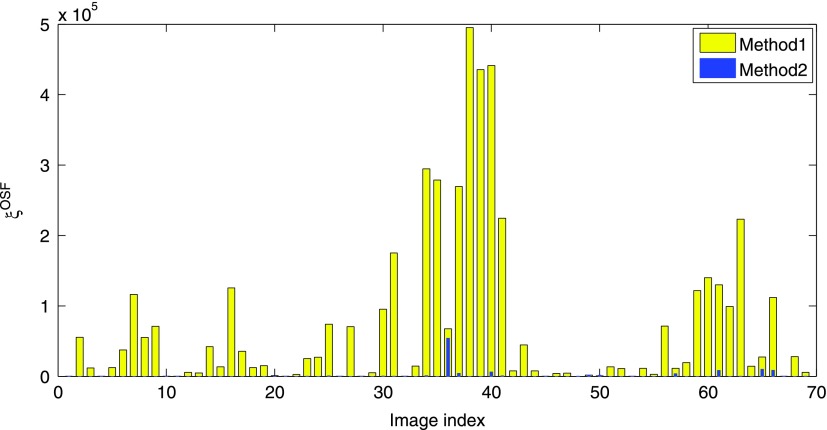
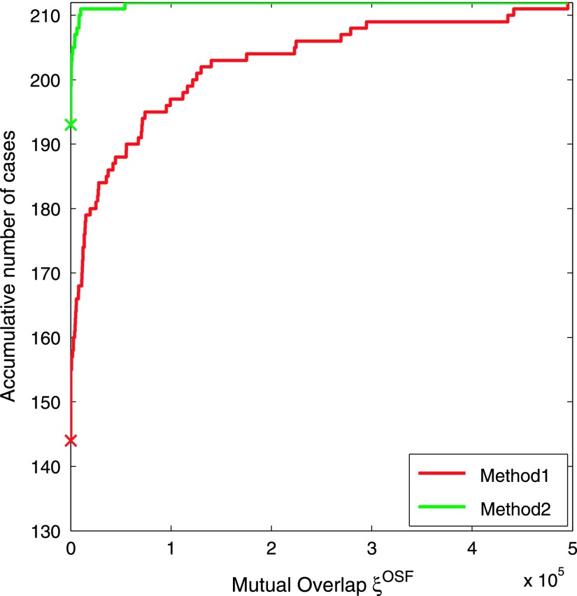
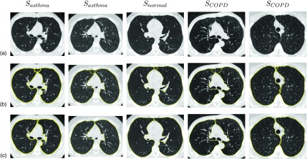
A plot of ξ^OSF, assessing the mutual overlap between left and right segmentations, is provided in Fig. 9. As before, cases where both ${\xi }_{\mathrm{M1}}^{\mathrm{OSF}}=0$ and ${\xi }_{\mathrm{M2}}^{\mathrm{OSF}}=0$ were omitted to increase the readability of the graph. The mean mutual overlap reduces from 68 482 voxels to 1462 voxels (97.87%), and the median from 14 571 to 0 voxels (100%). Based on a paired t-test, the reduction was found to be statistically significant (p = 3.51 × 10⁻⁶). Figure 10 depicts the accumulative number of test cases as a function of mutual overlap ξ^OSF for both methods. Examples of final segmentations for Methods 1 and 2 are given in Fig. 11.

FIG. 9.

Mutual overlap ξ^OSF between left and right lung segmentations for test cases (see text in Sec. 6). The bar plot for Method 2 is drawn on top of Method 1.

FIG. 10.

Accumulative number of test cases as a function of mutual overlap ξ^OSF between left and right lung segmentations for all 212 test data sets. For each method, a cross on the vertical axis indicates the number of overlap-free cases (Method 1: 67.9% and Method 2: 91.0%).

FIG. 11.

Comparison of final segmentations results. (a) Original axial CT images. (b) Results produced by Method 1. (c) Results produced by Method 2.

To assess segmentation accuracy, Table III summarizes the mean and standard deviation of D^OSF for initially overlapping lung segmentations and different volume sets as well as the outcome of a paired t-test. Note that Method 2 shows a statistically significant improvement on all sets and for both TLC and FRC scans. For nonoverlapping lungs, Table IV provides mean and standard deviation values for D^OSF. Note that, for these cases, the differences between methods were not found to be statistically significant. Also, the test data sets have different complexity. Specifically, there are some test cases that are more challenging to segment with a model-based lung segmentation approach than others, which affects both methods roughly equally. Consequently, this leads to somewhat increased standard deviation values in Tables III and IV, but does not affect the paired t-test.

TABLE III.

Dice coefficient D^OSF for initially overlapping cases. Note that * indicates p-values that were statistically significant. Higher average segmentation performance is shown in bold.

Set	$D_{\mathrm{M1}}^{\mathrm{OSF}}$ (×10−2)	$D_{\mathrm{M2}}^{\mathrm{OSF}}$ (×10−2)	p-value of paired t-test
Snormal	98.63 ± 0.92	98.69 ± 0.97	6.54 × 10−3*
Sasthma	98.15 ± 1.71	98.28 ± 1.65	7.92 × 10−5*
SCOPD	98.21 ± 1.10	98.41 ± 0.70	8.36 × 10−3*
TLC	98.42 ± 1.40	98.55 ± 1.22	3.04 × 10−3*
FRC	97.96 ± 0.63	98.15 ± 0.58	2.73 × 10−3*
ALL	98.31 ± 1.26	98.45 ± 1.11	7.50 × 10−5*

TABLE IV.

Dice coefficient D^OSF for initially not overlapping cases. Higher average segmentation performance is shown in bold.

Set	$D_{\mathrm{M1}}^{\mathrm{OSF}}$ (×10−2)	$D_{\mathrm{M2}}^{\mathrm{OSF}}$ (×10−2)	p-value of paired t-test
Snormal	98.27 ± 0.60	98.27 ± 0.59	0.91
Sasthma	97.33 ± 2.26	97.34 ± 2.20	0.58
SCOPD	97.96 ± 1.55	98.00 ± 1.31	0.28
TLC	98.41 ± 1.04	98.40 ± 0.99	0.79
FRC	97.38 ± 2.04	97.41 ± 1.91	0.21
ALL	97.76 ± 1.80	97.78 ± 1.70	0.26

Calculating a sheetness response volume [e.g., Fig. 5(b)] required on average 5.07 ± 0.52 min of computing time on a PC with a 2.70 GHz Intel Xeon(R) CPU. The hysteresis-based connected component labeling and classification took an average of 54 ± 20 s, and the RASM–OSF based segmentation required 6 min. All implementation were done in C++, except for SVM training and classification, which was performed in matlab (The MathWorks, Inc., MA) by utilizing matlab’s Statistics Toolbox (version 8.0).

7. DISCUSSION

The evaluation on a diverse set of 212 CT scans of normals and diseased lungs at two different breathing states has shown that the proposed approach significantly reduces/eliminates overlap between left and right lung segmentations of our model-based segmentation approach. The segmentation accuracy (i.e., Dice coefficient) was found to be increased (Method 2) for cases that showed an overlap when processed with standard cost function (Method 1). The small amount of increase can be explained by the fact that the volume of a lung is large relative to volume error induced by the overlap. Nevertheless, the improvement was statistically significant in all cases. Also, for data sets that did not cause an overlap when processed with Method 1, the average Dice coefficient of Method 2 was in the same range as for Method 1 with no statistical significant difference. This shows that our approach does not deteriorate segmentation accuracy for cases where no overlap between right and left occurred when processed with Method 1.

The comparison of RASM and OSF performance of Method 1 and Method 2 in Fig. 8 shows that typically ${\Omega }_{\mathrm{M1}}^{\mathrm{RASM}}<{\Omega }_{\mathrm{M1}}^{\mathrm{OSF}}$, but ${\Omega }_{\mathrm{M2}}^{\mathrm{RASM}}>{\Omega }_{\mathrm{M2}}^{\mathrm{OSF}}$. This can be explained as follows. The RASM segmentation is more constrained than the OSF segmentation approach, because the RASM is based on a shape model. For the standard approach (Method 1), this means that an overlap assessed with Ω can get worse with OSF segmentation, because only weak or no gradient information is present at junctions between left and right lungs. In contrast, the proposed approach (Method 2) provides gradient information at junctions, which reduces the overlap and improves segmentation performance.

As the statistics in Table II show, the overlap has been significantly reduced. However, in 19 out of 212 test cases, a minimal amount of overlap occurred (Fig. 10). Their examination showed that in the majority of them, the overlap was not caused by the presence of thin junction lines, but occurred due to other factors like variations in lung shapes (e.g., asymmetric lung shapes). Such issues that are related to shape can be addressed by including representative examples in the lung model building process. In one case, a subpart of a junction was not correctly classified, because similar examples were not included in the training data set. A larger (diverse) training set would allow to address this issue. Similarly, our method can be adapted to other imaging protocols (e.g., different location or orientation of junction lines), etc., by training of the classifier.

In the future, we plan on investigating if our approach can be further improved by eliminating remaining inconsistencies resulting in segmentation overlap by utilizing a simultaneous OSF-based mutual segmentation of both lungs, similar as utilized for bone and cartilage segmentation of the human knee joint.¹²

Our thin tissue layer detection (classification) approach works inherently in 3D and, thus, avoids typical inconsistencies of slice-per-slice based detection approaches [Fig. 1(b)] that were utilized in combination with gray-value based lung segmentation methods to split merged left and right lungs.^1,4,5,7 Also, because the employed lung segmentation approach⁶ already utilizes a 3D OSF approach (i.e., search of a closed surface), information about the location of thin tissue layer can be seamlessly integrated without the need to find start and end points, as required for 2D dynamic programming based methods in the context of conventional gray-value based lung segmentation methods,^1,7,8 which is error prone. Another advantage of our approach is that local image features calculated by our approach show responses on fissures [Fig. 6(a)] and, therefore, could potentially be utilized for lung fissure localization, which is frequently a subsequent step to lung segmentation.

Computing the sheetness response requires additional computing time (Sec. 6). However, as outlined above, the utilized sheetness filter typically represents a core-component of a subsequent fissure detection approach. Thus, in most cases, synergies can be realized, resulting in low additional costs for our approach. Alternatively, a simple heuristic can be used to reduce computing time. For example, junction lines typically occur in a small band near the center of the body. Thus, features could only be calculated at those locations.

8. CONCLUSIONS

For a robust model-based segmentation approach, we have presented a method that addresses the problem of overlapping left and right lung segmentations. The method employs a classification approach to detect thin tissue regions between lungs in close proximity and selectively incorporates them into the previously developed cost-function of the utilized RASM–OSF segmentation framework. The proposed method works inherently in 3D. Consequently, inconsistencies between neighboring slices can be avoided. The performed evaluation has demonstrated that the overlap between left and right lungs was significantly reduced. Consequently, the method improves the quality of lung segmentations produced by our model-based segmentation approach. This is especially important for applications requiring an accurate lung mask for automated quantitative assessment of lung diseases.

REFERENCES

- 1.Hu S., Hoffman E. A., and Reinhardt J. M., “Automatic lung segmentation for accurate quantitation of volumetric x-ray CT images,” IEEE Trans. Med. Imag. 20, 490–498 (2001). 10.1109/42.929615 [DOI] [PubMed] [Google Scholar]
- 2.Kuhnigk J.-M., Dicken V., Zidowitz S., Bornemann L., Kuemmerlen B., Krass S., Peitgen H.-O., Yuval S., Jend H.-H., Rau W. S., and Achenbach T., “New tools for computer assistance in thoracic CT. Part 1. Functional analysis of lungs, lung lobes, and bronchopulmonary segments,” Radiographics 25(2), 525–536 (2005). 10.1148/rg.252045070 [DOI] [PubMed] [Google Scholar]
- 3.Korfiatis P., Skiadopoulos S., Sakellaropoulos P., Kalogeropoulou C., and Costaridou L., “Combining 2D wavelet edge highlighting and 3D thresholding for lung segmentation in thin-slice CT,” Br. J. Radiol. 80(960), 996–1004 (2007). 10.1259/bjr/20861881 [DOI] [PubMed] [Google Scholar]
- 4.Armato S. G. and Sensakovic W. F., “Automated lung segmentation for thoracic CT: Impact on computer-aided diagnosis,” Acad. Radiol. 11(9), 1011–1021 (2004). 10.1016/j.acra.2004.06.005 [DOI] [PubMed] [Google Scholar]
- 5.Leader J. K., Zheng B., Rogers R. M., Sciurba F. C., Perez A., Chapman B. E., Patel S., Fuhrman C. R., and Gur D., “Automated lung segmentation in X-ray computed tomography: Development and evaluation of a heuristic threshold-based scheme,” Acad. Radiol. 10(11), 1224–1236 (2003). 10.1016/S1076-6332(03)00380-5 [DOI] [PubMed] [Google Scholar]
- 6.Sun S., Bauer C., and Beichel R., “Automated 3D segmentation of lungs with lung cancer in CT data using a novel robust active shape model approach,” IEEE Trans. Med. Imag. 31(2), 449–460 (2012). 10.1109/TMI.2011.2171357 [DOI] [PMC free article] [PubMed] [Google Scholar]
- 7.van Rikxoort E. M., de Hoop B., Viergever M. A., Prokop M., and van Ginneken B., “Automatic lung segmentation from thoracic computed tomography scans using a hybrid approach with error detection,” Med. Phys. 36(7), 2934–2947 (2009). 10.1118/1.3147146 [DOI] [PubMed] [Google Scholar]
- 8.Park S. C., Leader J. K., Tan J., Lee G. S., Kim S. H., Na I. S., and Zheng B., “Separation of left and right lungs using 3D information of sequential CT images and a guided dynamic programming algorithm,” J. Comput. Assist. Tomogr. 35(2), 280–289 (2011). 10.1097/RCT.0b013e31820e4389 [DOI] [PMC free article] [PubMed] [Google Scholar]
- 9.Lee Y. J., Lee M., Kim N., Seo J. B., and Park J. Y., “Automatic left and right lung separation using free-formed surface fitting on volumetric CT,” J. Digital Imag. 27(4), 538–547 (2014). 10.1007/s10278-014-9680-5 [DOI] [PMC free article] [PubMed] [Google Scholar]
- 10.Sonka M., Hlavac V., and Boyle R., Image Processing, Analysis, and Machine Vision (Thompson Learning, Toronto, 2008). [Google Scholar]
- 11.Bauer C., Pock T., Bischof H., and Beichel R., “Airway tree reconstruction based on tube detection,” in Proceedings of the Second International Workshop on Pulmonary Image (CreateSpace, London, UK, 2009), pp. 203–213. [Google Scholar]
- 12.Yin Y., Zhang X., Williams R., Wu X., Anderson D., and Sonka M., “LOGISMOS—Layered optimal graph image segmentation of multiple objects and surfaces: Cartilage segmentation in the knee joint,” IEEE Trans. Med. Imag. 29(12), 2023–2037 (2010). 10.1109/TMI.2010.2058861 [DOI] [PMC free article] [PubMed] [Google Scholar]