Biostatistics Series Module 4: Comparing Groups – Categorical Variables

Abstract

Categorical variables are commonly represented as counts or frequencies. For analysis, such data are conveniently arranged in contingency tables. Conventionally, such tables are designated as r × c tables, with r denoting number of rows and c denoting number of columns. The Chi-square (χ²) probability distribution is particularly useful in analyzing categorical variables. A number of tests yield test statistics that fit, at least approximately, a χ² distribution and hence are referred to as χ² tests. Examples include Pearson's χ² test (or simply the χ² test), McNemar's χ² test, Mantel–Haenszel χ² test and others. The Pearson's χ² test is the most commonly used test for assessing difference in distribution of a categorical variable between two or more independent groups. If the groups are ordered in some manner, the χ² test for trend should be used. The Fisher's exact probability test is a test of the independence between two dichotomous categorical variables. It provides a better alternative to the χ² statistic to assess the difference between two independent proportions when numbers are small, but cannot be applied to a contingency table larger than a two-dimensional one. The McNemar's χ² test assesses the difference between paired proportions. It is used when the frequencies in a 2 × 2 table represent paired samples or observations. The Cochran's Q test is a generalization of the McNemar's test that compares more than two related proportions. The P value from the χ² test or its counterparts does not indicate the strength of the difference or association between the categorical variables involved. This information can be obtained from the relative risk or the odds ratio statistic which is measures of dichotomous association obtained from 2 × 2 tables.

Introduction

Categorical variables commonly represent counts or frequencies. Count data usually pertains to subjects or articles with certain attributes, exposures or outcomes and is represented by non-negative integers. Thus, in a group, one may count the number of individuals who are tall, or have been exposed to a viral disease or may have survived lung cancer. For analysis, such data are conveniently arranged in a contingency table.

Such a table provides the frequencies for two or more categorical variables simultaneously and can be constructed by cross-classification (cross-tabulation) of the counts on two or more variables. A table that depicts the frequencies of two variables would be called a two-way or two-dimensional contingency table. In the simplest case, as depicted in Table 1, the table will have 2 rows and 2 columns, and therefore would be a 2 × 2 (two-by-two) table. A table with r rows and c columns would be referred to as r × c contingency table.

Table 1.

Example of a two-dimensional or two-way contingency table

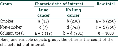
Note that, in such a table, each subject would be counted in only one cell, the one corresponding to that particular combination of variable categories. The summation of the counts in all the cells would give the total number of subjects in the study. In the example presented in Table 1, the grouping variable is placed in rows, which is the usual convention. In epidemiological studies, exposure categories are generally placed in rows and outcome categories in columns. For example when we are examining the relationship between smoking and lung cancer, the exposure categories, namely ‘smokers’ and ‘nonsmokers’, would be placed in rows, while the outcome categories, namely ‘lung cancer’ and ‘no lung cancer’ would be placed in columns.

In contingency tables, once the row and column totals are known, only some of the cells can take independent values. The values in other cells would then be constrained by the row and column totals. Therefore, a contingency table is said to have certain degrees of freedom (df), calculated as (r − 1) × (c − 1). Thus, a 2 × 2 table will have df = 1, whereas a 3 × 3 table will have df = 4. In the example in Figure 1, once we know that there are 250 smokers and 750 nonsmokers in the study, and that there are total 19 individuals with lung cancer, we can ascribe an independent value to only one of the cells. The values in the other cells would then be automatically determined by the row and column totals.

Figure 1.

Common statistical tests to compare categorical data for difference

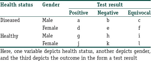
The analysis of such two-dimensional contingency tables often involves testing for the difference between the two groups using the familiar Chi-square (χ²) test and its variants. Three- and higher-dimensional tables are dealt with by multivariate log-linear analysis. In Table 2, we provide an example of a three-way contingency table that depicts frequencies simultaneously for three categorical variables, namely, health status, gender, and test result. In the analysis of such a table, the log-linear model can be used which, however, is outside the scope of this module.

Table 2.

Example of a three-dimensional or three-way contingency table

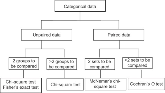
Before we take up individual tests, and their variants used to assess categorical or count-type data, let us recapitulate through Figure 1, the tests that are available to compare groups or sets of categorical data for a significant difference.

Chi-square Distribution

This is a continuous probability distribution given by positive values that are skewed to the right. The shape of a χ² distribution is characterized by its df. As the df increases, it becomes more symmetrical and approaches the normal distribution. Figure 2 depicts a set of χ² distributions with varying df. Thus, like the t-distribution, the χ² distribution represents a whole family of distributions distinguished by the df parameter, but unlike the t-distribution, it is not symmetrical. However, for df values greater than about thirty, it will approximate the normal distribution.

Figure 2.

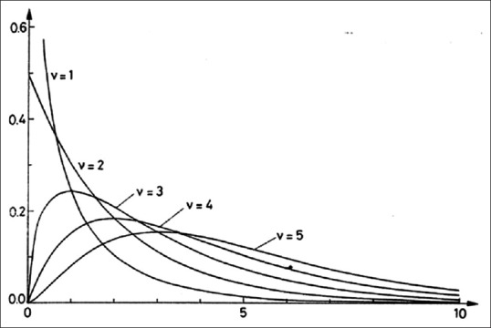
Chi-square distributions with different degrees of freedom. The X-axis denotes the χ² value, whereas the Y-axis denotes the probability density function. Note that as degree of freedom (ν) increases the distribution is tending to become more symmetrical

This distribution is particularly useful in analyzing categorical variables. A number of statistical tests yield test statistics that fit, at least approximately, a χ² distribution and hence they may be referred to as χ² tests. Examples include Pearson's χ² test (also simply called the χ² test), McNemar's χ² test, Cochran–Mantel–Haenszel χ² test, and others.

Chi-square Test

The Pearson's χ² test (after Karl Pearson, 1900) is the most commonly used test for the difference in distribution of categorical variables between two or more independent groups.

Suppose we are interested in comparing the proportion of individuals with or without a particular characteristic between two groups. The null hypothesis would be that there is no difference between these two proportions. The data can be arranged in a 2 × 2 contingency table. We will need a larger contingency table to arrange the data if there are more than two groups or the categorical variable of interest can take more than two possible values.

Depending on the observed frequencies in each cell, the test involves in calculating the corresponding expected frequencies. The expected frequency is calculated by dividing the product of the applicable row and column total for that cell by the overall total. The test then finds out if the observed counts differ significantly from the expected counts, if there was no difference between groups. The Pearson χ² statistic is calculated as:

where O: The observed count in each cell, and E: The expected count in that cell.

The calculated value of the χ² statistic is referred to the χ² distribution table, and the resultant significance level (P value) depends on the applicable df. If the P value is less than the selected critical value (say 0.05 or 0.01) then the null hypothesis can be rejected.

When testing for independence in a contingency table, the χ² distribution, which is a continuous probability distribution, is used as an approximation to the discrete probability of observed frequencies, namely the multinomial distribution. When the total number of observations is small, the estimates of probabilities in each cell become inaccurate and the risk of Type I error increases. It is not fixed how large N should be, but probably at least twenty with the expected frequency in each cell at least five. When the expected frequencies are small, the approximation of the χ² statistic can be improved by a continuity correction known as Yates’ correction (after Frank Yates). This involves subtracting 0.5 from the positive discrepancies (observed − expected) and adding 0.5 to the negative discrepancies before these values are squared in the calculation of the usual χ² statistic. If the sample size is large, this correction will have little effect on the value of the test statistic.

Yates’ continuity correction is sometimes considered to be an overly conservative adjustment. It is important to remember that the χ² test is based on an approximation and the derived P value may differ from that obtained by an “exact” method that does not depend on approximation to a theoretical probability distribution. With small numbers in a 2 × 2 table, the best approach is to use Fisher's exact probability test which is discussed below.

The analysis of larger contingency tables can also be carried out using the χ² test as indicated above, with more cells contributing to the test statistic. The results are referred to the χ² distribution table with the appropriately larger df. All cells should have an expected frequency > 1% and 80% of the cells should have expected frequencies of at least five. If this is not the case, it may help to combine some categories (this is called collapsing categories) so that the table becomes smaller but the numbers in each cell are greater. However, this is not always logically feasible.

In the analysis of a large table, a significant result on χ² testing will not indicate which group is different from the others. It is not appropriate to partition a larger table into several 2 × 2 tables and perform multiple comparisons. A 3 × 2 table, for instance, will yield three 2 × 2 tables but a separate test on each table at the original significance level may give a spuriously significant result. One approach is to do an initial χ² test and if P < 0.05, perform separate χ² tests on each separate 2 × 2 table using a Bonferroni correction for multiple comparisons to the significance level. This, however, is not recommended if the correction reduces the significance level to <0.01.

Fisher's Exact Test

The Fisher's exact probability test (after Ronald Aylmer Fisher, 1934) is a test of the independence between two dichotomous categorical variables. It provides an alternative to the χ² statistic to assess the difference between two independent proportions when numbers are small, but cannot be applied to a contingency table larger than a two-dimensional one.

The test examines all the possible 2 × 2 tables that can be constructed with the same marginal totals (i.e., the numbers in the cells are different but the row and column totals are the same) as the original table but which are as or more extreme in their departure from the null hypothesis. The probability of obtaining each of these tables is calculated from which a composite P value is derived. This probability is usually doubled to give a two-sided P value.

Thus, instead of referring a calculated statistic to a sampling distribution, the test calculates an exact probability. The calculations are tedious and are seldom attempted by hand. Indeed, even a computer software will not execute this test if N is too large, say over 300.

It may be noted that, for large samples, the χ² test, Yate's corrected χ² test, and Fisher's exact test give very similar results, but for smaller samples, Fisher's test and Yates’ correction give more conservative results than the conventional χ² test; that is the P values are larger, and we are less likely to conclude that there is a significant difference between the groups.

The principle of the Fisher's exact test can now be extended from a 2 × 2 contingency table to the general case of an m × n table, and some statistical packages provide a calculation for the more general case. As one example, the Freeman–Halton extension (after Freeman and Halton, 1951) to the Fisher's exact test permits calculation of exact P value from 2 × 3, 3 × 3, and 2 × 4 tables.

Chi-square Test for Trend

This is applied to a two-way contingency table in which one variable has two categories and the other has multiple mutually exclusive but ordered categories, to assess whether there is a difference in the trend of the proportions in the two groups. The result of using the ordering in this way gives a test that is more powerful than using the conventional χ² statistic.

It is said that in applying the χ² test for trend, the counts in individual cells may be small but the overall sample size should be at least thirty.

A common application of this test is to assess if there are significant trends (with respect to age, educational status, socioeconomic status, etc.,) in the incidence or prevalence of disease. The presence or absence of disease would define the two groups and the frequencies across age bands, socioeconomic groups, educational groups, etc., would be compared. It is also used to test the association of ordinal variables with terminal events such as death and in analyzing dose-response relationships.

This test for trend was extended by Nathan Mantel and William Haenszel in 1959 for the situation in which cases and controls have been stratified into subgroups to eliminate possibility of confounding by one or more variables. The test result is adjusted for the strata of the potential confounder involved. This test is generally used for case–control type data and the test statistic has an approximate χ² distribution with df 1. This stratified trend test is called the Mantel–Haenszel χ² test, Mantel–Haenszel test, or extended Mantel–Haenszel test. The extended Mantel–Haenszel χ² that is calculated (χ^2MH) reflects the departure of a linear trend from horizontal.

As an example consider the following data pertaining to individuals at high risk of renal calculi:

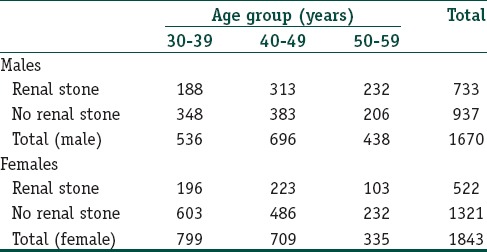
A χ² for trend analysis with this data returns a χ²_trend value of 49.70 which at df = 1 yields P < 0.001, indicating that the increasing trend in stone proportion with age is statistically highly significant and likely to be true.

Now, let us look at the same data rearranged with stratification by gender:

Now, for the male stratum, χ²_trend value is 31.73 (df = 1; P < 0.001), and for the female stratum, it is 7.14 (df = 1; P = 0.008). A Mantel-Haenszel analysis will however yield a composite χ²_trend value of 35.34 (df = 1; P < 0.001). Thus, we can interpret these results as a significant trend in stone proportion increase with age, overall as also separately for males and females. In this particular case, there is no confounding effect of gender.

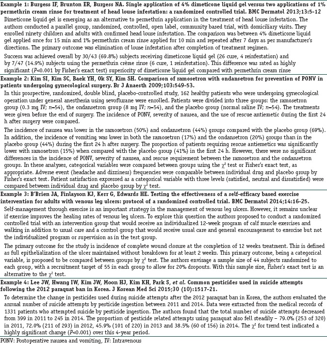
A Cochran–Mantel–Haenszel procedure follows a similar logic and is used to derive a composite interpretation for repeated tests of independence. It is commonly applied to a situation where we have multiple 2 × 2 tables summarizing independent proportions and these tables represent repeat sets of data such as obtained through experiments or observations repeated at different times. Thus, we are dealing with three categorical variables, the two that make up individual 2 × 2 tables and a third nominal variable that identifies the repetitions such as time, location, or study. In essence, a Mantel–Haenszel χ² statistic is calculated here also. In fact, the terms Cochran–Mantel–Haenszel test and Mantel–Haenszel test have been used interchangeably. This is confusing but not wrong considering that the basic idea of Cochran (1954) was modified by Mantel and Haenszel (1959) to derive the test formula. The Cochran–Mantel–Haenszel test has also been used to quantify the conclusion of meta-analyses dealing with multiple studies that look at the same binary outcome in two-arm trials. Box 1 provides some examples of comparison of independent proportions from published literature.

Box 1.

Examples of comparison of independent proportions from published literature

Chi-square Goodness-of-fit Test

This represents a different use of the χ² statistic. The test is applied in relation to a single categorical variable drawn from a population through random sampling. It is used to determine whether sample data are consistent with a hypothesized distribution in the population.

For example, suppose a pharmaceutical company has printed promotional cards which are being enclosed with packs of a new health drink. It claims that 20% of its cards are gold cards, 30% silver cards, and 50% bronze cards and these cards enable consumers to claim discounts (maximum for gold card) on purchase of the next pack. We could gather a random sample of these promotional cards, calculate the expected frequencies of each card category, and compare with the observed frequencies using a χ² goodness-of-fit test to see whether our sample distribution differs significantly from the distribution claimed by the company. A significant P value would mean we have to reject the null hypothesis of a good fit.

The χ² goodness-of-fit test is an alternative to the Anderson–Darling and Kolmogorov–Smirnov goodness-of-fit tests. It can be applied to discrete probability distributions such as the binomial and the Poisson. The Kolmogorov–Smirnov and Anderson–Darling tests are restricted to continuous distributions, for which they are actually more powerful.

Likelihood Ratio Chi-square Test

Likelihood ratio Chi-square test, also called the likelihood test or G test, is an alternative procedure to test the hypothesis of no association of columns and rows in a contingency table of nominal data. Although calculated differently, likelihood ratio χ² is interpreted in the same way as Pearson's χ². For large samples, likelihood ratio χ² will be close to Pearson χ². Even for smaller samples, it rarely leads to substantially different results if a continuity correction is applied and is therefore infrequently used.

McNemar's Chi-square Test

McNemar's χ² test (after Quinn McNemar, 1947), also simply called McNemar's test, assesses the difference between paired proportions. Thus, it is used when the frequencies in a 2 × 2 table represent paired (dependent) samples or observations. The null hypothesis is that the paired proportions are equal.

It is important to note that the layout of the contingency table for analyzing paired data is different from that used with unpaired samples. For paired data, a contingency table is created in one of the ways depicted in Table 3 depending on the nature of the data:

Table 3.

Data arrangement in two-dimensional contingency table for the McNemar's test

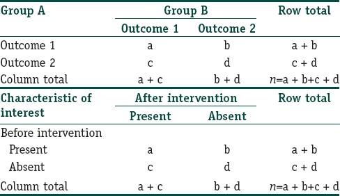
The calculation of the McNemar's χ² statistics is different from that described above for the Pearson's χ² test. The test involves calculating the difference between the number of discordant pairs in each category and scaling this difference by the total number of discordant pairs. The value of the McNemar's χ² is referred to the χ² distribution table with df 1.

An important observation when interpreting McNemar's test is that the elements of the concordant diagonal do not contribute to the decision about whether (in the above example) pre- or post-intervention condition is more favorable. Thus, the sum b + c can be small and statistical power of the test can be low even though total N is large. If either b or c is too small or b + c is <25, the traditional advice is not to use McNemar's test and instead use an alternative called the exact binomial test. If this is not feasible, Edwards continuity correction (after Allen Edwards) version of the McNemar's test can be used to approximate the binomial exact P value.

An extension of McNemar's test application is to situations where there are clusters of paired data where the pairs in a cluster may not be independent, but independence holds between different clusters. An example is analyzing the effectiveness of a dental procedure; in this case, a pair corresponds to the treatment of an individual tooth in patients who might have multiple teeth treated; the effectiveness of treatment of two teeth in the same patient is not likely to be independent, but the treatment of two teeth in different patients is more likely to be independent.

The sample size requirement sometimes specified for the McNemar's test is that the number of discordant pairs should be at least 10. For small samples, a continuity correction, as stated above, may be applied during the calculation if number of discordant pairs are small. However, the test cannot be applied to a larger than 2 × 2 table. In such a situation, Cochran's Q test may be used.

Exact versions of the McNemar's test that is similar to the Fisher's exact test have been devised but are yet to be readily available in computer software.

Cochran's Q Test

Cochran's Q test (after William Gemmell Cochran, 1950) is essentially a generalization of the McNemar's test that compares more than two related proportions. If there is no difference between the proportions, the test statistic Q has, approximately, a χ² distribution with (r − 1) df.

Although the test assumes random sampling, it is a nonparametric test and does not require normal distribution. The outcome is to be coded as binary responses with the same interpretation across categories. It should not be applied to small sample sizes. Since Cochran's Q test is for related samples, cases with missing observations for one or more of the variables are excluded from the analysis automatically by software which do the test.

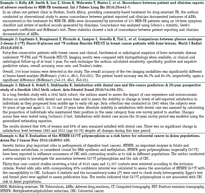
The Cochran's Q test is commonly used for assessing the hypothesis of no inter-rater difference in situations where a number of raters judge the presence or absence of some characteristic in a group of subjects. Box 2 provides examples of comparison of paired proportions from published literature.

Box 2.

Examples of comparison of paired proportions from published literature

Binomial Test and Sign Test

The binomial test is an exact test of the statistical significance of deviations from a theoretically expected distribution of observations into two categories, that is a binomial distribution. One common use of the binomial test is to test the null hypothesis that two “success or failure” type counts are equally likely to occur. For instance, suppose a dice is rolled 100 times and 6 is obtained 24 times. Since theoretically for an unbiased dice, 6 should appear 17 times, we can use the binomial test to decide if the observed count is significantly different from the expected count.

The binomial test has certain assumptions. There has to be a number of observations which is small compared to the possible number of observations. The observations are dichotomous, i.e., each observation will fall into one of just two categories. Individual observations are independent and the probability of “success” or “failure” is the same for each observation. For large samples, the binomial distribution is well approximated by continuous probability distributions, and these are used as the basis for alternative tests that are simpler such as the Pearson's χ² test or the G test. However, for small samples, these approximations break down, and the binomial test is a better choice. When the observations can fall in more than two categories, and an exact test is required, the multinomial test, based on the multinomial distribution, must be used instead of the binomial test.

The sign test is a special case of the binomial test where the probability of success under the null hypothesis is 0.5. It is used in repeated measurement designs that measure a categorical dependent variable on the same subjects before and after some intervention. It tests if the direction of change of counts is random or not. The change is expressed as a binary variable taking the value “+” if the dependent variable value following the intervention is larger than earlier and “−” if it is smaller. When there is no change, the change is coded 0 and is ignored in the analysis. When we consider this test, we are not focusing on the magnitude of the outcome but rather on its direction.

For example, suppose we measure the average number of cigarettes smoked daily by a group of 15 new smokers before and after they are exposed to counseling sessions on the dangers of smoking. After the intervention, out of these 15 individuals, 5 smoke the same number of cigarettes, 9 smoke less, and 1 smoke more. Can we consider that the counseling intervention diminished smoking tendency? This problem is equivalent to considering nine favorable outcomes against one unfavorable outcome with probability of outcome as 0.5. In this case, a sign test would yield P < 0.05 and we can conclude that counseling did change the smoking behavior favorably.

In clinical trials, the binomial test could be used to assess whether a single study site in a multicentric trial has the rate of a particular event similar to that observed in the entire study population. In epidemiology, this test can show whether observed prevalence in a sample matches the known prevalence in the population. Since the sign test is a statistical method to test for consistent differences between pairs of observations, it has been used to test the null hypothesis that the difference between the median of a numerical variable X and the median of another numerical variable Y is zero, assuming continuous distributions of the two variables X and Y, in the situation when we can draw paired samples from X and Y. It can also test if the median of a data set is significantly greater or less than a specified value.

Beyond the Chi-square Statistic in Comparing Categorical Variables between Groups

The χ² statistic is used to estimate whether or not a significant difference exists between groups with respect to categorical variables, but the P value, it yields does not indicate the strength of the difference or association.

This information can be obtained from the relative risk (risk ratio) or odds ratio. Both are measures of dichotomous association in that they are applied to 2 × 2 tables in such a way so as to measure the strength of relationships. These estimations are routinely used in epidemiological research where the relationship between exposure to risk factors and adverse outcomes needs to be studied. They are increasingly being used in interventional studies. These issues will be considered in the risk assessment module.

Financial support and sponsorship

Nil.

Conflicts of interest

There are no conflicts of interest.