Predictive Sampling of Rare Conformational Events in Aqueous Solution: Designing a Generalized Orthogonal Space Tempering Method

Abstract

In aqueous solution, solute conformational transitions are governed by intimate interplays of the fluctuations of solute-solute, solute-water, and water-water interactions. To promote essential fluctuations to enhance sampling, a common strategy is to construct an expanded Hamiltonian through a series of Hamiltonian perturbations, for instance on certain interactions of focus. Due to lack of active sampling of configuration response to perturbation transitions, it is challenging for common expanded Hamiltonian methods to robustly explore solvent mediated rare conformational events. The orthogonal space sampling (OSS) scheme, as exemplified by the orthogonal space random walk and orthogonal space tempering methods, provides a general framework for synchronous acceleration of slow configuration responses. To more effectively sample conformational transitions in aqueous solution, in this work, we devised a generalized orthogonal space tempering (gOST) algorithm. Specifically, in the Hamiltonian perturbation part, a solvent-accessible-surface-area-dependent term is introduced to implicitly perturb near-solute water-water fluctuations; and in the orthogonal space response part, the generalized force order parameter is generalized as a two-dimension order parameter set, in which the solute-solvent and solute-solute components are separately treated. The gOST algorithm is evaluated through a molecular dynamics simulation study on the explicitly-solvated deca-alanine (Ala₁₀) peptide. Based on a fully automated sampling protocol, the gOST simulation enabled repetitive folding and unfolding of the solvated peptide within a single continuous trajectory and allowed for detailed constructions of Ala₁₀ folding/unfolding free energy surfaces. The gOST result reveals that solvent cooperative fluctuations play a pivotal role in Ala₁₀ folding/unfolding transitions. In addition, our assessment analysis suggests that because essential rare events are mainly driven by the compensating fluctuations of the solute-solvent and solute-solute interactions, commonly employed “predictive” sampling methods are unlikely to be effective on this seemingly “simple” system. The gOST development presented in this paper illustrates the power of the OSS scheme for physics-based sampling method designs.

Introduction

Governed by the intimate interplays of solute-solute, solute-water, and water-water interactions, solute molecules in aqueous solution constantly fluctuate. Critical fluctuations, when reaching adequate amplitudes, can drive significant conformational transitions. Understanding conformational changes in aqueous solution has been a key topic in the field of biomolecular simulation. For the fact that many biomolecular processes are beyond timescales that canonical ensemble molecular dynamics (MD) can routinely reach, specialized sampling techniques are of great importance.

The past decades have observed the flourishing of enhanced-sampling method developments. An important aspect of these efforts is to develop predictive sampling methods that do not rely on specific prior knowledge. A general strategy is to construct an expanded Hamiltonian through a series of perturbed Hamiltonians, as is exemplified by temperature/Hamiltonian replica exchange (TREM/HREM) and simulated tempering/scaling (ST/SS) methods etc., thereby to enlarge the fluctuations of pre-chosen interactions. Taking the potential scaling scheme (as represented by the HREM and SS methods) as the example, the general expanded Hamiltonian can be expressed as

$$H_{\lambda }=\lambda U_{\mathit{\text{ss}}}\left({\mathit{X}}_{\mathit{N}}\right)+SE\left(\lambda \right)U_{se}\left({\mathit{X}}_{\mathit{N}}\right)+U_e\left({\mathit{X}}_{\mathit{N}}\right)+{\sum }_{\mathit{i}=1}^N{{\mathit{p}}_i}^2/2m_i+{p_{\lambda }}^2/2m_{\lambda },$$ (1)

where U_ss(X_N) and U_se(X_N) respectively represent selected solute-solute and solute-solvent interactions that are subject to the scaling perturbation treatment; and U_e(X_N) represents the remaining “environmental” interactions. To be general, while U_ss(X_N) is straightly scaled by a factor λ, U_se(X_N) is scaled by a pre-chosen λ-dependent function SEλ. The λ-space dynamics can be realized through either hybrid Monte Carlo (MC) based methods or the extended dynamics approach, the latter of which requires the scaling factor λ to be treated as a one-dimension particle with the kinetic energy of p_λ²/2m_λ. To enable random and broad visits of pre-chosen λ states, one usually needs to introduce a biasing potential function f_m(λ) (for the extended MC scheme, correspondingly a biasing weight function) or utilize the MC-based replica exchange technique. In comparison with “global” sampling methods like TREM and ST, such potential-scaling-based “focusing” sampling approaches allow fluctuation promotions to be selectively concentrated on essential interactions and thus allow possible diffusion sampling overheads to be reduced.

In the past decades, the potential-scaling-based expanded Hamiltonian strategy has attracted tremendous interest. As is increasingly known, applying such methods to explore rare conformational events in aqueous solution is not readily trivial, even on systems with moderate complexities. Indeed although varying λ may lead to a shifted distribution, it can take very long time for a configuration to dynamically evolve so as to realize the distribution change; i.e. slow configuration responses (to λ transitions), particularly ones involving across-barrier transitions, are likely to be the major sampling bottleneck. To tackle this configuration “lagging” issue, which in the context of free energy simulation is also called the “hidden free energy barrier” problem, we introduced the orthogonal space sampling (OSS) scheme, as exemplified by the orthogonal space random walk (OSRW) and orthogonal space tempering (OST) methods. To enable the corresponding OST sampling, the expanded Hamiltonian needs to be further modified as the following:

$$H_m=H_{\lambda }+f_m(\lambda )+\alpha g_m(\lambda ,F_{\lambda }),$$ (2)

in which H_λ corresponds to the one in Equation 1; to achieve λ space random walks, the target function of f_m(λ) is set as −G_o(λ), the negative of the λ-dependent free energy function under the H_λ ensemble; and to synchronously accelerate configuration responses, the target function of g_m(λ,F_λ) is set as −G_f(λ,F_λ), the negative of the free energy function along (λ,F_λ) under the H_o(λ) ensemble. In OST, the generalized force F_λ, specifically defined as ∂H_λ/∂λ, is applied as the response order parameter. Here, the parameter α controls the magnitude of response fluctuation enlargement; when α is equal to one, the OST method turns to the OSRW method. It is worth noting that α can be expressed as $\frac{T_{ES}-T_o}{T_{ES}}$, where T_o is the system reservoir temperature and T_ES is called the orthogonal space sampling temperature because at each the H ensemble, the F_λ distribution is proportional to $e\frac{G_f(\lambda ,F_{\lambda })}{k{T}_{ES}}$.

As is previously noted, the original OSS treatment can only robustly accelerate strongly coupled response fluctuations. In the context of the expanded Hamiltonian sampling, its performance is highly sensitive to the specific form of the scaling function SE(λ), which unfortunately needs to be empirically chosen; for instance, with the general condition of “SE(1)=1”, commonly employed functional forms include λ, (λ + 1)/2, and $\sqrt{\lambda }$ etc. As one can tell from Equation 1, SE(λ) governs how different interactions, including un-scaled solvent-solvent interactions, dynamically interplay at different perturbed states. More to note, the response order parameter F_λ in Equation 2 is specifically defined as $U_{\mathit{\text{ss}}}\left({\mathbf{X}}_{\mathit{N}}\right)+\frac{\mathit{\text{dSE}}\left(\lambda \right)}{d\lambda }{U}_{se}\left({\mathbf{X}}_{\mathit{N}}\right)$; it has no direct solvent-solvent contribution but two solute related components, between which the ratio is strictly SE(λ) dependent. As discussed in our early study, along different microscopic events, the relative fluctuations between U_ss (X_N) and U_se (X_N) may follow drastically distinct directions. The actual relative fluctuation directions may not be in good accord with their ratio $(1:\frac{\mathit{\text{dSE}}\left(\lambda \right)}{d\lambda })$ in the response order parameter function F_λ. Therefore effective activation of slow essential response events cannot be guaranteed by the original OST treatment. In this work, to more robustly accelerate configuration responses in aqueous environments, we devised a generalized orthogonal space tempering (gOST) algorithm. Specifically, in the Hamiltonian perturbation part, besides a common potential scaling treatment, a solvent-accessible-surface-area-dependent term is introduced to implicitly perturb near-solute water-water fluctuations; and in the orthogonal space response part, the response order parameter is generalized as a two-dimension order parameter set, where the SE(λ)-dependent solute-solvent term is separately treated. Through these generalization treatments, first, water-water response fluctuations can be actively accelerated; and second, irrespective of the function form chosen for SE(λ), response fluctuations of both the essential solute-solute and solute-solvent interactions can be robustly promoted.

The new gOST algorithm was evaluated through a molecular dynamics simulation study on the explicitly-solvated deca-alanine (Ala₁₀) peptide. Based on a fully automated sampling protocol, the gOST simulation enabled repetitive folding and unfolding of the solvated peptide and allowed for detailed constructions of Ala₁₀ folding/unfolding free energy surfaces. The gOST result reveals that solvent cooperative fluctuations play a pivotal role in Ala₁₀ folding/unfolding transitions. In addition, our assessment analysis suggests that because the rare events are mainly driven by the compensating fluctuations of the solute-solvent and solute-solute interactions, most current sampling methods are unlikely to be effective on this seemingly simple system. The gOST development presented in this paper illustrates the power of the OSS scheme for physics-based predictive sampling method designs.

Theoretical Design

In this section, we first summarize the original orthogonal space tempering (OST) method, then introduce the new generalized orthogonal space tempering (gOST) algorithm, and finally describe how to construct free energy surfaces based on samples collected from gOST simulations.

Brief Introduction to the Orthogonal Space Tempering (OST) Method

The OST algorithm is an adaptive sampling method. To recursively generate the target biasing potentials, an extended-dynamics based “double-integration” recursion strategy was developed. To do so, the target OST Hamiltonian in Equation 2 needs to be modified as follows:

$$H_m=H_{\lambda }+\frac{{p_{\varphi }}^2}{2m_{\varphi }}+ \frac{1}{2}{K}_{\varphi }{(\frac{\partial H_{\lambda }}{\partial \lambda }-\varphi )}^2+f_m\left(\lambda \right)+\alpha g_m\left(\lambda ,\varphi \right),$$ (3)

in which by introducing an additional fictitious particle ϕ, we extend the expanded Hamiltonian H_λ in Equation 1 to $H_{\varphi }=H_{\lambda }+\frac{{p_{\varphi }}^2}{2m_{\varphi }}+ \frac{1}{2}{K}_{\varphi }{(\frac{\partial H_{\lambda }}{\partial \lambda }-\varphi )}^2$; here through the restraint tertm, $\frac{1}{2}{K}_{\varphi }{(\frac{\partial H_{\lambda }}{\partial \lambda }-\varphi )}^2$, ϕ can play a role as the dynamic restraining reference (DRR) of $\frac{\partial H_{\lambda }}{\partial \lambda }$. The same as the scaling factor λ, the DDR variable ϕ is treated as a one-dimension particle with a mass of m_ϕ In OST, the extended particles, λ and ϕ, are propagated based on independent Langevin dynamics equations, the temperatures in which are set as the same as the system reservoir temperature T_o.

To realize the “double-integration” recursion, for each λ′ state, g_m(λ′, ϕ) can be adaptively evaluated via an adaptive biasing force (ABF) like procedure, specifically based on the following equation:

$$g_m\left(\lambda \text{'},\varphi \right)=-{\int }_{{\varphi }_{\mathit{\text{min}}}\left({\lambda }^{\prime }\right)}^{\varphi }{\langle \frac{\partial H_{\varphi }}{{\partial }_{\varphi }}}_{\lambda ’}\rangle d\varphi +C_{g_m}\left(\lambda \text{'}\right),$$ (4)

where the integration is carried out within the dynamically evolving boundary [ϕ_min(λ′), ϕ_max(λ′)]; and the calibration constant C_gm (λ′) is calculated as follows:

$$C_{g_m}\left(\lambda \text{'}\right)=-\mathit{\text{max}}[g_m\left(\lambda \text{'},\varphi \right)]-k{T}_{o}ln{\int }_{{\varphi }_{\mathit{\text{min}}}\left({\lambda }^{\prime }\right)}^{{\varphi }_{\mathit{\text{max}}}\left({\lambda }^{\prime }\right)}\mathit{\text{exp}}\left(\frac{g_m\left({\lambda }^{\prime },\varphi \right)-\mathit{\text{max}}\left[g_m\left({\lambda }^{\prime },\varphi \right)\right]}{k{T}_o}\right)d\varphi .$$ (5)

Then the two-dimension function g_m(λ, ϕ) can be generated via the assembling of the calculated one-dimension g_m(λ′, ϕ) functions. Furthermore, we can adaptively acquire f_m(λ) through another integration calculation:

$$f_m\left(\lambda \right)=-{\int }_{{\lambda }_{\mathit{\text{min}}}}^{\lambda }\frac{{\int }_{{\varphi }_{\mathit{\text{max}}}\left({\lambda }^{\prime }\right)}^{{\varphi }_{\mathit{\text{min}}}\left({\lambda }^{\prime }\right)}\varphi \mathit{\text{exp}}\left(\frac{g_m\left({\lambda }^{\prime },\varphi \right)}{k{T}_o}\right)d\varphi }{{\int }_{{\varphi }_{\mathit{\text{max}}}\left({\lambda }^{\prime }\right)}^{{\varphi }_{\mathit{\text{min}}}\left({\lambda }^{\prime }\right)}\mathit{\text{exp}}\left(\frac{g_m\left({\lambda }^{\prime },\varphi \right)}{k{T}_o}\right)d\varphi }d\lambda \text{'}.$$ (6)

It is noted that for OST free energy calculations, an extra correction operation is required to obtain accurate G_o(λ); for predictive sampling, the above equation should be adequate.

Generalized Orthogonal Space Tempering (gOST) Method

As discussed earlier, in gOST, two major changes are made from the original OST method. First, a solvent-accessible-surface-area-dependent term, [SASA(λ) – 1] U_sasa (X_N), is introduced to construct a new expanded Hamiltonian:

$$H_{\lambda }=\lambda U_{\mathit{\text{ss}}}\left({\mathit{X}}_{\mathit{N}}\right)+SE\left(\lambda \right)U_{se}\left({\mathit{X}}_{\mathit{N}}\right)+\left[\mathit{\text{SASA}}\left(\lambda \right)-1\right]U_{\mathit{\text{SASA}}}\left({\mathit{X}}_{\mathit{N}}\right)+U_e\left({\mathit{X}}_{\mathit{N}}\right)+{\sum }_{\mathit{i}=1}^N{{\mathit{P}}_i}^2/2m_i+{{\mathrm{p}}_{\lambda }}^2/2m_{\lambda },$$ (7)

where U_sasa (X_N) represents the solvent accessible surface area (SASA) energy that is commonly used to model non-polar solvation contributions and sasa (λ) is the corresponding scaling function with the condition of SASA(1) = 1. This SASA term plays two inter-related roles: (1) it can effectively vary the surface tension surrounding the solute molecule and so indirectly perturbs near-solute solvent-solvent interactions; (2) correspondingly in the response order parameter F_λ, there is an additional $\frac{d\mathit{\text{SASA}}\left(\lambda \right)}{d\lambda }{U}_{\mathit{\text{SASA}}}\left({\mathit{X}}_{\mathit{N}}\right)$ term that allows near-solute solvent-solvent fluctuations to be indirectly accelerated through the OSS treatment.

Second, we generalize the response order parameter $F_{\lambda }\left[U_{\mathit{\text{ss}}}\left({\mathit{X}}_{\mathit{N}}\right)+\frac{\mathit{\text{dSE}}\left(\lambda \right)}{d\lambda }{U}_{se}\left({\mathit{X}}_{\mathit{N}}\right)+\frac{d\mathit{\text{SASA}}\left(\lambda \right)}{d\lambda }{U}_{\mathit{\text{SASA}}}\left(X_N\right)\right]$ to a two-dimension response order parameter set $\left(F_{\lambda }^{\mathit{\text{intra}}},F_{\lambda }^{\mathit{\text{inter}}}\right)$, where $F_{\lambda }^{\mathit{\text{intra}}}$ denotes $U_{\mathit{\text{ss}}}\left({\mathit{X}}_{\mathit{N}}\right)+\frac{d\mathit{\text{SASA}}\left(\lambda \right)}{d\lambda }{U}_{\mathit{\text{SASA}}}\left({\mathit{X}}_{\mathit{N}}\right)$; and $F_{\lambda }^{\mathit{\text{inter}}}$ denotes $\frac{\mathit{\text{dSE}}\left(\lambda \right)}{d\lambda }{U}_{se}\left({\mathit{X}}_{\mathit{N}}\right)$. As discussed in our previous study, following microscopic events, solute-solute and solute-solvent interactions may have distinct interplays and often fluctuate in a compensating manner; therefore separately treating them through a two-dimension order parameter set can lead to more robust activation of their fluctuations. Generalized from Equation 2, the gOST Hamiltonian should be expressed as

$$H_m=H_{\lambda }+f_m\left(\lambda \right)+\alpha g_m\left(\lambda ,F_{\lambda }^{\mathit{\text{intra}}},F_{\lambda }^{\mathit{\text{inter}}}\right),$$ (8)

in which H_λ is the same as in Equation 7 and the target function of $g_m\left(\lambda ,F_{\lambda }^{\mathit{\text{intra}}},F_{\lambda }^{\mathit{\text{inter}}}\right)$ is set as $-G_f\left(\lambda ,F_{\lambda }^{\mathit{\text{intra}}},F_{\lambda }^{\mathit{\text{inter}}}\right)$, the negative of the free energy function along $\left(\lambda ,F_{\lambda }^{\mathit{\text{intra}}},F_{\lambda }^{\mathit{\text{inter}}}\right)$ under the ensemble of H_λ – G_o(λ). To realize the double-integration recursion, the gOST Hamiltonian needs to be further modified as

$$H_m=H_{\lambda }+\frac{{p_{{\varphi }_1}}^2}{2m_{{\varphi }_1}}+\frac{{p_{{\varphi }_2}}^2}{2m_{{\varphi }_2}}+\frac{1}{2}{K}_{{\varphi }_1}{(F_{\lambda }^{\mathit{\text{intra}}}-{\varphi }_1)}^2+\frac{1}{2}{K}_{{\varphi }_2}{(F_{\lambda }^{\mathit{\text{inter}}}-{\varphi }_2)}^2+f_m\left(\lambda \right)+\alpha g_m\left(\lambda ,F_{\lambda }^{\mathit{\text{intra}}},F_{\lambda }^{\mathit{\text{inter}}}\right),$$ (9)

in which instead of ϕ, we introduced two extended particles, ϕ₁ and ϕ₂. Then the H_λ Hamiltonian in Equation 7 is generalized to a new Hamiltonian: $H_{{\varphi }_1,{\varphi }_2}=H_{\lambda }+\frac{{p_{{\varphi }_1}}^2}{2m_{{\varphi }_1}}+\frac{{p_{{\varphi }_2}}^2}{2m_{{\varphi }_2}}+\frac{1}{2}{K}_{{\varphi }_1}{(F_{\lambda }^{\mathit{\text{intra}}}-{\varphi }_1)}^2+\frac{1}{2}{K}_{{\varphi }_2}{(F_{\lambda }^{\mathit{\text{inter}}}-{\varphi }_2)}^2$. Different from ϕ in the original OST recursion, which serves as a dynamic restraining reference, here, ϕ₁ and ϕ₂ are designed to serve as adaptive dynamic reporters (ADRs). Specifically during each recursion, we adaptively generate g_m(λ, ϕ_1, ϕ₂), whereas during each energy calculation and dynamic propagation, we use $F_{\lambda }^{\mathit{\text{intra}}}$ and $F_{\lambda }^{\mathit{\text{inter}}}$ instead of ϕ₁ and ϕ₂ as the respective variables. As for the “double-integration” recursion, for each λ′ state, we can obtain g_m(λ′, ϕ₁, ϕ₂) via the following path integration

$$g_m({\lambda }^{\prime },{\varphi }_1,{\varphi }_2)=-{\oint }_{[{\varphi }_{1,\mathit{\text{min}}}\left({\lambda }^{\prime }\right),{\varphi }_{2,\mathit{\text{min}}}\left({\lambda }^{\prime }\right)]}^{({\varphi }_{1,}{\varphi }_2)}{\langle \frac{\partial H_{{\varphi }_1,{\varphi }_2}}{\partial \mathit{\Phi }}\rangle }_{\lambda ’}d\mathit{r}+C_{g_m}\left({\lambda }^{\prime }\right),$$ (10)

in which ${\langle \frac{\partial H_{{\varphi }_1,{\varphi }_2}}{\partial \mathit{\Phi }}\rangle }_{\lambda }$, denotes $\left({\langle \frac{\partial H_{{\varphi }_1,{\varphi }_2}}{\partial {\varphi }_1}\rangle }_{{\lambda }^{\prime }},{\langle \frac{\partial H_{{\varphi }_1,{\varphi }_2}}{\partial {\varphi }_2}\rangle }_{{\lambda }^{\prime }}\right)$, a (ϕ₁, ϕ₂) space vector; and r represents a possible (ϕ₁, ϕ₂) space pathway between [ ϕ₁(λ′), ϕ₂(λ′)] and ϕ₁, ϕ₂. Following the strategy in a recent ABF implementation, the Monte-Carlo integration method was used to calculate ${\oint }_{[{\varphi }_{1,\mathit{\text{min}}}\left({\lambda }^{\prime }\right),{\varphi }_{2,\mathit{\text{min}}}\left({\lambda }^{\prime }\right)]}^{({\varphi }_{1,}{\varphi }_2)}{\langle \frac{\partial H_{{\varphi }_1,{\varphi }_2}}{\partial \mathit{\Phi }}\rangle }_{\lambda ’}d\mathit{r}$; this allows us to take into account of all the possible pathways in a maximum likelihood manner. Generalizing Equation 5, we have the following equation to calculate the calibration constant C_gm:

$$C_{g_m}\left({\lambda }^{\prime }\right)=-\mathit{\text{max}}[g_m({\lambda }^{\prime },{\varphi }_1,{\varphi }_2)]-k{T}_{o}ln{\iint }_{[{\varphi }_{1,\mathit{\text{min}}}\left({\lambda }^{\prime }\right),{\varphi }_{2,\mathit{\text{min}}}\left({\lambda }^{\prime }\right)]}^{[{\varphi }_{1,\mathit{\text{max}}}\left({\lambda }^{\prime }\right),{\varphi }_{2,\mathit{\text{max}}}\left({\lambda }^{\prime }\right)]}\mathit{\text{exp}}\left(\frac{g_m\left({\lambda }^{\prime },{\varphi }_1,{\varphi }_2\right)-\mathit{\text{max}}[g_m\left({\lambda }^{\prime },{\varphi }_1,{\varphi }_2\right)]}{k{T}_o}\right)d{\varphi }_{1}d{\varphi }_2.$$ (11)

Then the target three-dimension function g_m(λ, ϕ₁, ϕ₂) can be directly assembled from the calculated two-dimension g_m(λ′, ϕ₁, ϕ₂) functions. Generalizing Equation 6, we have the following equation to adaptively calculate f_m(λ):

$$-{\int }_{{\lambda }_{\mathit{\text{min}}}}^{\lambda }\left(\frac{{\int }_{{\varphi }_{1,\mathit{\text{min}}}({\lambda }^{\prime })}^{{\varphi }_{1,\mathit{\text{max}}}({\lambda }^{\prime })}{\varphi }_1{\int }_{{\varphi }_{2,\mathit{\text{min}}}({\lambda }^{\prime })}^{{\varphi }_{2,\mathit{\text{max}}}({\lambda }^{\prime })}\mathit{\text{exp}}\left(\frac{g_m({\lambda }^{\prime },{\varphi }_1,{\varphi }_2)}{k{T}_o}\right)d{\varphi }_{2}d{\varphi }_1}{{\int }_{{\varphi }_{1,\mathit{\text{min}}}({\lambda }^{\prime })}^{{\varphi }_{1,\mathit{\text{max}}}({\lambda }^{\prime })}{\int }_{{\varphi }_{2,\mathit{\text{min}}}({\lambda }^{\prime })}^{{\varphi }_{2,\mathit{\text{max}}}({\lambda }^{\prime })}\mathit{\text{exp}}\left(\frac{g_m({\lambda }^{\prime },{\varphi }_1,{\varphi }_2)}{k{T}_o}\right)d{\varphi }_{2}d{\varphi }_1}+\frac{{\int }_{{\varphi }_{2,\mathit{\text{min}}}({\lambda }^{\prime })}^{{\varphi }_{2,\mathit{\text{max}}}({\lambda }^{\prime })}{\varphi }_2{\int }_{{\varphi }_{1,\mathit{\text{min}}}({\lambda }^{\prime })}^{{\varphi }_{1,\mathit{\text{max}}}({\lambda }^{\prime })}\mathit{\text{exp}}\left(\frac{g_m({\lambda }^{\prime },{\varphi }_1,{\varphi }_2)}{k{T}_o}\right)d{\varphi }_{2}d{\varphi }_1}{{\int }_{{\varphi }_{2,\mathit{\text{min}}}({\lambda }^{\prime })}^{{\varphi }_{2,\mathit{\text{max}}}({\lambda }^{\prime })}{\int }_{{\varphi }_{1,\mathit{\text{min}}}({\lambda }^{\prime })}^{{\varphi }_{1,\mathit{\text{max}}}({\lambda }^{\prime })}\mathit{\text{exp}}\left(\frac{g_m({\lambda }^{\prime },{\varphi }_1,{\varphi }_2)}{k{T}_o}\right)d{\varphi }_{2}d{\varphi }_1}\right)d{\lambda }^{\prime }.$$ (12)

The same as Equation 6, Equation 12 is an approximate way of estimating f_m(λ); however it is sufficient for the purpose of predictive sampling.

Generalized Orthogonal Space Tempering Simulation Result Analysis

For any collective variable set S of interest, the free energy surface can be constructed based on the following equation,

$$G_o\left(\mathit{S}\right)=-k{T}_{o}ln{\sum }_t{e}^{\frac{H_m\left(t\right)-H_o\left(t\right)}{k{T}_o}}\delta \left(\mathit{S}[{\mathit{X}}_{\mathit{N}}\left(t\right)]-\mathit{S}\right)+ \mathit{\text{constant}},$$ (13)

where t represents scheduled sample-collection time-steps in the near-equilibrium phase of the simulation. The above extended-ensemble-to-canonical-ensemble re-weighting strategy has been employed in our earlier OSS based simulation ^17,20 and on-the-path random walk based simulation studies²¹. It is a generalized form of the umbrella sampling formula¹³, which was originally derived in the canonical-ensemble-to-canonical-ensemble reweighting framework.

Computational Details

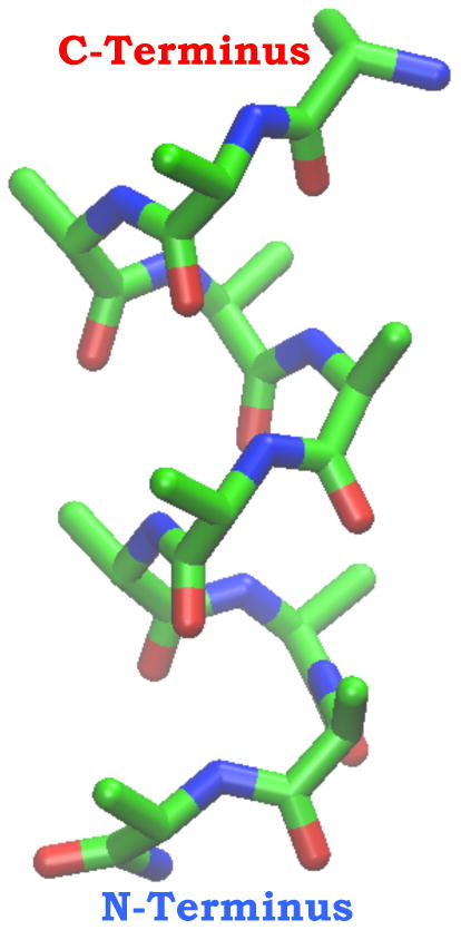
To test the gOST method, the explicitly-solvated deca-alanine (Ala₁₀) peptide (Figure 1) was chosen as the model system. Although Ala₁₀ is one of the most commonly studied systems, as far as we know, before this work, there has been no report on achieving “predictive” simulation of repetitive unfolding/refolding of the explicitly solvated Ala₁₀, in particular through a single continuous trajectory. As the matter of the fact, based on the gOST simulation result, our analysis suggests that commonly employed “predictive” sampling methods may not be very effective on this seemingly simple system.

Figure 1.

Calculated free energy potentials and it target potential for the “butane-like” molecule used in model system 1. The dash-dot curve shows the calculated free energy potential from a 1.2 ns classical metadynamics simulation using a low fixed Gaussian height (0.01 kcal/mol); the black solid curve shows the calculated free energy potential from a 1.2 ns classical metadynamics simulation using a large fixed Gaussian height (0.1 kcal/mol); the curve with open circles shows the calculated free energy potential from a 1.2 ns metadynamics simulation employing the Wang-Landau recursion; and the gray solid curve represents the target free energy potential.

Model and General Molecular Dynamics Simulation Setups

In the model, we have a deca-alanine peptide chain (Figure 1) solvated in a truncated octahedral water box; potassium and chloride ions were added to have the ionic strength adjusted around 0.15 M. The deca-alanine peptide and ions were modeled with the CHARMM22/CMAP force field and water molecules are treated with the modified TIP3P model. The particle mesh Ewald (PME) method²⁷ was used to treat long-range electrostatic interactions; in real space energy and force calculations, short-range electrostatic interactions were switched off at 12 Å. All the simulations were performed under the NPT ensemble. The temperature was set as 300 K and the pressure was set as 1 atm; the Nóse-Hoover thermostat²⁵ was utilized to maintain the constant temperature and the Langevin piston algorithm²⁶ was employed to maintain the constant pressure. The SHAKE algorithm was used to constrain all the bonds that involve water hydrogen atoms. The MD simulation time step was set as 1 femto-second (fs).

Details on the Generalized Orthogonal Space Tempering Simulation

The gOST algorithm was implemented in our customized version of the CHARMM program^28,29. In this study, we selected all the intra-peptide torsional (including the CMAP) and electrostatic energy terms into U_ss(X_N) and all the electrostatic interactions between the peptide and the solvent environment (including both water molecules and ions) into U_se(X_N); in the RESULTS AND DISCUSSION section, these energy components are respectively denoted as U_pp and U_pw. For SE(λ), we picked $\sqrt{\lambda }$ for no particular reason other than that it is a commonly employed functional form. For U_sasa(X_N), we used a surface-accessible-surface-area energy form in the CHARMM program. We collected experimentally determined temperature-dependent water surface tension changes γ(T_m) and set SASA(λ) as a B-spline function connecting the collected-points based on the relationship $\text{SASA}\left(\lambda \right)=\gamma \left(\frac{300K}{{\lambda }^2}\right)/\gamma \left(300K\right)$.

To constrain λ within our pre-set range [0.801, 1.001], following the original OST method, a θ-dynamics strategy was used. Specifically, we explicitly propagate a θ particle that travels periodically between −π and π; here, θ is the variable of the λ_m(θ) function: λ_m(θ) = λ_min + (λ_max − λ_min)λ(θ), in which λ(θ) takes the functional form as in the original OST method. Considering this θ-dynamics element, the expanded Hamiltonian in Equation 7 should be:

$$H_{\lambda }={\lambda }_m\left(\theta \right)U_{\mathit{\text{ss}}}\left({\mathit{X}}_{\mathit{N}}\right)+SE\left({\lambda }_m\left(\theta \right)\right)U_{se}\left({\mathit{X}}_{\mathit{N}}\right)+[\mathit{\text{SASA}}\left({\lambda }_m\left(\theta \right)\right)-1]U_{\mathit{\text{sasa}}}\left({\mathit{X}}_{\mathit{N}}\right)+U_e\left({\mathit{X}}_{\mathit{N}}\right)+{\sum }_{\mathit{i}=1}^N{{\mathbf{P}}_i}^2/2m_i+{{\mathrm{p}}_{\theta }}^2/2m_{\theta }$$ (14)

In our gOST simulation, the orthogonal space sampling temperature T_ES was set to 3000 K, corresponding to α = 0.9; the masses of the fictitious particles θ, ϕ₁, and ϕ₂ were respectively set as 2000, 0.0002, and 0.0002 atomic mass unit (amu); the restraint force constants K_ϕ1 and K_ϕ2 were set as 0.1 kcal^-1mol^-1. During gOST recursions, both f_m(λ) and ${\mathrm{g}}_{\mathrm{m}}\left(\lambda ,{\mathrm{F}}_{\lambda }^{\text{intra}},{\mathrm{F}}_{\lambda }^{\text{inter}}\right)$ were updated every 1 picosecond (ps). The trajectories were saved every 1.0 pico-second (ps) for post-processing analysis. For all the analysis based on Equation 13, only the data after 60 nano-seconds (ns) was used; here the first 60 ns portion of the simulation serves to equilibrate the system and generate converged biasing energy functions.

Results and Discussion

The gOST Simulation Enabled Repetitive Ala₁₀ Unfolding and Refolding

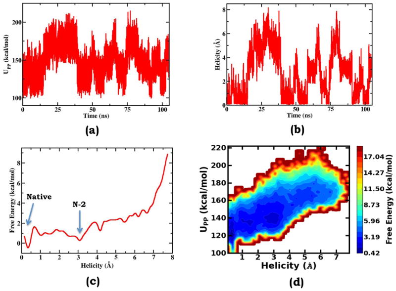
As shown in Figure 2a, during the gOST simulation, U_pp, the essential intra-solute energy, which serves as an independent term in the scaling perturbation treatment, fluctuates across several distinct regions. Each of these regions is featured with the corresponding enduring fluctuations and is connected with its neighboring regions through rare transitions. To characterize the conformation corresponding to each of these U_pp regions, based on our detailed survey of the trajectory, we defined a helicity deviation collective variable, $\sqrt{\frac{{\sum }_{i=6}^{i=1}{\left(d_i-3.0\right)}^2}{6}}$, in which d_i represents α-helix hydrogen bond distances. As comparatively shown, the fluctuation of the helicity deviation collective variable (Figure 2b) is intimately synchronous with the fluctuation of U_pp (Figure 2a). Specifically, the lowest U_pp region corresponds to the folded state with the lowest helicity deviation, the highest U_pp region corresponds to the unfolded states with the highest helicity deviation values, and the intermediate U_pp regions correspond to different degrees of partially unfolded conformations. The close correlation between the helicity deviation and the essential intra-solute interaction U_pp can be directly revealed by the free energy surface along these two collective variables (Figure 2d). It should be noted that in this study, all the free energy surfaces were generated based on the reweighting formula of Equation 13. In the gOST method, U_pp, labeled as $F_{\lambda }^{\mathit{\text{intra}}}$ in Equation 9, is employed as an independent response order parameter; the excellent correspondence between its fluctuations and essential conformational transitions clearly demonstrate the advantage of the generalization treatment in the gOST formulation.

Figure 2.

Model system 2 on the calculation of free energy potential along the distance between one methyl thiolate sulfur atom and the Zinc center, with which four methyl thiolates are coordinated. Zinc atom is colored in blue; carbon atoms are colored in green; sulfur atoms are colored in yellow; oxygen atom are colored in red; and hydrogen atoms are colored in white.

Further based on Equation 13, we constructed the one-dimension free energy surface along the helicity deviation collective variable (Figure 2c). The free energy surface displays multiple minima with the global one corresponding to the native α-helical state. In the region with the helicity deviation lower than 4.0 Å, each of the local minima can be identified to correspond to a partially unfolded state. For instance around 3.1 Å, the second lowest free energy minimum represents the state that has lost the two N-terminus end helical hydrogen bonds; here, this state is labeled as “N-2”. In regions with larger helicity deviation values, the conformational states are likely degenerate. Therefore it is difficult to assign individual states directly from the one-dimension free energy surface. Overall, the helicity deviation is an excellent order parameter to describe Ala₁₀ folding/unfolding transitions. We would like to note that in the following, we label various conformational states using symbols such as “N-l”, “C-m”, or “N-l/C-m”; taking the “N-l/C-m” as the example, it denotes the partially-unfolded state that loses l numbers of hydrogen bonds at the N-terminus end and m numbers of hydrogen bonds at the C-terminus end. Here, we define 3.45 Å as the cutoff value for the forming and breaking of an α-helical bond.

In our model, the CHARMM22/CMAP potential is used as the energy function. As is generally known, this energy function over-stabilizes the helical state and cannot model commonly expected cooperative folding/unfolding transitions. Our result agrees well with these general understanding. Specifically, our result shows that the CHARMM22/CMAP force field over-stabilizes some of the partially unfolded states, such as the “N-2” state; therefore it favors step-wise rather than concerted folding/unfolding pathways. Clearly, this commonly used protein force field is not appropriate for modeling peptide helix-coil transitions. However, because CHARMM22/CMAP features a more rugged energy surface than the actual physical one, this Ala₁₀ model imposes a greater sampling challenge and it can arguably serve as an ideal model system to evaluate sampling techniques. As far as we know, before this work, there has been no report on achieving repetitive unfolding/refolding of the explicitly solvated Ala₁₀, in particular through a single continuous trajectory. Based on the fact that in this study, the gOST method enabled successful exploration of a presumably more rugged energy landscape, we expect it to be more effective when more accurate force fields are applied to the solvated Ala₁₀ system.

The Classical End-to-End Distance is A Poor Collective Variable

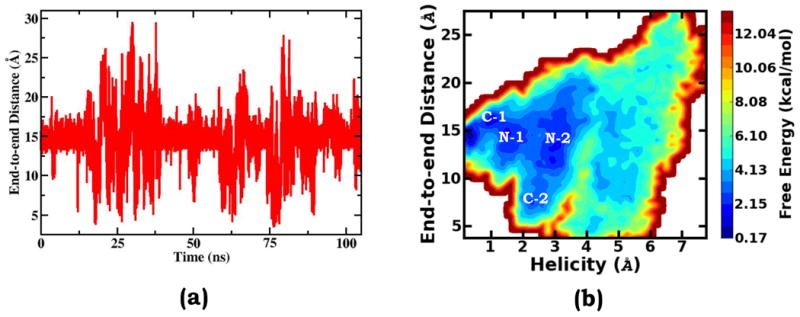
To analyze helix-coil transitions, the end-to-end distance is the most commonly employed order parameter. As shown by many earlier studies, fluctuations of this collective variable can closely follow Ala₁₀ gas phase folding/unfolding transitions and be an effective sampling order parameter. For the fact that in our gOST simulation study, no system-specific collective variable was applied to bias the sampling, the end-to-end distance can be evaluated in an unbiased manner. As comparatively shown in Figures 3a and 2b, the end-to-end distance does not monotonically change with each folding or unfolding transition. Instead, independent of the conformational region being visited, it mostly fluctuates up and down around 14.8 Å, the end-to-end distance of the native helical structure. Interestingly, the fluctuation range of the end-to-end distance has some degree of correlation with the conformational state. At the folded helical state, the fluctuation range is smaller, at the fully unfolded states, the fluctuation ranges are much larger, and at partially folded states, the fluctuation has intermediate magnitudes. Such correlation reflects the fact that unfolded regions of the peptide are very flexible and do not particularly prefer more extended conformations as they do in the gas phase. This can be further revealed by the two-dimensional free energy surface as the function of the helicity deviation and the end-to-end distance. Along the end-to-end distance direction, the free energy profile displays a largely pseudo-symmetric shape with 14.8 Å as the symmetry center. At the states of “N-1” and “N-2”, disordered N-terminus fragments by and large evenly fluctuate between extended and compact configurations. As the exception, when the partial unfolding occurs in the C-terminus end, the end-to-end distance has more specific and narrower distributions: at the C-1 state, the unfolded end is more extended; and at the C-2 state, the unfolded end prefers to interact with the folded part of the peptide and so the region with a shorter end-to-end distance is mainly populated.

Figure 3.

The time evolution of the deviations of the instantaneously calculated free energy potentials from the target potential based on three different metadynamic setups on model system 1. (a) the results from a 1.2 ns classical metadynamics simulation using a low fixed Gaussian height (0.01 kcal/mol); (b) the results calculated based on a 1.2 ns classical metadynamics simulation using a large fixed Gaussian height (0.01 kcal/mol); (c) the results calculated from a 1.2 ns metadynamics simulation employing the Wang-Landau recursion.

Obviously in aqueous solution, the end-to-end distance is a poor collective variable to describe Ala₁₀ helix-coil transitions. The same conclusion was also drawn in a recent study based on the CHARMM36 potential energy function. Notably, our analysis was based on a “predictive” sampling simulation, which, without the guidance of any system-specific order parameter, explores a much broader range of the end-to-end distance and so provides more detailed and unbiased information for the assessment analysis.

The CHARMM22/CMAP Energy Function Results in Stable Partially-Unfolded Intermediates

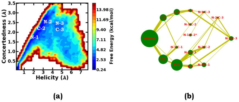
As mentioned earlier, the CHARMM22/CMAP energy potential biases the explicitly solvated Ala₁₀ to favor stepwise rather than commonly expected cooperative folding/unfolding pathways. Seeking to understand the cause, we define an order parameter, “concertedness”, to differentiate concerted and stepwise pathways. Specifically, concertedness is defined as the root mean square deviation, $\sqrt{\frac{{\sum }_{i=6}^{i=1}{\left(d_i-\overline{d}\right)}^2}{6}}$, in which d_i represents the distances of the α-helix hydrogen bonds and d̄ stands for the average value of these distances. It is noted that here, a lower concertedness value corresponds to a structure on a more concerted pathway and a higher value corresponds to a structure on a more stepwise pathway. As shown by the two-dimensional free energy profile with the helicity deviation and the concertedness as the collective variables, for any feasible transition between the helical state and the completely unfolded state, the pathway has to go through certain partially unfolded states with relatively high “concertedness” values, i.e. conformational intermediates characteristically representing stepwise transitions, such as the “N-3” or “C-3” state etc. This is due to the fact that these intermediates and their precursor intermediates, such as the “N-2” and “C-2” states, are relatively too stable.

To more comprehensively view the folding/unfolding pathways, based on the obtained samples, we constructed the thermodynamic network view of the free energy landscape (Figure 4b). In this network landscape, the area of each sphere is proportional to the population of the corresponding state and the width of each line is proportional to the number of the transitions between each pair of the states. The thermodynamic network reveals that there is no direct connection between the fully folded helical state and the completely unfolded (N-3/C-3) state. Interestingly, the completely unfolded (N-3/C-3) state is mainly connected with the “N-3” and “C-3” states; this suggests that for a short fragment with only three helical hydrogen bonds, the cooperative folding/unfolding transition is the dominant pathway. In order for the solvated Ala₁₀ peptide at either the “N-3” or “C-3” state to become fully folded, it has to follow a stepwise path, respectively going through the “N-2” state or “C-2” state, both of which can form local thermodynamic traps along the pathways. Moreover, our result shows that the C-terminus end is more stable than the N-terminus end and when the unfolding process is initiated from the N-terminus end, the system is most likely to be trapped at the over-stabilized N-2 and its accessory states, such as the N-2/C-1 and N-2/C-2 states, before proceeding to the complete unfolding state.

Figure 4.

The time-evolution of the Gaussian height in the Wang-Landau metadynamics simulation on model system 1.

The above analysis should provide insightful guidance for force field re-parameterization and refinement. For the fact that the gOST algorithm can enable detailed sampling of Ala₁₀ folding/unfolding processes, our method can serve as an essential part of a future routine procedure for protein energy function assessment.

Compensating Fluctuations of Solute-Solvent and Solute-Solute Interactions Drive Folding/Unfolding Transitions

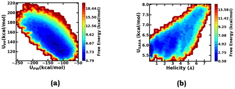
As discussed earlier, fluctuations of the essential solute-solute interaction energy (U_pp) are highly correlated with Ala₁₀ conformational changes (Figure 2d). In order to understand how solvent molecules influence helix-coil transitions, we constructed the two-dimensional free energy surface along both the essential solute-solvent interaction energy (U_PW) and U_pp (Figure 5a). Notably throughout the whole process, the essential solute-solvent and solute-solute interactions always intimately interplay. The solute-solvent and solute-solute interaction energies not only fluctuate in the opposite direction but also closely compensate each other. This observation suggests that solute conformational changes require synchronous solvent responses, which are featured by the compensating fluctuations of solute-solvent and solute-solution interactions; such observation further confirms the validity of the motivation underlying the gOST algorithm design. In addition to solute-solvent interactions, solvent-solvent interactions are also likely involved in solute conformational transitions. In gOST, a solvent-accessible-surface area (SASA) dependent term is introduced to accelerate near-solute solvent response fluctuations. As shown by Figure 5b, the SASA energy and the helicity deviation are also highly correlated; such close correspondence clearly demonstrates the importance of the SASA term in the gOST formulation.

Figure 5.

Calculated potential of mean forces on model system 2 based on three 600 ps simulations with different metadynamics setups. The line with triangles: calculated based on the metadynamics simulation employing the Wang-Landau recursion; the line with solid circles: calculated based on the metadynamics simulation using a low fixed Gaussian height (0.01 kcal/mol); the line with open circles: calculated based on the metadynamics simulation using a large fixed Gaussian height (0.1 kcal/mol).

Solvent Cooperative Transitions Play a Pivotal Role in Ala₁₀ Folding/Unfolding Processes

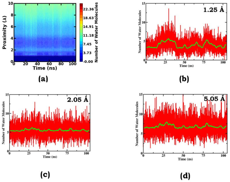
To understand how solvent structural changes couple with Ala₁₀ conformational transitions, we calculated the surface-proximity-dependent water number profile for each collected sample and monitored its time-dependent changes; here, the molecular surface definition and the surface-proximity-dependent water number calculation are based on the work of Willard & Chandler and each layer is defined as a shell with s thickness of 0.1 Å. As shown in Figure 6a, synchronous with solute structure changes, water structures undergo characteristic cooperative transitions, for instance in the layers that are 1.25 Å and 5.05 Å above the molecular surface. Taking a close look at the solvent layer that is 1.25 Å above the molecular surface (Figure 6b), we can easily tell that instead of slowly relaxing to equilibrium configurations after major solute conformational changes, water molecules undergo simultaneous configuration transitions. Such simultaneous transitions also occur in other distant layers, for instance the one that is 5.05 Å above the molecular surface (Figure 6d). Though with smaller amplitudes, the structural fluctuations of the distant layers, particularly from the local averaging view, display almost identical features as the fluctuations of the 1.25 Å layer. Even for the layers that undergo very small structural changes, for instance the one that is 2.05 Å above the molecular surface (Figure 6c), a similar transition pattern is also displayed. The above analysis reveals that near-solute solvent molecules are an integral part of the solute system; and water cooperative fluctuations occur simultaneously with and are essential to slow solute conformational transitions. Therefore in a sampling algorithm design, it is dangerous to empirically designate the solute region as the only “hot” area for active sampling treatment and the solvent region as the “cold” area to passively respond with the assumption that solvent structures always quickly fluctuate and relax.

Figure 6.

Fluctuation Behaviors of Common Energy Order Parameters

As discussed in the introduction, common “predictive” sampling methods, including TREM, HREM, ST, SS, and accelerated MD (aMD) etc. were formulated to enlarge the fluctuations of certain energy order parameters with the hope that promoted energy fluctuations can facilitate rare event barrier crossings. In practice, the effectiveness of a “predictive” sampling method strongly depends on how well fluctuations of the pre-chose energy order parameter correlate with progresses of molecular events. With less correlation, projected fluctuation enlargements on essential degrees of freedom are expected to be smaller and sampling efficiency is expected to be lower. As discussed above, fluctuations of the response order parameters in gOST significantly correlate with unfolding/folding transitions (Figure 2d and Figure 5a). This should naturally explain the effectiveness of the gOST method on the solvated Ala₁₀ model system.

Figure 7b shows that throughout the simulation, during which folding and unfolding events repetitively occur, the total potential energy does not display significant changes. As discussed earlier, during solute conformational transitions, distinct interaction components usually do not fluctuate in the same direction. Instead, on the solvated Ala₁₀ system, these essential interactions display a compensating fluctuation behavior; consequently, the fluctuation magnitude of the overall potential energy is very moderate. The two-dimensional free energy surface along the helicity deviation and the total potential energy reveals that there is no obvious correlation between conformational changes and total potential energy fluctuations. Due to its poor correlation with the conformational change, when the total potential energy is unselectively activated, only a small fraction of the fluctuation enlargement can be successfully projected onto the degrees of freedom essential to the conformational changes. Thus methods relying on total potential energy fluctuation promotion, such as TREM, ST, and the original aMD, are unlikely to be effective on Ala₁₀ folding/unfolding transitions.

Figure 7.

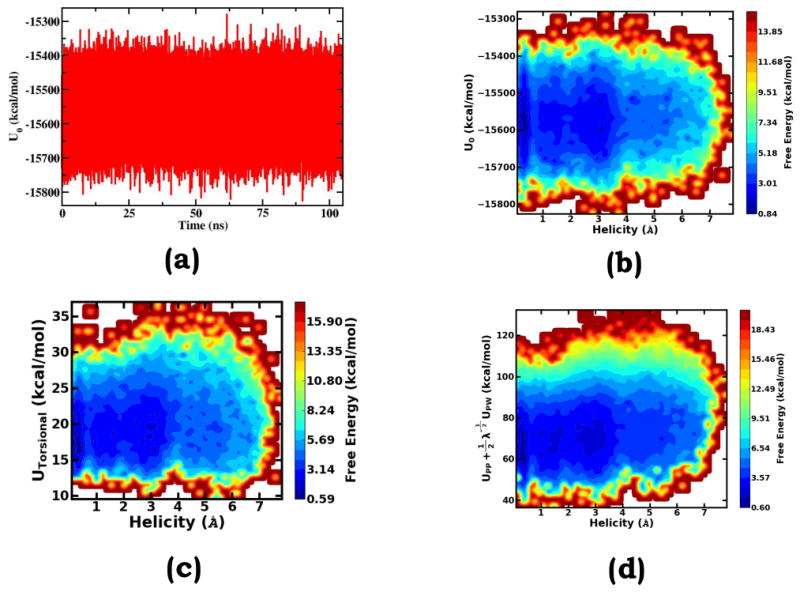
As an alternative, in some predictive sampling practices, the total solute torsional energy (corresponding to the sum of the total torsional energy and the total CMAP energy in this study) is employed as the sampling order parameter. Figure 7c shows that there is no obvious correlation between total torsional energy fluctuations and helix-coil transitions either. Therefore, we expect that enlarging the fluctuation of the total solution torsional energy alone is unlikely to enable effective sampling of the solvated Ala₁₀ peptide. It is worth noting that in our expanded Hamiltonian treatment, the total torsional energy is included in Uss(X_N). From the physical viewpoint, conformational transitions are governed by the fluctuations of both non-bond interaction energies and torsional energies. Together with the discussion in the previous subsection, we can tell that Ala₁₀ folding/unfolding transitions are mainly driven by solute-solute and solute-solvent electrostatic interaction fluctuations.

The HREM and ST methods are based on the general expanded Hamiltonian as described by Equation 1, which is employed as the basis of the perturbation treatment in this study. Specifically, we chose $\sqrt{\lambda }$ for SE(λ), which in the HREM context is also called the solute tempering II treatment. To assess methods based on Equation 1, we evaluate which is featured with usually correspond to certain enduring configurations, and once a while undergoes sharp transitions between one and another. Notably such cooperative transitions usually indicate the occurrence of conformational events. As commonly known, α-helix is the most stable order form of undergoes several critical cooperative fluctuation transitions.

The gOST algorithm was implemented in our customized version of the CHARMM program^28,29. In this study, we selected all the intra-peptide torsional (including the CMAP) and electrostatic energy terms into U_ss(X_N), which is denoted as U_PW in the section of Results and and all the electrostatic interactions between the peptide and the solvent environment (including both water molecules and ions) into U_se(X_N). For SE(λ), we picked $\sqrt{\lambda }$ for no particular reason other than that it is a commonly used function form for HREM based simulations. For U_sasa(X_N), we used a surface-accessible-surface-area dependent functional form in the CHARMM program. We collected temperature-dependent water surface tension changes γ(T_m) and set SASA(λ) as a B-spline function connecting the points based on

Table 1. The collective variable definitions and descriptions.

CVs	Definitions	Descriptions
θ1	OE1 – HE1	To model the bond breaking/forming events responsible for the proton transfer
θ2	Ob – HE1
θ3	OE1 – Ob	To describe geometrical changes coupled with the proton transfer
θ4	OE2 – HE1
θ5	Ob – C	To model the bond breaking/forming events for the SN2 substitution
θ6	OAc – C
θ7	C4 – C	To describe bond orientation changes coupled with the SN2 substitution
θ8	CAc – C

References

- 1.Jorgensen WL. Acc Chem Res. 1989;22:184. [Google Scholar]; Raugei S, Kim D, Klein ML. Quant Struc Act Relat. 1989;21:149. [Google Scholar]; Benkovic SJ, Hammes-Schiffer S. Science. 1989;301:1196. doi: 10.1126/science.1085515. [DOI] [PubMed] [Google Scholar]; Garcia-Viloca M, Gao J, Karplus M. Science. 1989;303:186. doi: 10.1126/science.1088172. [DOI] [PubMed] [Google Scholar]; Gao JL, Ma S, Major DT, Nam K, Pu JZ, Truhlar DG. Chem Rev. 2006;106:3188. doi: 10.1021/cr050293k. [DOI] [PMC free article] [PubMed] [Google Scholar]
- 2.Bahar I. Rev Chem Eng. 1999;15:319. [Google Scholar]; Gao JL, Byun KL, Kluger R. Top Curr Chem. 1989;238:113. [Google Scholar]; Hummer G, Szabo A. Acc Chem Res. 2005;38:504. doi: 10.1021/ar040148d. [DOI] [PubMed] [Google Scholar]; Tama F, Brooks CL. Ann Rev Biophys Biomol Struc. 2006;35:115. doi: 10.1146/annurev.biophys.35.040405.102010. [DOI] [PubMed] [Google Scholar]
- 3.Tobias DJ, Tu KC, Klein ML. Curr Opin Coll Inter Sci. 1989;2:15. [Google Scholar]; Muthukumar M. Adv Poly Sci. 2005;191:241. [Google Scholar]
- 4.Gilson MK, Given JA, Bush BL, McCammon JA. Biophys J. 1989;72:1047. doi: 10.1016/S0006-3495(97)78756-3. [DOI] [PMC free article] [PubMed] [Google Scholar]; Kollman PA, et al. Acc Chem Res. 1989;33:889. doi: 10.1021/ar000033j. [DOI] [PubMed] [Google Scholar]; Simonson T, Archontis G, Karplus M. Acc Chem Res. 1989;35:430. doi: 10.1021/ar010030m. [DOI] [PubMed] [Google Scholar]; Jorgensen WL. Science. 2004;303:1813. doi: 10.1126/science.1096361. [DOI] [PubMed] [Google Scholar]; Gilson MK, Zhou HX. Ann Rev Biophys Biomol Struc. 1989;36:21. doi: 10.1146/annurev.biophys.36.040306.132550. [DOI] [PubMed] [Google Scholar]; Peters MB, Raha K, Merz KM. Curr Opin Drug Disc Dev. 2006;9:370. [PubMed] [Google Scholar]
- 5.Patey GN, Valleau JP. J Chem Phys. 1989;63:2334. [Google Scholar]; Kumar S, Bouzida D, Swendsen RH, Kollman PA, Rosenberg JM. J Comp Chem. 1992;13:1011. [Google Scholar]
- 6.Mezei M. J Comp Phys. 1987;68:237. [Google Scholar]; Bartels C, Karplus M. J Comp Chem. 1997;18:1450. [Google Scholar]
- 7.Hamelberg D, Mongan J, McCammon JA. J Chem Phys. 2004;120:11919. doi: 10.1063/1.1755656. [DOI] [PubMed] [Google Scholar]
- 8.Rahman JA, Tully JC. J Chem Phys. 2002;116:8750. [Google Scholar]
- 9.Voter AF. Phys Rev Lett. 1997;78:3908. [Google Scholar]
- 10.Grubmuller H. Phys Rev E. 1995;52:2893. doi: 10.1103/physreve.52.2893. [DOI] [PubMed] [Google Scholar]
- 11.Laio A, Parrinello M. Proc Natl Acad Sci USA. 2002;99:12562. doi: 10.1073/pnas.202427399. [DOI] [PMC free article] [PubMed] [Google Scholar]
- 12.Ensing B, De Vivo M, Liu Z, Moore P, Klein ML. Acc Chem Res. 2006;39:73. doi: 10.1021/ar040198i. [DOI] [PubMed] [Google Scholar]
- 13.Iannuzzi M, Laio A, Parrinello M. Phys Rev Lett. 2003;90:238302. doi: 10.1103/PhysRevLett.90.238302. [DOI] [PubMed] [Google Scholar]; Iannuzzi M, Laio A, Parrinello M. Phys Rev Lett. 1989;92:170601. doi: 10.1103/PhysRevLett.92.170601. [DOI] [PubMed] [Google Scholar]; Ensing B, Laio A, Parrinello M, Klein ML. J Phys Chem B. 2005;109:6676. doi: 10.1021/jp045571i. [DOI] [PubMed] [Google Scholar]
- 14.Laio A, Rodriguez-Fortea A, Luigi Gervasio F, Ceccarelli M, Parrinello M. J Phys Chem B. 2005;109:6714. doi: 10.1021/jp045424k. [DOI] [PubMed] [Google Scholar]
- 15.Wang FG, Landau DP. Phys Rev Lett. 2001;86:2050. doi: 10.1103/PhysRevLett.86.2050. [DOI] [PubMed] [Google Scholar]
- 16.Li H, Fajer M, Yang W. J Chem Phys. 2007;126:24106. doi: 10.1063/1.2424700. [DOI] [PubMed] [Google Scholar]
- 17.Warshel A, Levitt M. J Mol Biol. 1989;103:227. doi: 10.1016/0022-2836(76)90311-9. [DOI] [PubMed] [Google Scholar]; Madura JD, Jorgensen WL. J Am Chem Soc. 1989;108:2517. [Google Scholar]; Field MJ, Bash PA, Karplus M. J Comp Chem. 1989;11:700. [Google Scholar]; Gao JL. Acc Chem Res. 1989;29:298. [Google Scholar]; Monard G, Merz KM. Acc Chem Res. 1999;32:904. [Google Scholar]
- 18.Berg BA. Markov Chain Monte Carlo Simulations and Their Statistical Analysis. World Scientific; Singapore: 2004. [Google Scholar]
- 19.Brooks BR, Bruccoleri RE, Olafson BD, States DJ, Swaminathan S, Karplus M. J Comp Chem. 1983;4:187. [Google Scholar]
- 20.MacKerell AD, et al. CHARMM parameter Group. J Phys Chem B. 1998;102:3586. [Google Scholar]
- 21.Matthews RG, Goulding CW. Curr Opin Chem Biol. 1997;1:332. doi: 10.1016/s1367-5931(97)80070-1. [DOI] [PubMed] [Google Scholar]
- 22.Cui Q, Elstner M, Kaxiras E, Frauenheim T, Karplus M. J Phys Chem B. 2001;105:569. [Google Scholar]
- 23.Jorgensen WL, Chandrasekhar J, Madura JD, Impey RW, Klein ML. J Chem Phys. 1983;79:926. [Google Scholar]
- 24.Pesonen J, Halonen L. J Chem Phys. 2002;116:1825. [Google Scholar]
- 25.Frederick JH, Woywod C. J Chem Phys. 1999;111:7255. [Google Scholar]
- 26.Chapuisat X, Iung C. Phys Rev A. 1992;45:6217. doi: 10.1103/physreva.45.6217. [DOI] [PubMed] [Google Scholar]