Establishment of Biological Reference Intervals and Reference Curve for Urea by Exploratory Parametric and Non-Parametric Quantile Regression Models

Abstract

Background: The validity of the entire renal function tests as a diagnostic tool depends substantially on the Biological Reference Interval (BRI) of urea. Establishment of BRI of urea is difficult partly because exclusion criteria for selection of reference data are quite rigid and partly due to the compartmentalization considerations regarding age and sex of the reference individuals. Moreover, construction of Biological Reference Curve (BRC) of urea is imperative to highlight the partitioning requirements.

Materials and Methods: This a priori study examines the data collected by measuring serum urea of 3202 age and sex matched individuals, aged between 1 and 80 years, by a kinetic UV Urease/GLDH method on a Roche Cobas 6000 auto-analyzer.

Results: Mann-Whitney U test of the reference data confirmed the partitioning requirement by both age and sex. Further statistical analysis revealed the incompatibility of the data for a proposed parametric model. Hence the data was non-parametrically analysed. BRI was found to be identical for both sexes till the 2^nd decade, and the BRI for males increased progressively 6^th decade onwards. Four non-parametric models were postulated for construction of BRC: Gaussian kernel, double kernel, local mean and local constant, of which the last one generated the best-fitting curves.

Conclusion: Clinical decision making should become easier and diagnostic implications of renal function tests should become more meaningful if this BRI is followed and the BRC is used as a desktop tool in conjunction with similar data for serum creatinine.

INTRODUCTION

One of the three most commonly prescribed blood tests by physicians, Urea is the major end product of protein nitrogen metabolism^1,2. It is synthesized by the Urea Cycle in the liver from ammonia which is produced by amino acid deamination. Most of the urea thus produced is eliminated by glomerular filtration, with 40 – 60% diffusing back into the blood, irrespective of the proximal tubular flow rate. Rediffusion in the distal tubule depends on the urinary flow and is regulated by Anti-diuretic Hormone. During diuresis, there is minimal rediffusion and blood urea levels are low, whereas during anti-diuresis, the opposite happens. Thus blood urea levels depend on urea synthesis rate, renal perfusion and glomerular filtration rate (GFR). When used in conjunction with serum creatinine, determination of serum urea can aid in the differential diagnosis of three types of azotaemia: prerenal, renal and postrenal.

Biological reference interval (BRI) of urea is a critical component, and the validity of the entire renal function tests as a diagnostic tool depends on it. The BRI should provide an acceptable degree of confidence for the decision-making process, which includes a consideration of the significant factors and variables introduced by the specific individual’s reference sample or by the analytical process itself³. Establishment of BRI for urea is cumbersome⁴ as one has to exclude both hepatic and renal disorders, two of the commonest community afflictions, while selecting reference individuals. Secondly, protein metabolism differs in the two sexes, thereby accounting for the possibility of sex-wise segregation of reference values. Thirdly, protein anabolism takes the upper hand in children and adolescents vis-à-vis the elderly individuals who predominantly catabolize proteins, compounded with the fact that renal function decreases with age; this adds a further dimension of age-wise compartmentalization of reference values. As a result, most of the literature supplied with the reagents refers to a broad classification of reference values. For example, the reagent kit used in this study refers to the expected values of <50 mg/dL for individuals <65 years and <71 mg/dL for indiviuals >65 years. One is tempted to ask how often would you find a 10 year old healthy child with serum urea as high as, say, 45 mg/dL (which is normal as per the kit insert)!

This article objectively describes the establishment of BRI for urea measured on an urban Indian ambulatory population by a kinetic UV Urease/GLDH method using dedicated reagents of Cobas 6000 auto-analyzer on the basis of guidelines set by the CLSI C28-A3 document⁵. Inclusion of a graphical representation in the form of a Biological Reference Curve (BRC) adds interpretive value to the information, especially when partitioning of reference data is expected.

MATERIALS AND METHODS

This a priori non-interventional, cross-sectional unicentric observation was undertaken during the calendar year of 2012, in the Department of Biochemistry, Drs. Tribedi & Roy Diagnostic Laboratory Pvt. Ltd., Kolkata, India on issuance of a statutory Ethical Committee approval.

Subjects: The subjects were selected on the basis of a direct sampling technique, as practised in any a priori procedure. Age and sex matched individuals were selected according to pre-determined inclusion criteria (vide Table 1). A total number of 3202 subjects (Males = 1596, Females = 1606), aged between 1 and 80 years were selected for the study, in each case, after the execution of an informed consent.

Table 1.

Inclusion and exclusion criteria exercised while sampling

Inclusion Criteria: Age between 1 and 80 years. Body Mass Index (BMI) between 18.5 and 30 kg/m2. 10 to 14 hours of overnight fasting. Sample collection between 8:00 AM and 12:00 noon.

Exclusion Criteria: Past or present history of renal and hepatic disorders. Deranged Liver Function Tests and/or serum creatinine. Acute illness, under current or long-term medication of any sort. Grossly haemolysed, lipaemic or icteric samples.

Samples: Venous blood samples were collected after allowing 10 to 15 minutes of rest in an office environment, observing standard aseptic procedures, within 30 seconds of tying tourniquet and transferred to standard gel separator tubes^6,7. All samples were tested on the same day of collection.

Methods: The samples were measured on a Cobas 6000 (Roche Diagnostics GmbH) platform using dedicated Urease/GLDH reagents8. It is a kinetic method where urea is hydrolysed by urease to form ammonia and carbonate:

In the second reaction, 2-oxoglutarate reacts with ammonium in the presence of glutamate dehydrogenase (GLDH) and the coenzyme NADH to produce L-glutamate. In this reaction two moles of NADH are oxidized to NAD+ for each mole of urea hydrolysed:

The rate of decrease of NADH concentration is directly proportional to the urea concentration in the specimen and is measured photometrically at 340 nm.

Performance specifications claimed by the instrument’s manufacturer pertaining to the urea method⁹ are listed in Table 2.

Table 2.

Performance specifications of Urea method on Cobas 6000

Analytical Sensitivity (value lying 3 SD above the zero calibrator in a repeatability study, n=21): 3 mg/dL. Analytical Measurement Range: 3 – 240 mg/dL (or up to 720 mg/dL for 3 fold diluted samples). Precision: Within run – 0.9 to 1.0 %CV, Across-run – 1.1 to 1.3 %CV. Accuracy (as per evaluations through one year on a commercial 3rd party EQA programme): 1.4 to 3.6 %. Interferences: No significant interferences were observed by haemolysis up to 1 g/dL of Hb, lipaemia up to 1500 mg/dL of Intralipid, icterus up to 60 mg/dL of bilirubin. Ammonium ions cause false elevation of results. Waldenstrom’s macroglobulinaemia (IgM) may cause unreliable results.

Certain components of the performance indicators e.g. analytical measurement range, precision and accuracy verified by this laboratory matches the manufacturer’s claims. Method calibrations were performed routinely once every week, on changes of lots of reagents and calibrators and as corrective measures for QC outliers. Two levels of commercial control materials were run on every working day (Level 1 target value = 40 mg/dL, range = 35 to 45 mg/dL; Level 2 target value = 140 mg/dL, range = 130 to 150 mg/dL) and standard Westgard warning (1_2s,4_1s) and run rejection (1_3s,2_2s,R_4s,10_x) rules were applied^10,11. The study was spaced out into a whole calendar year deliberately to even out the variations brought in by changes in lots of reagents, calibrators and in instrument calibrations. In particular, two lots of calibrators and five lots of reagents were used during this period.

Statistical Analyses: The data thus obtained were first analysed to establish the partitioning requirements of two covariates, namely age and sex. Then the data were subjected to tests for determining its suitability for parametric treatment. Finally non-parametric methods were applied for computation of BRI and construction of BRC.

RESULTS & DISCUSSION

Partitioning Requirement^12,13: To verify whether the distribution of the serum urea values is influenced by age of the subjects, the weighted residuals of the urea values were plotted as a function of age (vide Figure 1), where weighted residual (𢀘), is defined as 𢀘 = (yi – m)/σ, where yi is the individual urea value, m is the population mean and o is the population SD14. If the weighted residuals are arranged in a band of constant width around the zero line, it may be assumed that the urea values do not change significantly with age. As is evident from Figure 1, a constant bandwidth was not maintained, there was significant dispersion both above and below the zero line, and most importantly there was significant spiking above and below the zero line corresponding to the change of decades, e.g. 11 years, 21 years and so on. This signified that not only age-wise partitioning of the data was required but also a decade-wise partitioning would be appropriate. To determine if the sex of the subjects influenced the distribution of data, the data was segregated into two groups (Male = 1596, Female = 1606) and the non-parametric Mann-Whitney U test¹⁵ was run to compare the two groups, which returned a Z-statistic of 12.157 with a P-value of <0.0001, implying that the two groups were significantly different (P<0.05). Thus, sex-specific partitioning was also required for this particular data set.

Figure 1.

Weighted residuals [𢀘 = (yi – m)/σ] of serum urea values plotted as a function of age. The data points are not evenly distributed in a constant width above and below the 𢀘 = 0 line, additionally there are significant spikes with the change of decades, thereby implying that age distribution of urea values are not homoscedastic, and partitioning by age is necessary.

Fitness for Parametric Estimation: As it was determined that sex-specific partitioning was imperative, henceforth, the data would be segregated into two (Males & Females) and each group would be subjected to tests determining its fitness for parametric estimation. For parametric methods to be applicable, the following conditions must be met¹⁶:

1. For each value of covariate (e.g. age) the distribution of data, either raw or transformed, is Gaussian.

2. The population mean of the analyte, here urea, is a linear function of age, i.e.,

   m = a + b x Age Eqn. 1

3. The dispersion of urea values (i.e. standard deviation σ) does not vary with age; in other words, the data is homoscedastic.

When for each value of the covariate the data distribution is not Gaussian, a data transformation can be used to “normalize” the distribution. Several families of transformations are used by statisticians among which, the Box-Cox transformation is likely the most famous^17,18. The Box-Cox transformation with parameter λ is given by (y^λ – 1)/λ. When λ = 1, this transformation is linear implying that there is no need to transform the data to normalize their distribution. When λ = 0, this transformation becomes the natural logarithm ln(y). This suggests that taking the natural logarithm of the data should normalize their distribution. Analysis of the current data returned a λ values of 0.498 and 0.801 for males and females respectively, which were different from 1 (P<0.001), hence Box-Cox transformation was required, and were different from 0 (again, P<0.001), hence logarithmic transformation would not be helpful.

The data was statistically analysed to determine the values of the functions a and b in Eqn. 1. The values were obtained thus: Males: a = 6.746, b = 0.066; Females: a = 12.637, b = 0.142. These functions, along with the corresponding λ values, when put into Eqn. 1, generate the working equations for BRI computation thus:

Males: (Urea^0.498 – 1)/0.498 = 6.746 + 0.066 x Age Eqn. 2

Females: (Urea^0.801 – 1)/0.801 = 12.637 + 0.142 x Age Eqn. 3

Thereby, a parametric model was established for the urea data and Eqns. 2 & 3 can be utilized for construction of BRCs, but it was still necessary to determine whether this model appropriately describes the data. This can be suitably evaluated by inspecting a graph whereby the Box-Cox transformed data is plotted as a function of the best fit values^19,20. The fitted values are obtained by back-transformation thus:

Males: Urea = {1 + 0.498 x (6.746 + 0.066 x Age)}^1/0.498 Eqn. 4

Females: Urea = {1 + 0.801 x (12.637 + 0.142 x Age)}^1/0.801 Eqn. 5

This is depicted in Figure 2, where Box-Cox transformed data were plotted on y-axis and fitted values, as calculated by Eqns. 4 & 5, on x-axis. The magnitude of dispersion on the y-axis gives information on the actual dispersion of the data. The magnitude of dispersion on the x-axis gives information on what the model explains. As is evident from the figure, for males, the Box-Cox transformed data span 8 – 70 mg/dL, whereas the fitted values span 20 – 50 mg/dL; for females, the corresponding figures were 8 – 57 mg/dL and 20 – 42 mg/dL respectively. In other words, the proposed model explains only 58.8% and 49.7% of the male and female data respectively. This is evidence strong enough to reject the parametric model and move on to non-parametric models to obtain the objective of this study.

Figure 2.

Parametric model validation plot for (A) males and (B) females. Box-Cox transformed values of serum urea are plotted as a function of back-transformed fitted values. The diagonal through the origin is the first bisector line. Kindly refer to the text for details.

Proposed Non-parametric Models: As guided by the Age vs. Weighted Residuals plot, decade-wise BRIs of Serum Urea for Males and Females were computed by non-parametric method (vide Table 3). Ninety percent confidence intervals for lower and upper reference limits were calculated using a non-parametric bootstrap method²¹. It may be noted that BRIs for both males and females remain the same till the 2^nd decade, whereas values for males increase significantly from the 6^th decade onwards.

Table 3.

Results of a Non-parametric estimation of Biological Reference Interval of Serum Urea (in mg/dL)

Age, in yrs.	Males (N = 1596)					Females (N = 1606)
	N	Lower Limit	90% Cl(L)*	Upper Limit	90% Cl(U)†	N	Lower Limit	90% Cl(L)*	Upper Limit	90% Cl(U)†
1 – 10	197	10	10 – 11	25	24 – 25	197	10	10 – 11	25	24 – 25
11 – 20	203	14	14 – 15	34	34 – 35	201	14	14 – 15	34	34 – 35
21 – 30	207	19	19 – 20	40	39 – 40	209	19	19 – 20	40	39 – 40
31 – 40	192	24	23 – 25	45	44 – 45	189	24	23 – 25	40	39 – 40
41 – 50	213	25	24 – 25	48	48 – 49	219	24	23 – 25	45	44 – 45
51 – 60	209	25	24 – 25	53	53 – 54	205	25	24 – 25	48	48 – 49
61 – 70	189	30	29 – 30	59	59 – 60	192	25	24 – 25	48	48 – 49
71 – 80	186	34	34 – 35	68	67 – 68	194	30	29 – 30	54	53 – 54

Note: * 90% Confidence Interval of Lower Reference Limit

† 90% Confidence Interval of Upper Reference Limit

Reference curves were constructed using non-parametric quantile regression technique^22,23, where the relation between the independent variable (predictor) e.g. Age, and the independent variable (response) e.g. Urea value is not determined by a predetermined equation but according to the information derived from the data itself. Each reference curve consists of three lines corresponding to 2.5 percentile, 50 percentile and 97.5 percentile respectively. Each line represents the best fitted series of points but not a pre-determined equation^24,25. Four models of non-parametric regression were used: in the 1^st model Gaussian kernels²⁶for Age were used to estimate the dispersion of Urea values; in the 2^nd model, two kernels were used: a Gaussian kernel for the x-axis and an uniform kernel for the y-axis; in the 3^rd model local constant theory was applied where the means for sets of data points are joined to form the regression line; in the 4^th model local linear theory was applied where the best fitting lines for each point are joined together to form the regression line. Figure 3 represents these findings for male reference data and Figure 4 depicts the same for female reference data. Choice for the candidate reference curve mainly depends on the smoothness of the regression lines thus derived^27,28. In this case, the local linear model (Figure 3D, Figure 4D) produces the desired level of smoothness and thus may be chosen as the candidate Biological Reference Curve for Serum Urea by Urease/GLDH method.

Figure 3.

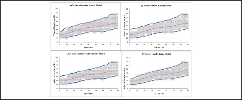
Non-Parametric Regression models applied on the urea data for males to construct a Biological Reference Curve: (A) Gaussian kernel model, (B) Double kernel model, (C) Local Constant (Mean) model and (C) Local Linear model. The lower and upper lines represent the 2.5 and 97.5 percentile limits respectively. The middle line represents the 50th percentile level.

Figure 4.

Non-Parametric Regression models applied on the urea data for females to construct a Biological Reference Curve: (A) Gaussian kernel model, (B) Double kernel model, (C) Local Constant (Mean) model and (C) Local Linear model. The lower and upper lines represent the 2.5 and 97.5 percentile limits respectively. The middle line represents the 50th percentile level.

CONCLUSION

BRI established and BRC constructed in this exercise can be used as a very powerful diagnostic tool. When used in conjunction with a similar data for serum creatinine, this model can make clinical decision making quite a cake-walk. One can easily diagnose or exclude azotaemia as a rule of the thumb, just by inspecting the BRC. Furthermore, the mathematical models proposed in this study are valid for any other analyte and can be applied in any diagnostic specialty.

References

- 1.Thomas L. Urea and blood urea nitrogen (BUN). Thomas L, ed. Clinical laboratory diagnostics. Use and assessment of clinical laboratory results. Frankfurt/Main: TH-Books Verlagsgesellschaft, 1998; 374-377. [Google Scholar]
- 2.Newman DJ, Price CP. Renal function and nitrogen metabolites. Burtis CA, Ashwood ER, eds. Teitz textbook of clinical chemistry, 3rd ed. Philadelphia: WB Saunders Company, 1999; 1239-1241. [Google Scholar]
- 3.Solberg HE. Establishment and use of reference values. Burtis CA, Ashwood ER, eds. Teitz textbook of clinical chemistry, 3rd ed. Philadelphia: WB Saunders Company, 1999. [Google Scholar]
- 4.Heil W, Koberstein R, Zawta B. Reference ranges for adults and children. Pre-analytical considerations, 8th ed. Roche Diagnostics, 2004. [Google Scholar]
- 5.Clinical and Laboratory Standards Institute. Defining, establishing and verifying reference intervals in the clinical laboratory: approved guideline, 3rd ed. CLSI document C28-A3: Wayne PA, Clinical and Laboratory Standards Institute, 2008; 28(30): pp 61. [Google Scholar]
- 6.World Health Organization. Laboratory Biosafety Manual. 3rd ed. Geneva: World Health Organization; 2004. [Google Scholar]
- 7.Clinical and Laboratory Standards Institute. Protection of Laboratory Workers from Occupationally Acquired Infections: Approved Guidelines-Third Edition. CLSI Document M29-A3. Wayne PA: Clinical and Laboratory Standards Institute; 2005. [Google Scholar]
- 8.Sampson EJ, Baired MA, Burtis CA, Smith EM, Witte DL, Bayse DD. A coupled – enzyme equilibrium method for measuring urea in serum: Optimization and evaluation of the AACC study group on urea candidate reference method. Clin Chem 1980; 26:816-826. [PubMed] [Google Scholar]
- 9.Urea Reagent Kit Literature for Cobas c501, Roche Diagnostics. Mannheim:2006. [Google Scholar]
- 10.Westgard JO, Barry PL, Hunt MR. A multi-rule Shewhart chart for quality control in clinical chemistry. Clin Chem 1981; 27:493–501. [PubMed] [Google Scholar]
- 11.Westgard JO, Groth T, Aronsson T, Falk H, de Verdier CH. Performance characteristics of rules for internal quality control: probabilities for false rejection and error detection. Clin Chem 1977; 23:1857–1887. [PubMed] [Google Scholar]
- 12.Lahti A. Partitioning biochemical reference data into subgroups: comparison of existing methods. Clin Chem Lab Med 2004; 42:725–733. [DOI] [PubMed] [Google Scholar]
- 13.Harris E, Boyd JC. On dividing reference data into subgroups to produce separate reference ranges. Clin Chem 1990; 36:265–270. [PubMed] [Google Scholar]
- 14.Grambsch P, Therneau T. Proportional hazards test and diagnostics based on weighted residuals. Biometrika, 1994; 81:515-526. [Google Scholar]
- 15.Mann HB, Whitney DR. On a Test of Whether one of Two Random Variables is Stochastically Larger than the Other. Annals of Mathematical Statistics 1947; 18(1):50–60. [Google Scholar]
- 16.Horn PS. A biweight prediction interval for random samples. J Am Stat Assoc 1988; 83:249-256. [Google Scholar]
- 17.Box GEP, Cox DR. An analysis of transformations. J.R. Stat. Soc. B 1964; 26:211-252. [Google Scholar]
- 18.Draper NR, Cox DR. On distributions and their transformation to normality 1969; J. R. Stat. Soc. B 31:472-476. [Google Scholar]
- 19.Hurvich CM, Tsai CL. The impact of model selection on inference in linear regression. American Statistician, 1990; 44:214-217. [Google Scholar]
- 20.Davidian M, Giltinan DM. Nonlinear Models for Repeated Measurement Data, New York: Chapman and Hall, 1995. [Google Scholar]
- 21.Efron B, Tibshirani R. An Introduction to the Bootstrap. Chapman and Hall, New York, 1993. [Google Scholar]
- 22.Gannoun A, Girard S, Guinot C, Saracco J. Reference curves based on nonparametric quantile regression. Stat. in Med., 2002; 21, 3119-3135. [DOI] [PubMed] [Google Scholar]
- 23.Gannoun A, Girard S, Guinot C, Saracco J. Sliced inverse regression in reference curves estimation. Computational Statistics and Data Analysis, 2004; 46(1), 103-122. [Google Scholar]
- 24.Samanta T. Non-parametric estimation of conditional quantiles. Statistics and Probability Letters, 1989; 407–412. [Google Scholar]
- 25.Chaudhuri P. Global nonparametric estimation of conditional quantile functions and their derivative. Journal of Multivariate Analysis, 1991; 246–269. [Google Scholar]
- 26.Smola AJ, Sch¨olkopf B. On a kernel-based method for pattern recognition, regression, approximation and operator inversion. Algorithmica, 1998; 22:211–231. [Google Scholar]
- 27.Bosch RJ, Ye Y, Woodworth GG. A convergent algorithm for quantile regression with smoothing splines. Computational Statistics and Data Analysis, 1995; 19:613–630. [Google Scholar]
- 28.Bowman AW, Azzalini A. Applied smoothing techniques for data analysis. Calarendon Press, Oxford: 1997. [Google Scholar]