Deep learning for digital pathology image analysis: A comprehensive tutorial with selected use cases

Abstract

Background:

Deep learning (DL) is a representation learning approach ideally suited for image analysis challenges in digital pathology (DP). The variety of image analysis tasks in the context of DP includes detection and counting (e.g., mitotic events), segmentation (e.g., nuclei), and tissue classification (e.g., cancerous vs. non-cancerous). Unfortunately, issues with slide preparation, variations in staining and scanning across sites, and vendor platforms, as well as biological variance, such as the presentation of different grades of disease, make these image analysis tasks particularly challenging. Traditional approaches, wherein domain-specific cues are manually identified and developed into task-specific “handcrafted” features, can require extensive tuning to accommodate these variances. However, DL takes a more domain agnostic approach combining both feature discovery and implementation to maximally discriminate between the classes of interest. While DL approaches have performed well in a few DP related image analysis tasks, such as detection and tissue classification, the currently available open source tools and tutorials do not provide guidance on challenges such as (a) selecting appropriate magnification, (b) managing errors in annotations in the training (or learning) dataset, and (c) identifying a suitable training set containing information rich exemplars. These foundational concepts, which are needed to successfully translate the DL paradigm to DP tasks, are non-trivial for (i) DL experts with minimal digital histology experience, and (ii) DP and image processing experts with minimal DL experience, to derive on their own, thus meriting a dedicated tutorial.

Aims:

This paper investigates these concepts through seven unique DP tasks as use cases to elucidate techniques needed to produce comparable, and in many cases, superior to results from the state-of-the-art hand-crafted feature-based classification approaches.

Results:

Specifically, in this tutorial on DL for DP image analysis, we show how an open source framework (Caffe), with a singular network architecture, can be used to address: (a) nuclei segmentation (F-score of 0.83 across 12,000 nuclei), (b) epithelium segmentation (F-score of 0.84 across 1735 regions), (c) tubule segmentation (F-score of 0.83 from 795 tubules), (d) lymphocyte detection (F-score of 0.90 across 3064 lymphocytes), (e) mitosis detection (F-score of 0.53 across 550 mitotic events), (f) invasive ductal carcinoma detection (F-score of 0.7648 on 50 k testing patches), and (g) lymphoma classification (classification accuracy of 0.97 across 374 images).

Conclusion:

This paper represents the largest comprehensive study of DL approaches in DP to date, with over 1200 DP images used during evaluation. The supplemental online material that accompanies this paper consists of step-by-step instructions for the usage of the supplied source code, trained models, and input data.

INTRODUCTION

Digital pathology (DP) is the process by which histology slides are digitized to produce high-resolution images. DP is becoming increasingly common due to the growing availability of whole slide digital scanners.[1] These digitized slides afford the possibility of applying image analysis techniques to DP for applications in detection, segmentation, and classification. Already algorithmic approaches have shown to be beneficial in many contexts as they have the capacity to not only significantly reduce the laborious and tedious nature of providing accurate quantifications (e.g., tumor extent, nuclei counts), but to act as a second reader helping to reduce inter-reader variability among pathologists.[2,3]

A number of image analysis tasks in DP involve some sort of quantification (e.g., cell or mitosis counting) or tissue grading (classification). As shown in Figure 1, these tasks invariably require identification of histologic primitives (e.g., nuclei, mitosis, tubules, epithelium, etc.). For example, while the spatial arrangement of nuclei in oropharyngeal[4] and breast cancers[5] has been correlated with outcome, these approaches still initially requiring deep annotations (i.e., various entities identified at different scales) to extract features from. As a result, there is a strong need to develop efficient and robust algorithms for analysis of DP images.

Figure 1.

The flowchart shows a typical workflow for digital pathology research. Histologic primitives (e.g. nuclei, lymphocytes, mitosis, etc.,) are identified, after which biologically relevant features are extracted for subsequent use in higher order research directives. Typically, the tasks in the red box are undertaken by the development and upkeep of individual task specific approaches. The premise of this tutorial is that these tasks can be performed by a single generic deep learning approach, which can be easily maintained and extended upon

While there have been a number of papers in the area of computational image analysis of DP images for the purposes of object detection and quantification in the last few years, there appear to be two main drawbacks to existing approaches. First, the development of task specific approaches tends to require long research and development cycles. For example, to develop a nuclei segmentation algorithm, one must first understand all of the possible variances in morphology, texture, and color appearances. Subsequently, an algorithmic scheme needs to be developed which can account for as many of these variances as possible while not being too general as to result in false positive results or too narrow as to result in false negative errors. This process can become quite unwieldy as it is often infeasible to view all of the outlier cases a priori, and thus an extensive iterative trial and error approach needs to be undertaken. Unfortunately, once a suitable set of operating parameters is found for a specific dataset, it is unlikely to directly translate to a second independent dataset, typically requiring additional parameter tweaking and tuning. This leads to the second drawback with existing approaches; the implicit knowledge of how to find or adjust optimal parameters often resides solely with the developers of the algorithms and thus are not intuitively understood by external parties. In addition, note the process above describes only a single task, in the case where a DP suite is created, consisting of a single approach for each desired task (e.g., segmentation of nuclei, detection of mitosis, etc.), there is a multiplicative burden of both steep learning curves of the nuances of each algorithm as well as the general maintenance and upkeep of multiple software projects. Together, these create a strong hindrance for researchers to leverage or extend the available technology to investigate their clinical hypothesis.

Deep learning (DL) is an example of the machine learning paradigm of feature learning; wherein DL iteratively improves upon learned representations of the underlying data with the goal of maximally attaining class separability. This is to say that every DL network begins with the same assumption of random initialization, and for each iteration, data are propagated through the network to compute its respective output. This output is compared to the desired output (e.g., determining if a pixel in question belongs to a nucleus or not), and an error is computed per parameter so that it can be adjusted to better dichotomize that training sample into the correct class. We note that there are no preexisting assumptions about the particular task or dataset, in the form of encoded domain-specific insights or properties, which guide the creation of the learned representation. The DL approach involves deriving a suitable feature space solely from the data itself. This is a critical attribute of the DL family of methods, as learning from training exemplars allows for a pathway to generalization of the learned model to other independent test sets. Once the DL network has been trained with an adequately powered training set, it is usually able to generalize well to unseen situations, obviating the need of manually engineering features.

DL is thus uniquely suited to analyze big data repositories (e.g., TCGA, which currently comprises over 1 petabyte worth of digital tissue slide images), as it is ideally suited to learn in an implicit fashion the diversity of image patterns embedded within large datasets. On the other hand, employing a feature engineering or “hand-crafted” approach might require several algorithmic iterations and substantial effort to capture a similar range of diversity. Many manually engineered or hand-crafted feature-based approaches are not implicitly poised to manipulate and distil large datasets into classifiers in an efficient way. DL approaches, on the other hand, function well under these circumstances.

DL algorithms also have the potential for being the unifying approach for the many tasks in DP, having previously been shown to produce state-of-the-art results across varied domains, including mitosis detection,[6,7,8] tissue classification,[9] and immunohistochemical staining.[10] While we are seeing a wide adoption of DL technology, the burden of entry for (i) DL experts with minimal DP experience and (ii) DP and image processing experts with minimal DL experience, remains quite high. The challenges specific to the context of the DP domain, such as (a) selecting appropriate magnification at which to perform the analysis or classification, (b) managing errors in annotation within the training set, and (c) identifying a suitable training set containing information rich exemplars, have not been specifically addressed by existing open source tools[11,12] or by the numerous tutorials for DL.[13,14] The previous DL work in DP performed very well in their respective tasks though each required a unique network architecture and training paradigm. As this manuscript is intended to be an introductory tutorial and not a thorough review of the current literature, we direct the interested reader to a number of outstanding recent papers on the use of DL for specific tasks in the context of DP. In particular, detection of invasive ductal carcinomas (IDCs),[9] mitosis detection,[8] neuron segmentation,[15] colon gland segmentation,[16] nuclei segmentation[17,18,19] and detection,[20] brain tumor classification,[21] epithelial tumor nuclei identification,[22] epithelium segmentation,[23] and glioma grading[24] have been previously tackled via DL strategies. However, since these approaches were originally developed in the context of specific contexts, the architecture and approach may not readily generalize to other DP tasks. As such, the focus of this manuscript is to discuss the usage of a single framework, which can be marginally tweaked to apply to a diverse set of unique use cases.

We developed this tutorial to focus specifically on the critical components often needed by DP researchers in automating tasks (e.g., grading) or investigating clinical hypothesis (e.g., prognosis prediction). The seven use cases examined in this tutorial, (a) nuclei segmentation, (b) epithelium segmentation, (c) tubule segmentation, (d) lymphocyte detection, (e) mitosis detection, (f) IDC detection, and (g) lymphoma classification, demonstrate how DL can be applied to a spectrum of the most common image analysis tasks in DP. We subdivide our seven tasks into three categories of detection (e.g., mitotic events, lymphocytes), segmentation (e.g., nuclei, epithelium, tubules), and tissue classification (e.g., IDC, lymphoma sub-types) as the approaches used within each analysis category are similar. Each task is cast into a well-studied problem, to leverage not only the open source DL framework Caffe,[25] but also using the well-known CIFAR-10 AlexNet network schema[26] (notably smaller and easier to train than the full 101 × 101 Version),[27] provided by it.

We show how a single training and model-building paradigm can be applied to each task, solely by modifying the patch selection technique, and yet still generate results that are either comparable or superior to existing handcrafted approaches. Understanding these unique patch selection techniques allows for the elucidation of best practices needed for researchers to re-apply these approaches to their own tasks. At the same time, this convergence to a unified approach not only allows for a low maintenance overhead but also implies that image analysis researchers or DP users face a minimal learning curve, as the overall learning paradigm and hyperparameters remain constant across all tasks.

As this manuscript is intended to be a didactic tool, aimed at enabling imaging and machine learning scientists to apply DL to DP problems, we are also concomitantly releasing (a) an online step-by-step guide on the implementation of the various approaches, (b) supporting source code, (c) trained network models, and (d) the data sets themselves.[28] We strongly encourage the readers to review the material, as they are intended as a supplement to the manuscript presented here. Leveraging these resources should allow readers to not only easily reproduce the results presented in this tutorial but also to have a strong basis from which to modify these approaches and align these approaches toward their own datasets and tasks. We note as well that many of the released datasets are the first of their kind to be disseminated publicly, and thus we hope these datasets will serve as an important resource by the community for use in benchmarking task specific algorithms (e.g., epithelium segmentation).

The rest of the paper is outlined as follows: Section 3 provides an overview of the DP tasks and datasets used in this tutorial. Section 4 illustrates the DL setup used, Section 5 provides the main context of the paper via the 7 different use cases, and Section 6 presents concluding remarks.

DIGITAL PATHOLOGY TASKS ADDRESSED

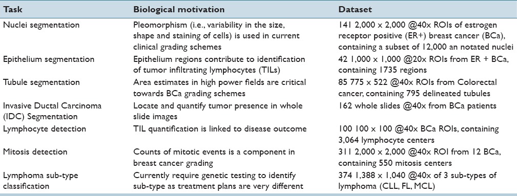
Table 1 presents a list of the seven different tasks addressed in this paper. These tasks have been chosen as they represent the ensemble of critical components necessary for most of the pertinent pathology tasks (e.g., disease grading, mitotic counting) and thus span the current challenges in the DP image analysis space. This is evidenced by large numbers of papers and grand challenges, which have been proposed to address these problems.[7,29]

Table 1.

Descriptions of the digital pathology tasks undertaken in this tutorial using seven different use cases

Segmentation and Detection Tasks

A segmentation task is defined as the requirement of delineating an accurate boundary for histologic primitives (i.e., nuclei, epithelium, tubules, and IDC) so that precise morphological features can be extracted. Detection tasks (i.e., lymphocyte and mitosis detection) are different from segmentation tasks in that the goal is typically to simply identify the center of the primitive of interest and not explicitly extract the primitive contour or boundary. Segmentation typically tends to be more challenging than detection, especially in the cases where the primitives of interest have multiple possible manifestations (e.g., mitotic cycles). Thus, a single monolithic classifier or model may not be able to capture the full range of diversity in presentation (i.e., the constellation of visual queues and features used to identify a particular histologic primitive).

Tissue-Based Classification Task

Another set of use cases we tackle in this paper is tissue level classification (i.e., lymphoma subtype identification). As opposed to explicitly identifying individual tissue-based primitives (e.g., mitoses, nuclei) and trying to identify primitive specific features to make predictions regarding tissue class, an alternative strategy is to directly learn the set of features representative of the tissue class via DL. The DL classifier could thus be trained to self-discover the nuanced disease patterns within each class. This approach thus obviates the need for explicit primitive identification and provides a more direct pathway to the final classification while not at the same time requiring a comprehension of the (potentially unknown) domain specific relationships of the primitives. In fact, in this setting, the DL approach only needs the image patches which have been tagged with the class label to learn the most discriminating representations for class separability.

Manual Annotation for Ground Truth Generation

Well annotated exemplars are an important prerequisite for DL schemes; unfortunately, the main challenge in performing any digital histopathology work is to obtain high-quality annotations. These ground truth annotations, typically done by an expert, involves delineating object boundaries or annotating pixels corresponding to a region or tissue of interest. In computational approaches, this level of annotation precision is critical so that supervised classification systems, and more specifically learn-from-data approaches (where domain knowledge is not explicitly implemented in the algorithm), can be optimized. Generating these annotations, though, is a cumbersome and laborious process, and often quite onerous, due to the large amount of time and effort needed. For example, the nuclei annotation dataset used in this work took over 40 hours to annotate 12,000 nuclei, and yet represents only a small fraction of the total number of nuclei present in all images.

There have been discussions previously in the literature,[9,30] regarding the challenges associated with supervised learning classifiers that have to rely on large swathes of deeply annotation data. The findings from[30] show that metrics computed from a single resolution appear to degrade at a finer resolution, not because the tissue classifier presented was performing worse. On the contrary, the classifier became so sophisticated at the higher magnification that it began to tease apart regions that were too subtle to be captured by an expert approximate delineations [a similar situation is shown in Figure 5]. A large contributory reason is the fact that pathologists are typically not available to perform the large amounts of laborious manual annotations at the high resolutions needed for training and evaluating supervised object detection and classification algorithms. As a result, annotations are (a) rarely pixel level precise, (b) usually done at a lower magnification, and (c) tend to contain numerous false positives and negatives. For example, the annotation of the IDC dataset took place at ×2, while there are many subregions visible at ×5 and ×10 that are clearly not IDC, but since the delineation happens quickly and at a high level, those regions are falsely included in the positive class.

Figure 5.

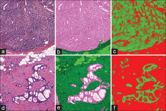
Epithelium segmentation output as produced by our approach where original images in (a and d) have their associated ground truth in (b and e) overlaid. We can see that the results from the deep learning, in (c and f), that a pixel level metric is perhaps not ultimately suited to quantify this task as deep learning is better able to provide a pixel level classification, intractable for a human expert to parallel

There can also be an issue with the ambiguity naturally present in biological images, especially where three-dimensional (3D) objects are represented in 2D, further confounding the annotation process. For example, annotating clumps or overlapping nuclei is a challenge since it is not always clear where the boundaries between intersecting nuclei lie. This is an unfortunate artifact of tissue sectioning and representation of fundamentally 3D tissue sections as a 2D planar image on a glass slide. In the discussion section below, we discuss an approach that aims to optimize the process of ground truth generation and annotation construction.

DEEP LEARNING METHODS

This section is divided into two parts. The first sub-section discusses the typical workflow used when applying DL to a DP image analysis task. The second subsection briefly describes the components typically used in constructing a DL architecture (i.e., network); instantiated as the popular CIFAR-10 version of AlexNet.[26]

Overview of Deep Learning Workflows

The DL approach employed in conjunction with the 7 use cases can be thought of as comprising the following four high-level modules.

Casting

Typically, one needs to make various decisions to design an appropriate network such as input patch size, number of layers, and convolutional attributes. We attempt to mitigate this dependency by instead opting to leverage the popular and successful AlexNet network (described below). The main reasons for using an existing architecture are 2-fold. First, finding the most successful network configuration for a given problem can be a difficult challenge given the total number of possible configurations one could avail of and also the concomitant amount of time for training and testing the network. By choosing an existing proven network, we can measure the performance of other configurations against a known benchmark. Second, since the patch size of 32 × 32 is associated with a well-known image benchmark challenge CIFAR-10,[31] and since we use a popular open-source DL framework (Caffe),[25] we create a situation by which future upgrades are essentially obtained for “free.” As newer, more efficient/accurate networks and training produces become available and integrated into Caffe, they can be directly leveraged. If we were to design our own network, without regard to input sizes and software, we would require significant upkeep to leverage any future advances in DL techniques.

Patch generation

Once the network is defined, which involves locking down input sizes, image patches need to be generated to construct the training and validation sets. This stage requires modest domain knowledge in order to ensure a good representation of diversity in the training set. Since our chosen network has limited discrimination ability (drastically reducing the likelihood of over-fitting the model), selecting appropriate image patches for the specific task could have a dramatic effect on the outcome. Especially in the domain of histopathology, there can be substantial variance present within a single target class, such as nuclei. This is especially pronounced in breast cancer nuclei, where nuclear areas can vary upwards of 200% between nuclei. Ensuring that a sufficiently rich set of exemplars is extracted from the images is perhaps one of the most key aspects of effectively leveraging and utilizing a DL approach. In Section 5: Use Cases, we present a detailed description of approaches that can allow for tailoring of training sets toward specific tasks.

Training

The training procedure for all tasks is essentially the same and follows the well-established paradigm laid out in.[32] This strategy utilizes a stochastic gradient descent approach, with a fixed batch size, (a) a series of mean corrected image patches are introduced to the network over a series of epochs, (b) an error derivative calculated, and (c) back-propagated through the network by updating the network weights. The learning rate is annealed over time so that a local minimum is reached. The resulting learned weights (i.e., the model) are stored to be used later at test time.

Testing

By submitting image patches to the network, of the same size used during training, we obtain a class prediction from the learned model.

Review of AlexNet Network Architecture

Although a full DL primer is out of the scope of this paper, we briefly discuss the components which make up the popular AlexNet and then follow on by describing the full network. We strongly encourage the reader to review,[26,27] for a complete understanding of the network. We assume the input image to be of size w × w × c, where w is both the width and height and c is the number of channel. In addition, one represents grayscale, and three represents red-green-blue.

Convolutional layer

This layer type takes a square kernel of size k × k, which is smaller than the input w, and is then convolved with the image to obtain network activations. A number of these kernels are learned such that they minimize the training error function (discussed below). Due to the static nature of natural images, especially in histopathology, a single bank of filters can optimally represent the many components present in an image. A convolutional filter is often likened to a local receptor field, where spatially proximal inputs are mapped to a single value through a filter activation. Convolutional layers are interesting because they minimize the number of individual variables required (since k² <<w²), while still displaying strong representational ability. As seen in previous papers,[33] the first layer tends to be similar to edge detectors, Gabor filters, and other first order filters. Artificially augmenting an image to a specified size (i.e., padding) often takes place to ensure favorable computational properties, such as the number of elements being processing coinciding with a power of 2 for improved GPU efficiency. Padding can be done by appending zeros but often times involve simply mirroring adjacent pixels. In addition, there is an optional stride component which specifies the intervals at which to apply the filter. Output of this is of size:

Pooling layer

These layers are used as a way of summarizing the information created from the layer above. Two types of pooling layers are typically used, max and average, which summarize an area of k × k into either the maximal value or the mean value. The output size is computed in a manner similar to the convolutional layer.

Inner product (fully connected)

This is the traditionally fully-connected layer where every input is fed into a unique output after being multiplied by a learned weight. Inner products are easily represented by matrix multiplications of a weight matrix and the input vector to produce a vector output, which is the same size as that of the previously specified number of neurons.

Activation layer

This layer operates on each element individually (i.e., element-wise) to introduce nonlinearity into the system. In past approaches,[34] a sigmoid function was typically used, but more recent implementations[35,36] have shown that a rectified linear (ReLu) activation has more favorable properties. These properties include sparser activation, elimination of vanishing/exploding gradient issues, and more efficient computation as the underlying function consists of only a comparison, addition, and multiplication. In addition, one can argue that this type of activation is more biologically plausible,[37] allowing for more consonance with the way the human brain functions. A ReLu activation is of the form f (x) = max (0, x).

Dropout layer

Performed on the fully connected layers, dropout[38] is the process of randomly excluding different neurons during each iteration of training. This has been shown to improve generalizability of the classifier to unseen cases while also eliminating overfitting as weights cannot become co-dependent. It has been shown that simply using this procedure, which could improve the training time as additional computations are simply avoided, is on par with training multiple nets with different initialization points and averaging their resulting probabilities.

Softmax layer

The entire network is optimized to minimize a loss function. In all cases discussed here, we use the softmax loss function which computes the multinomial logistic loss of values presented to it. The purpose of using softmax, as opposed to a regular argmax function is that the softmax function has the favorable property of a smooth gradient, so that the back-propagated error is not subject to discontinuities, allowing for easier training.

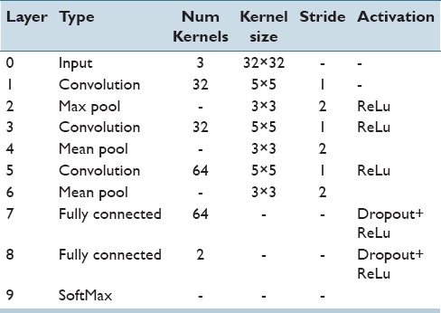
Using these components, the AlexNet describes a complete DL architecture according to Table 2. As we can see, the model accepts as input a 32 × 32 image and ends up by producing a class prediction using a softmax operation.

Table 2.

The AlexNet configurations are used in this work. The network is identical to the one provided by Caffe. The dropout network is the same except layers 7 and 8 have an additional dropout combined with the ReLu

USE CASES

We use each of the individual tasks, described in Table 1, as a vehicle to describing the unique challenges present in DP and the solutions we have implemented. We briefly discuss their clinical motivation, unique dataset characteristics, and the resulting patch generation schemas. Once the individual patches are created, in a manner that is unique to each task, the same network architecture (Section 4.2: Review of AlexNet Network Architecture) and hyperparameters are used. We present qualitative and quantitative results as well as comparisons to state-of-the-art hand-crafted classification approaches.

Deep Learning Parameters

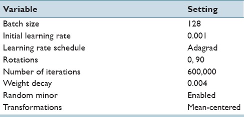
The parameters used with the stock AlexNet architecture are shown in Table 3. They were held constant to further illustrate how parameter tweaking and tuning is not strictly necessary to yield good quality results. Also to alleviate the need for an annealmeant schedule of the learning rate, we use AdaGrad[39] (which is supplied by Caffe), where optimal learning rates on a per variable basis are continuously estimated. We note that the training time is about 22 h on a Tesla M2090 GPU using CUDA 5.0 without cuDNN, and about 4 h using a Tesla K20c with CUDA 7.0 using cuDNN for all experiments as the number of iterations and mini-batch size was fixed.

Table 3.

Deep learning hyperparameter settings held constant for all experiments

A subset of the tasks below were performed using the dropout network described above. There did not exist a case where dropout improved the metrics in any of the experiments so further investigation was not performed. This is unsurprising as the original dropout paper[38] discusses that the optimal dataset size for dropout usage is smaller than the ones we have created here. As our training sets are quite large, we saw no evidence of overfitting, which further reduces the motivation for the usage of a dropout approach.

Nuclei Segmentation Use Case

Challenge

Nuclei segmentation is an important problem for two critical reasons: (a) There is evidence that the configuration of nuclei is correlated with outcome,[5] and (b) nuclear morphology is a key component in most cancer grading schemes.[40,41] A recent review of nuclei segmentation literature[42] shows that detecting these nuclei tends not to be extremely challenging, but accurately finding their borders and/or dividing overlapping nuclei is the current challenge. The overlap resolution techniques are typically applied as postprocessing on segmentation outputs, and thus outside of the scope of this paper. We have specifically chosen to look at the problem of detecting nuclei within hematoxylin and eosin (H&E) stained estrogen receptor positive (ER+) breast cancer images.

Manually annotating all of the nuclei in a single image is not only laborious but also does not generalize to all of the other variances present by other patients and their stain/protocol variances. As a result, time is better invested annotating sub-sections of each image for a number of minutes. Unfortunately, this creates a challenging situation for generating training patches. Typically, one would use the annotations as a binary mask created for the positive class, and the negation of that mask as the negative class, randomly sampling from both to create a training set. In this particular case, though while one can successfully randomly sample from the positive mask, the randomly sampling from the complement image may or may return unmarked nuclei belonging to the positive class.

Patch selection technique

An example of a standard approach for patch selection could involve selecting patches from the positive class, and using a threshold on the color-deconvolved image[43] to determine examples of the negative class (Examples of the patches are shown in Figure 2). This rationale is based on the fact that nonnuclei regions tend not to strongly absorb hemotoxin. Figure 2 shows that while the patches would correctly correspond to their associated class, the negative class [Figure 2a] would not be particularly informative from the perspective of training the network. The resulting network consequently has very poor performance in correctly delineating nuclei, as shown in Figure 3d, since these edges are underrepresented in the training set.

Figure 2.

Typical patches extracted for use in training a nuclear segmentation classifier. Six examples of (a) the negative class show large areas of stroma which are notably different than (b) the positive nuclei class and tend to be very easily classified. To compensate, we supplement the training set with (c) patches which are exactly on the edge of the nuclei, forcing the network to learn boundaries better

Figure 3.

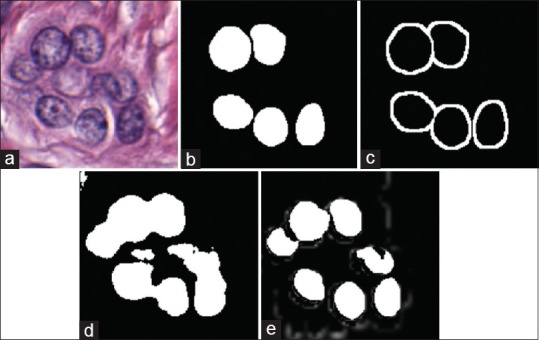
The process of creation of training exemplars to enhance the result obtained via deep learning for nuclei segmentation. The original image (a) only has (b) a select few of its nuclei annotated. This makes it difficult to find patches which represent a challenging negative class. Our approach involves augmenting a basic negative class, created by sampling from the thresholded color deconvoluted image. More challenging patches are supplied by (c) a dilated edge mask. Sampling locations from (c) allows us to create negative class samples which are of very high utility for the deep learning algorithm. As a result, our improved patch selection technique leads to (e) notably better-delineated nuclei boundaries as compared to the approach shown in (d)

To compensate, we extend the standard approach, discussed above, with intelligently sampled challenging patches for the negative class training set. Figure 3a shows an example image with its associated nuclear mask in Figure 3b. Note that only a subset of the nuclei is annotated. Using Figure 3b to identify positive pixels and the basic color deconvolution[43] thresholding approach to select random negative patches, we obtain the segmented nuclei in Figure 3d. However, as may be evidenced by the result in Figure 3d, the network is unable to accurately identify nuclear boundaries. To enhance these boundaries, an edge mask is produced by morphological dilation of Figure 3b, in turn yielding the result shown in Figure 3c. From the dilated mask, we select negative training patches, [Figure 2c] which are inherently difficult to learn due to their similarity with the positive class. We still include a small proportion of the stromal patches to ensure that these exemplars are well represented in the learning set. This patch selection technique results in clearly separated nuclei with more accurate boundaries, as seen in Figure 3e.

Results and Discussions

Each of the 5-folds in the cross-validation set had about 100 training and 28 testing images. We use a ratio of 1:1:0.3 in selecting positive patches, negative edge patches, and miscellaneous negative patches for a total of 130 k patches in the training set. We present metrics at both ×20 and ×40. For the detection rate, F-score , true positive rate (TPR) , and positive predictive value (PPV) , are calculated, where TP, FP, and FN represent true positives, false positives, and false negatives, respectively. Note that the probability map obtained via DL is thresholded at 0.5 to obtain a binary result.

Qualitatively, we can see in Figure 4 that the quantitative results correspond to the visual results. The network yields crisper nuclear boundaries that are more accurately delineated at the ×40 magnification, compared to the ×20 resolution.

Figure 4.

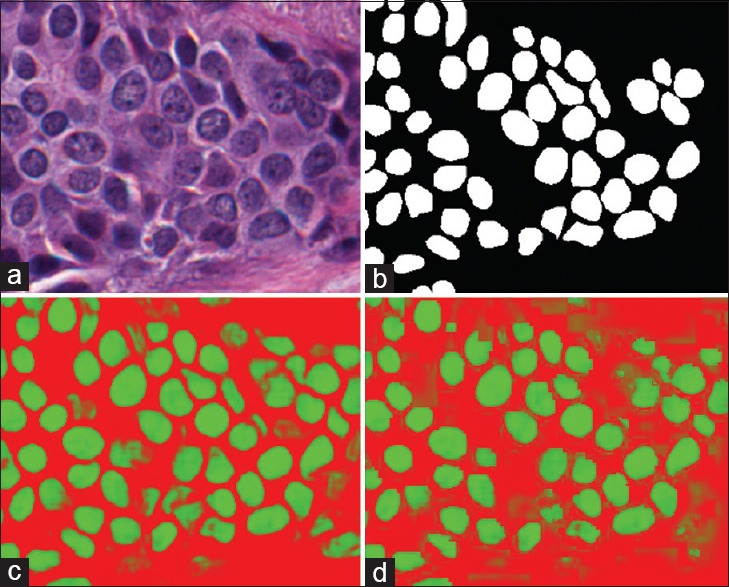
Nuclear segmentation output as produced by our approach wherein the original image in (a) is shown with (b) the associated manually annotated ground truth. When applying the network at × 40 probability map (c) is obtained, where the more green a pixel is, the higher the probability associated with it belonging to the nuclei class. The × 20 version is shown in (d)

Quantitatively, from the Table 4, we can see in all cases that the higher ×40 magnification testing performs better than the lower ×20 magnification. This is not unexpected owing to the higher strength signal embedded within the higher magnification. We also note that the detection rate, i.e., the ability to find nuclei in the image, is very high, with the network identifying 98% of all nuclei at the ×40 magnification. Dropout appears to negatively impact the metrics here. In addition, we note that in the recent review paper,[42] the performance measures are on par with several state-of-the-art nuclear detection algorithms.

Table 4.

Results for both ×20 and ×40 magnifications showing detection accuracy, F-score, true positive rate, and positive predictive value. We can see that in all cases, operating at the higher magnification produces more accurate results, though at the cost of computation time. The variances of all reported metrics were <0.001

Epithelium Segmentation Use Case

Challenge

The identification of epithelium and stroma regions is important since regions of cancer are typically manifested in the epithelium. In addition, recent work by Beck et al.[44] suggest that histologic patterns within the stroma might be critical in predicting overall survival and outcome in breast cancer patients. Thus, from the perspective of developing algorithms for predicting prognosis of disease, the epithelium-stroma separation becomes critical.

This task is unique in that it is less definitive than the more obvious tasks of mitosis detection and nuclei segmentation where the expected results are quite clear. Epithelium segmentation, especially the subcomponent of identifying clinically relevant epithelium, is typically done more abstractly by experts at lower magnifications. This has been discussed above in Section 3.3: Manual Annotation for Ground Truth Generation, but for a concrete example consider Figure 5, which shows expert annotation versus our output. Due to such discrepancies, which can make both training and evaluating difficulties, we consider an additional expert evaluation metric to validate our results.

Patch selection technique

Given that our AlexNet approach constrains input data to a 32 × 32 window, we need to appropriately scale the task to fit into this context. The general principal employed is that a human expert should be able to make an educated decision based solely on the context present in the patch supplied to the DL network. What this fundamentally implies is that we must a priori select an appropriate magnification from which to extract the patches and perform the testing. In this particular case, we downsample each image to have an apparent magnification of ×10 (i.e., a 50% reduction) so that sufficient context is available for use with the network. Networks which accept larger patch sizes could thus potentially use higher magnifications, at the cost of longer training times, if necessary.

Similar to the nuclei segmentation task discussed above, we aim to reduce the presence of uninteresting training examples in the dataset, so that learning time can be dedicated to more complex edge cases. Epithelium segmentation can have areas of fat or the white background of the stage of the microscope removed by applying a threshold at conservative level of 0.8 to the grayscale image, thus removing those pixels from the patch selection pool. In addition, to enhance the classifiers ability to provide crisp boundaries, samples are taken from the outside edges of the positive regions, as discussed above in Section 5.2: Nuclei Segmentation Use Case.

Results and Discussion

Each of the 5-fold cross validation sets has about 34 training images and 8 test images. We use a ratio of 5:5:1.5 in selecting positive patches, negative edge patches, and miscellaneous negative patches for a total of 765 k patches in the training set.

Quantitatively, we evaluate our results using the F-score after applying (a) a thresholding procedure to eliminate all the white pixels from the background, (b) an area threshold to remove all objects with an area <300 as these areas are not clinically relevant. Next, we aim to identify the optimal threshold using the 1^st fold and apply it to all other folds. In addition, we separately report the F-score of each fold the corresponding to the unique optimal threshold that was identified. These results are summarized in Table 5.

Table 5.

F-scores for epithelium versus stroma segmentation task. We can see that the optimal thresholds of each fold are close to each other as are the F-scores

We can see that the individual optimal thresholds are all very near each other. These findings appear to suggest that the network and the classifier are relatively robust to variations in the training set.

Qualitatively, from the above Figure 5, we can see that pathologists often treat this task as a higher level abstraction instead of a pixel level classification. It becomes clear in panel (f) why we exclude white pixels from the metric computation, as these gaps correspond to white background which is rarely removed manually by the pathologist (as shown in (e)). We note that we are also able to identify smaller regions which are often ignored by pathologists, most likely since they are not believed to be clinically relevant.

While visually our results appear quite similar to the original ground truth, the additional pixel level detail that the DL segmentation yields are not quite captured by the quantitative metrics, as we discussed in Section 3.3: Manual Annotation for Ground Truth Generation.

Apart from the quantitative performance measures, we also had our results reviewed by our clinical collaborator and these results were then graded on a scale of 1–5, where 1 is “poor, not fit for purpose” and 5 is “definitely fit for purpose.” On average, our images were scored a 4 with a standard deviation of 0.8. This implies that overall our results are suitable to be used in conjunction with other classification algorithms (e.g., prognosis prediction).

Interestingly, this is the first attempt, to our knowledge, to directly segment and quantify epithelium tissue in general and more specifically in breast tissue. We hope that with the release of our dataset, with annotations, other researchers will be interested in using it as a benchmark to quantify their respective segmentation approaches.

Tubule Segmentation Use Case

Challenge

The morphology of tubules is correlated with the aggressiveness of the cancer, where later stage cancers present with the tubules becoming increasingly disorganized, as seen in Figure 6. The Nottingham breast[40] cancer grading criteria divides scoring of the tubules into three categories according the area relative to a high power field of view: (i) >75%, (ii) 10–75%, and (iii) <10%. The benefits of being able to identify and segment the tubules are thus 2-fold, (a) automate the area estimation, decreasing inter-/intra-reader variances, and (b) provide greater specificity, which can potentially lead to better stratifications associated with prognosis indication.

Figure 6.

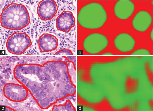
The benign tubules, outlined in red, (a) are more organized and similar, as a result the deep learning can provide very clear boundaries (b), where the stronger green indicates a higher likelihood that a pixel belongs to the tubule class. On the other hand, when considering malignant tubules (c), the variances are quite large making it more difficult for a learn from data approach to generalize to all unseen cases. Our results (d) are able to identify a large portion of the associated pixels, but can be seen providing incorrect labeling in situations where traditional structures are not present

Tubules are the most complex structures considered so far. They not only consist of numerous components (e.g., nuclei, epithelium, and lumen) but also the organizational structure of these components determines tubule boundaries. There is a very large variance in the way tubules present given the underlying aggressiveness and stage of cancer. In benign cases [Figure 6a], tubules present in a well-organized fashion with similar size and morphological properties, making their segmentation easier, while in cancerous cases [Figure 6c], it is clear that the organization structure breaks down and accurately identifying the boundary becomes challenging, even for experts. To further compound the complexity of the situation, tubules as an entity are much larger compared to their individual components, thus requiring a greater viewing area to provide sufficient context to make an accurate assessment.

Patch selection technique

In this use case, we introduce the concept of using cheap preprocessing to help identify challenging patches, which can help provide more informative and diverse exemplars to the DL system. Per image, we randomly select a number of pixels (e.g., 15,000) belonging to both classes to act as training samples, and compute a limited set of texture features (i.e., contrast, correlation, energy, and homogeneity). These features were chosen because they are available in MATLAB and are also very fast to compute. Next, we use a naïve Bayesian classifier to determine posterior probabilities of class membership for all the pixels in the image. In a matter of seconds, we are able to identify pixels which would potentially produce false positives and negatives and thus would benefit from additional representation in the DL training set. These pixels are selected based on their magnitude of confidence, such that false positives with posterior probabilities closer to 1 are selected with greater likelihood than those with .51. This approach further helps us to bootstrap our training set, by removing trivial samples, without requiring any additional domain knowledge.

Finally, knowing that benign cases are easier to segment than malignant cases, patches are disproportionally selected from malignant cases to further help with generalizability. While this dataset comes with the samples divided into benign and malignant cases, which is a valuable piece of knowledge to have ahead of time, an approach discussed in Section 5.5: Invasive Ductal Carcinoma Segmentation Use Case, could just as easily have been used to help dichotomize the training set.

Results and discussion

Figure 6 shows that benign sections of tissue do well as a result of being able to generalize well from the dataset. Malignant tubules, on the other hand, are far more abstract and tend to have the hallmarks of a tubule, such as clear epithelial ring around a lumen, less obvious making them harder to generalize to. This is potentially one of the downfalls of machine learning techniques, which make inferences from training data; when insufficient examples are provided to cover all cases expected to be viewed in testing phases the approaches begin to fail. On the other hand, in this case, especially these challenges could be addressed by providing a larger database of malignant images.

Each of the 5-fold cross validation sets has about 21 training images and 5 test images. We use a ratio of 2:1 of malignant to benign patches whereas also including rotations of 180 and 270 to the malignant training set, for a total of about 320 k training patches. The mean F-score, using a threshold of 0.5, was 0.827 ± 0.05. When we optimized the threshold on a per fold basis, the measure rose slightly to 0.836 ± 0.05. To determine if this was suitable for clinical usage, we computed the difference in area between our results and the ground truth results. When combining all the test sets together, the P = 0.33, indicating that there was no significant difference between the expected clinical grade associated with our approach versus and expert's ground truth annotation. Two state-of-the-art approaches claim 86% accuracy[45] and 0.845 object-level dice coefficient,[46] indicating that our approach is on par with others currently in the field.

Invasive Ductal Carcinoma Segmentation Use Case

Challenge

Invasive Ductal Carcinoma (IDC) is the most common subtype of all breast cancers. To assign an aggressiveness grade to a whole mount sample, pathologists typically focus on the regions which contain the IDC. As a result, one of the common preprocessing steps for automatic aggressiveness grading is to delineate the exact regions of IDC inside of a whole mount slide.

We obtained the exact dataset, down to the patch level, from the authors of[9] to allow for a head to head comparison with their state-of-the-art approach, and recreate the experiment using our network. The challenge, simply stated is can our smaller more compact network produce comparable results? Our approach is at a notable disadvantage as their network accepts patches of size 50 × 50, while ours use 32 × 32, thus being provided 60% less pixels of context to the classifier.

Patch selection technique

To provide sufficient context (as discussed above in epithelium segmentation section), the authors have down sampled their original ×40 images by a factor of 16:1, for an apparent magnification of ×2.5. We attempted three different approaches of using these 50 × 50 patches, and casting them into our 32 × 32 solution domain:

Resizing

Using the entire 50 × 50 patch, we resize it down to 32 × 32.

Cropping: Each 50 × 50 image was cropped to a 32 × 32 sub-patch from exactly the center to ensure that the class label was correctly retained.

Cropping + additional rotations: To compensate for the heavily imbalanced training set, where the negative class is represented over 3 times as much, we artificially oversample the positive class by adding additional rotations. Since the provided patches are 50 × 50, we can rotate them around the center of the image origin, and still crop out a 32 × 32 image. As a result, we use rotations of 0, 45, 90, 135, 180 degrees, along with their mirrors to the training set for the positive class. We continue to use only the 2 rotations for the negative class as before. The totals patches available for training are about 157 k for the positive set and about 167 k for the negative set, nearly balancing the classes.

Results and discussion

Qualitatively, we can see from Figure 7 that our results are quite similar to.[9] While the pathologist annotations are shown in green in Figure 7a, we note that in our results, the upper right corner is not a false positive, but simply a region underannotated by the pathologist. As we discussed above in Section 3.3: Manual Annotation for Ground Truth Generation, this continues to be one of the challenges in DP; computer algorithms can often be more fine grained as the computation time is cheap while performing the same level of annotation for a pathologist is simply too laborious.

Figure 7.

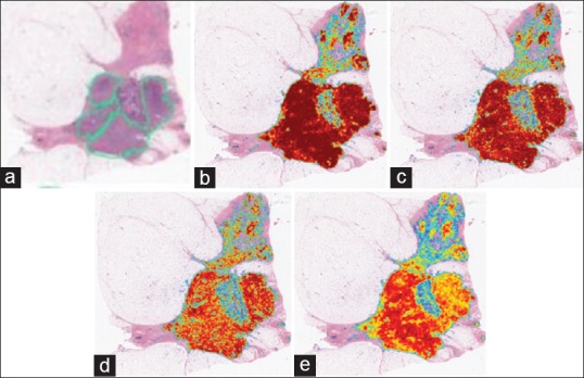
Invasive ductal carcinoma segmentation where we see the original sample (a) with the pathologist annotated region shown in green. From (b) we can see the results generated by the resizing approach, (c) shows the same results without resizing, (d) shows the output when resizing and balancing the training set and (e) finally resizing with dropout, where the more red a pixel is, the more likely it represents an invasive ductal carcinomas pixel. We note that the upper half of the image actually contains true positives which were not annotated by the pathologist

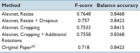
Quantitatively, we present the F-score and the balanced accuracy for our methods to compare against[9] in Table 6. We can see that using our net provides a better F-score and also a slightly higher accuracy balance. Interestingly, resizing the images seems to produce the best results indicating that the selected field of view is critical to obtaining better results. While cropping the images produces better resolution patches, the field of view is smaller, most likely making certain areas tricky to differentiate without neighborhood information. Again, we note that dropout did not provide any improvement in generalization during test time.

Table 6.

F-score and balance accuracy for the various approaches. We note that resizing the larger patches to fit into our existing framework provided the best results, as well as improving upon previous results using the same dataset

Lymphocyte Detection Use Case

Challenge

Lymphocytes, a subtype of white blood cells, are an important part of the immune system. Lymphocytic infiltration is the process by which the density of lymphocytes greatly increases at sites of disease or foreign bodies, indicating an immune response. A stronger immune response has been highly correlated to better outcomes in many forms of cancer, such as breast and ovarian. As a result, identifying and quantifying the density and location of lymphocytes has gained a lot of interest recently, particularly in the context of identifying which cancer patients to place on immunotherapy.

Lymphocytes present with a blue tint from the absorption of hemotoxylin, their appearance similar in hue to nuclei, making them difficult to differentiate in some cases. Typically, though, lymphocytes tend to be smaller, more chromatically dense, and circular. In this particular use case, our goal was to identify the center of lymphocytes, making this a detection problem (see Section 3: Digital Pathology Tasks Addressed).

Patch selection technique

At the original ×40 magnification, the average size of a lymphocyte is approximately 10 pixels in diameter, much smaller than the 32 × 32 patches used by our network. The focus here is on identifying lymphocytes without focusing on the surrounding tissue if the patches were to be extracted at ×40, only 10% of the input pixels would be of interest. The other 90% of the input pixels would eventually learn to be ignored by the network. This would have the unfortunate effect of reducing the discriminative ability of the network. Thus, to increase the predictive power of the system, we artificially resize the images to be ×4 as large, so that the entire input space, when centered around a lymphocyte, contains lymphocyte pixels, allowing more of the weights in the network to be useful.

Positive class exemplars are extracted by randomly sampling locations from a 3 × 3 region around the supplied centers of each lymphocyte. The selection of the negative class proceeds as follows, (a) a naïve Bayesian classifier is trained on 1000 randomly selected pixels from the image to generate posterior class membership probabilities for all pixels in the image, (b) for all false positive errors, the distance between the false positive pixels and the closest true positive pixels is computed, (c) iteratively, the pixel with the greatest distance between the false positive and true positive errors is chosen so that negative image patches can be generated from those locations. Since there are few positive samples available, the training set is augmented by adding additional rotations.

At test time, the posterior probabilities are computed for every pixel in the test image. To identify the location most likely to be the center of a lymphocyte, a convolution is performed with a disk kernel and the probability output so that the center of the probably regions are highlighted. Iteratively, the highest point in the image is taken as center and a radius is cleared, which is the same size as a typical lymphocyte to prevent multiple centers from being identified for the same lymphocyte.

Results and discussion

Each of the 5-fold cross validation sets has about 80 training and 21 test images. We use a ratio of 1:1 for the positive and negative classes, while also including rotations of 180° and 270° to the positive training set due to them being under-represented, for a total of about 700 k training patches. We used a single fold to optimize the variables (disk clearing, convolution disk size, and threshold) and applied them unchanged to the other 4 folds. The optimal threshold was found to be at 0.7066, convolution disk size of 6 and clearing disk of size 28. The mean F-score was found to be 0.90 ± 0.01, mean TPR 0.93 ± 0.01 and PPV of 0.87 ± 0.02, demonstrating a favorable comparison to the states of the art which show (a) a TPR of 86% and PPV of 64%[47] and (b) F-score of 88.48.[48] Qualitatively, as shown above in Figure 8, we are able to detect most of the lymphocytes. The dataset itself has lymphocytes on the borders of the image, often times with over 50% of the lymphocyte not being visible [as shown above in Figure 8a], making detection difficult for such edge pixels.

Figure 8.

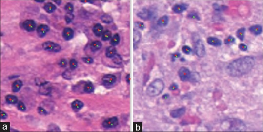
Lymphocyte detection result where green dots are the ground truth, and red dots are the centers discovered by the algorithm. The image on the left (a) has 21 TP/2 FP/0 FN. The false positives are on the edges, about 1 o’clock and 3 o’clock. The image on the right (b) one has 11 TP/1 FP/2 FN. We can see the false negatives are quite small and not very clear making it hard to detect them without also encountering many false positives. The only false positive is in the middle at around 7 o’clock though this structure does look “lymphocyte-like

Mitosis Detection Use Case

Challenge

The number of mitoses present per high power field is an important aspect of breast cancer grade. Typically, the more aggressive the cancer, the faster the cells are dividing which can be approximated by counting the mitotic events in a histologic snapshot. The current grading scheme divides the mitotic counts into three categories per 10 high-power fields, (i) ≤7 mitoses, (ii) 8−14 mitoses, and (iii) ≥15 mitoses. This is an active area of interest with a number of competitive grand challenges taking place in this space.[6,7,8]

In practice, pathologists rely on changing the focal length of an optical microscope to visualize 3 dimensionally the mitotic structure, allowing them to eliminate false positives from their estimates. As such, accurately identifying mitosis on a 2D digital histology image is very difficult but highly sought after as it would allow for the automatic interrogation of existing large, long-term, repositories. An open question in the field is trying to determine the minimal amount of accuracy necessary for clinical usage.

Patch selection technique

Since the network is smaller than the one used in[8] (32 × 32 as compared to 101 × 101), we modified and extended the approach in[8] accordingly. In order to provide enough context for each of the patches, we perform all operations at ×20 apparent magnification, such that an entire mitotic figure can be captured within a single image patch. This is most important in cases where the mitosis is in the anaphase or telophase [Figure 9c], and the coordinates provided by the ground truth are actually in the middle of the two new cells.

Figure 9.

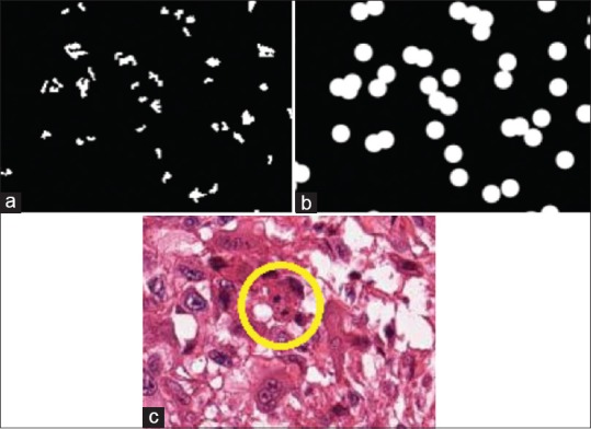
Result of deep learning for mitosis detection, where the blue ratio segmentation approach is used to generate the initial result in (a). We take this input and dilate it to greatly reduce the total area of interest in a sample. (b) In the final image, (c) we can see that the mitosis is indeed located in the middle of the image, included our computational mask. We can see that the mitosis is in the telophase stage, such that the DNA components have split into two pieces (in yellow circle), making it more difficult to identify

For the positive class we take each known mitosis location, and use a 4-pixel radius around it to construct the corresponding training patch. Since there are very few training pixels available, we add a large number of rotations to augment the training set, in this case, rotations of 0, 45, 90, 135, 180, 215, 270 degrees.

For the negative class, and to reduce both computational time, and in order to improve the selection of image patches, we leverage a well-known segmentation technique termed blue-ratio segmentation since there is evidence that mitoses are highlighted in regions identified by the blue ratio segmentation scheme [Figure 9a].[49,50] The results of the blue ratio segmentation approach are dilated into a 20 disk radial mask [Figure 9b]. This creates regions from which we will sample the negative patches, as it enables the natural elimination of trivial examples from the learning process. We sample 2.5 times as many patches as positive patches but only rotate each of them in 0, 90, 180, 270 degrees, so that we have more unique patches instead of simply rotated images.

Subsequently and modeled on the approach in,[8] a naïve Bayesian is employed in order to compute the probability masks for the training set. A new DL network is then trained by oversampling from the false positives produced by the first network. This is done so that we can focus the classification power of the network on the most difficult cases. In particular, for the ground truth, we use the same positive class selection except we increase the number of rotations to every 15°. For the negative class, we only consider probabilities which are in the blue ratio generated mask, and sample those according to their weights. This makes it possible to select pixels which were, incorrectly, strongly believed to be a mitotic event. This approach resulted in approximately 600 k patches for the first stage of training and 4 million patches for the second stage of training. To identify the final locations of the mitoses, we convolve the image with a kernel disk and identify a mitotic event as those image locations identified as being above a certain probability threshold.

Results and discussion

Our 5-fold analysis produced a mean F-score of 0.37 ± 0.2 when using the first round classifier and 0.54 ± 0.1 when using the second trained classifier, indicating a substantial improvement when using two sequential DL networks, where the second DL network is trained based off the false positive errors identified by the first DL network. Our F-scores are comparable to the state-of-the-art and only marginally lower than the winner of a recent grand challenge competition on mitosis detection.[8] The winners of that grand challenge (F-score = 0.61) use a 101 × 101 size patches which operates at ×40, and thus contains increased classification power as compared to our 32 × 32 approach at ×20. In our runs of cross-validation, the thresholds varied significantly across different folds suggesting that an independent validation set is needed for evaluating the trained network. Typical false and true positives can be seen in Figure 10a and b, respectively.

Figure 10.

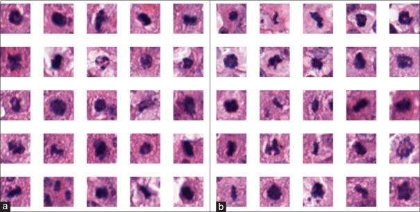
False positive samples of mitoses (a) with (b) true positive samples on the right. We can see that in many cases the two classes are indistinguishable from each other in the two-dimensional plane, thus requiring the common practice of focal length manipulation of the microscope to determine which instances are truly mitotic events

Lymphoma Subtype Classification Use Case

Challenge

The NIA curated this dataset to address the need of identifying three sub-types of lymphoma: Chronic lymphocytic leukemia (CLL), follicular lymphoma (FL), and mantle cell lymphoma (MCL). Currently, class-specific probes are used in order to reliably distinguish the subtypes, but these come with additional cost and equipment overheads. Expert pathologists specializing in these types of lymphomas, on the other hand, have shown promise in being able to differentiate these sub-types on H&E, indicating that there is the potential for a DP approach to be employed. A successful approach would allow for more consistent and less demanding diagnosis of this disease. This dataset was created to mirror real-world situations and as such contains samples prepared by different pathologists at different sites. They have additionally selected samples which contain a larger degree of staining variation than one would normally expect [Figure 11].

Figure 11.

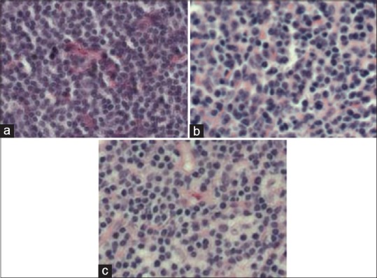
Exemplars taken from the (a) chronic lymphocytic leukemia, (b) follicular lymphoma, and (c) mantle cell lymphoma classes used in this task. There is notable staining difference across the three samples. Also, it is not intuitively obvious what the characteristics are which should be used to classify these images

This use case represents the only classification use case of this manuscript: Attempting to separate images into 1 of 3 sub-types of lymphoma. In the previous tasks, we were looking at primitives and attempting to segmented or detect them. In this case, though, a high-level approach is taken, wherein we provide whole tissue samples to have the DL learn unique features of each class.

Patch selection technique

To generate training patches, a naïve approach was used. Images were split into 36 × 36 sub-patches with a stride of.[32] Caffe has the ability, at training time, to randomly crop out smaller 32 × 32 patches from the larger ones provided, artificially increasing the dataset. This approach could not be used in other tasks because there was no guarantee that the center pixel would retain the appropriate class label (consider an edge pixel of nuclei, an arbitrary translation could potentially change its underlying class). During testing time, patches were extracted using the same methodology, and a voting scheme per subtype was used where votes were aggregated based on the DLs output per patch. In a winner-take-all, the class with the highest number of votes became the designated class for the entire image.

Results and discussion

Each of the 5-fold cross validation sets had 300 training images and 75 test images, for a total of about 825 k training patches. The mean accuracy is 96.58% ±0.01% (on average 2.6 misclassified images in 75 tests). This is over a 10% improvement from the software package, wnd-chrm,[51] where the dataset was also used. Interestingly, both approaches encode no domain knowledge.

In the cases where images were incorrectly classified, there tends to be an overall poor quality of the slide, which would have resulted in either a rescan or a removal. For example, in Figure 12, the images have significant artifacts which likely caused its misclassification. The voting for these types of images shows 814 patches assigned to the CLL category, 562 patches to the FL category, and 0 patches to the MCL category, a strong indication of uncertainty. When this is compared to other images, for example, in the FL category, the scoring is {5, 1357, 14}, respectively. This indicates that in the case where there is not a landslide voting victory, the slide should be reviewed manually.

Figure 12.

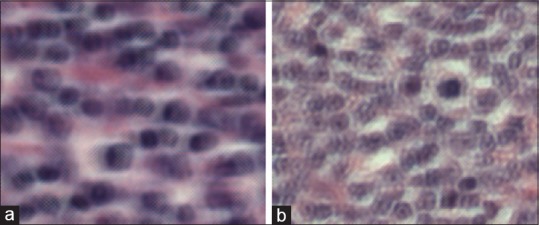
(a and b) Misclassified image belonging to the follicular lymphoma subtype. We can see that when magnified, there appears to be some type of artifact created during the scanning process. It is not unreasonable to think that upon seeing this a clinician would ask for it to be rescanned

DISCUSSION

There are a few insights which can be gleaned from the experiments involving the use cases. First, there was no situation which dropout had improved the resulting metrics. Srivastava et al.[38] performed rigorous quantitative evaluation identifying dataset sizes which might benefit from dropout. Our datasets are larger than the recommended sizes discussed in their paper and are thus likely large enough that we do not suffer from overfitting. This potentially limited the utility of dropout in our use cases.

Second, it is of the utmost importance to select an appropriate magnification for each task. The rule of thumb we employed is that a human expert should be able to make the correct assessment given only the context presented in a patch. For this reason, tasks such as the epithelium segmentation were performed at very low magnification, while nuclei edge detection was performed at higher magnification. By the same token, if too low of magnification is selected for a task, only a few pixels supply the context needed for the class identification. As a result, the network becomes less powerful as the noncontext pixels have no use and yet still consume input variables.

Third, a majority of the work in this paper focused on finding simple, albeit robust ways of identifying challenging exemplars for training, in other words, those exemplars that would be most informative to the DL network. In situations where random selection was solely utilized, there are too many instances of trivial exemplars that ended up being selected, exemplars that did not enhance the learning capability of the network (e.g., nuclei segmentation task). Another technique for identifying important patches was to use a 2-stage classification stage (i.e., mitosis detection and lymphocyte detection), where false positives and negatives from the first round classifier were oversampled to form the second training set.

In addition, due to the nature of DL, where inferences are derived from data, improving ground truth annotations so that they are precise to the pixel level, would likely further improve the results. Figure 5 illustrates the difference between a typical manual segmentation of a pathologist versus a pixel level output produced by an algorithm. DL has the potential to provide a first pass ground truth annotation of very high quality, thus allowing domain experts such as pathologists to solely focus on correcting errors made by the DL network.

Finally, while we have mentioned comparable current state-of-the-art metrics where applicable, we note that datasets complexity can vary greatly in digital histopathology, perhaps more so than other domains, making a direct comparison difficult if not impossible unless a single benchmark dataset used. Consequently, we are releasing our datasets and annotations, online for usage, and review by the community in hopes of creating more standardized benchmarks. However, we wish to emphasize that a single unified DL framework that was employed with little to no modifications across a variety of different use cases yielded results that compared favorably with the best-reported results for each of those domains, a remarkable result in light of the fact that little to no domain specific information was invoked.

CONCLUSION

We have shown how DL can be a valuable unifying tool for the DP domain due to its innate ability to learn useful features directly from data. Via seven use cases, (a) nuclei segmentation, (b) epithelium segmentation, (c) lymphocyte detection, (d) mitosis detection, and (e) lymphoma classification, we have outlined a guide containing the necessary insights for bridging the current knowledge gap between DL approaches and the DP domain. In particular, we have shown that a common, practical, and publicly available software framework can perform on par, or better, than several state-of-the-art classification approaches for several digital histopathology tasks. Using this tutorial in conjunction with our supplemental online resources, we believe researchers can rapidly augment their current tools by leveraging DL for their specific histological needs.

We do however acknowledge that this tutorial and the associated framework did have some limitations. At test time, using the mean of the output from many rotations of the same patch has been shown to further reduce the variance of the output.[8] Others have shown 15 that training multiple networks, with the same or different architectures, can work well in the form of a consensus of experts voting scheme, as each network is initialized randomly and does not derive the same local minimum.

Given that all of the approaches presented in this tutorial did not explicitly and specifically invoke domain specific information, additional improvements could be made by invoking additional handcrafted or domain pertinent features. For example, the nuclei segmentation approach discussed does not address the need to split clustered cells, but such postprocessing approaches tend to require the well-defined boundaries that our approaches provide. Hand-crafted features can also be used in parallel with DL to improve the quality of the classifier.[50] Conversely, recently presented approaches[52,53] can potentially reverse engineer DL models to determine what relationships were discovered and thus supply valuable insights to the specific problem domain.

Computational efficiency is also a concern, given such large images. Hierarchical approaches have been discussed which greatly limit the number of patches, which must be classified by the network, improving efficiency.[54] In addition, approaches such as blue-ratio segmentation or color deconvolution could serve as a preprocessing step to identify locations for subsequent application of a DL network, for instance in the detection of nuclei.

The approaches presented here are not intended to be a final ending point towards all histological problems, but a surprisingly robust jumping off point for further research. In fact, given that the mitosis benchmark results, it is evident that a 32 × 32 network is not the optimal framework for all challenges. Yet with the source code and data at hand, it becomes possible to begin training and employing DL networks very rapidly and begin to modulate the approaches as appropriate for task specific settings.

Financial Support and Sponsorship

Research reported in this publication was supported by the National Cancer Institute of the National Institutes of Health under award numbers 1U24CA199374-01, R21CA167811-01, R21CA179327-01; R21CA195152-01 the National Institute of Diabetes and Digestive and Kidney Diseases under award number R01DK098503-02, the DOD Prostate Cancer Synergistic Idea Development Award (PC120857); the DOD Lung Cancer Idea Development New Investigator Award (LC130463), the DOD Prostate Cancer Idea Development Award; the Ohio Third Frontier Technology development Grant, the CTSC Coulter Annual Pilot Grant, the Case Comprehensive Cancer Center Pilot Grant VelaSano Grant from the Cleveland Clinic the Wallace H. Coulter Foundation Program in the Department of Biomedical Engineering at Case Western Reserve University.

Conflicts of Interest

Dr. Madabhushi is an equity holder in Elucid Bioimaging and in Inspirata Inc.. He is also a scientific advisory consultant for Inspirata Inc and also sits on its scientific advisory board. He is also an equity holder in Inspirata Inc. Additionally his technology has been licensed to Elucid Bioimaging and Inspirata Inc. He is also involved in a NIH U24 grant with PathCore Inc.

REFERENCES

- 1.Gurcan MN, Boucheron LE, Can A, Madabhushi A, Rajpoot NM, Yener B. Histopathological image analysis: A review. IEEE Rev Biomed Eng. 2009;2:147–71. doi: 10.1109/RBME.2009.2034865. [DOI] [PMC free article] [PubMed] [Google Scholar]
- 2.Veta M, Pluim JP, van Diest PJ, Viergever MA. Breast cancer histopathology image analysis: A review. IEEE Trans Biomed Eng. 2014;61:1400–11. doi: 10.1109/TBME.2014.2303852. [DOI] [PubMed] [Google Scholar]
- 3.Bhargava R, Madabhushi A. A review of emerging themes in image informatics and molecular analysis for digital pathology. [Last accessed on 2016 Apr 19];Annu Rev Biomed Eng. 2016 18 doi: 10.1146/annurev-bioeng-112415-114722. [DOI] [PMC free article] [PubMed] [Google Scholar]
- 4.Lewis JS, Jr, Ali S, Luo J, Thorstad WL, Madabhushi A. A quantitative histomorphometric classifier (QuHbIC) identifies aggressive versus indolent p16-positive oropharyngeal squamous cell carcinoma. Am J Surg Pathol. 2014;38:128–37. doi: 10.1097/PAS.0000000000000086. [DOI] [PMC free article] [PubMed] [Google Scholar]
- 5.Basavanhally A, Feldman M, Shih N, Mies C, Tomaszewski J, Ganesan S, et al. Multi-field-of-view strategy for image-based outcome prediction of multi-parametric estrogen receptor-positive breast cancer histopathology: Comparison to oncotype DX. J Pathol Inform. 2011;2:S1. doi: 10.4103/2153-3539.92027. [DOI] [PMC free article] [PubMed] [Google Scholar]
- 6.Veta M, van Diest PJ, Willems SM, Wang H, Madabhushi A, Cruz-Roa A, et al. Assessment of algorithms for mitosis detection in breast cancer histopathology images. Med Image Anal. 2015;20:237–48. doi: 10.1016/j.media.2014.11.010. [DOI] [PubMed] [Google Scholar]
- 7.Roux L, Racoceanu D, Loménie N, Kulikova M, Irshad H, Klossa J, et al. Mitosis detection in breast cancer histological images An ICPR 2012 contest. J Pathol Inform. 2013;4:8. doi: 10.4103/2153-3539.112693. [DOI] [PMC free article] [PubMed] [Google Scholar]
- 8.Ciresan DC, Giusti A, Gambardella LM, Schmidhuber J. Mitosis detection in breast cancer histology images with deep neural networks. Med Image Comput Comput Assist Interv. 2013;16(Pt 2):411–8. doi: 10.1007/978-3-642-40763-5_51. [DOI] [PubMed] [Google Scholar]
- 9.Cruz-Roa A, Basavanhally A, González F, Gilmore H, Feldman M, Ganesan S, et al. Automatic detection of invasive ductal carcinoma in whole slide images with convolutional neural networks. SPIE Medical Imaging. 2014;9041:904103-904103-15. [Google Scholar]
- 10.Chen T, Chefd’hotel C. Deep learning based automatic immune cell detection for immunohistochemistry images. In: Wu G, Zhang D, Zhou L, editors. Machine Learning in Medical Imaging. (Lecture Notes in Computer Science) Vol. 8689. Springer International Publishing; 2014. pp. 17–24. [Google Scholar]
- 11.Goodfellow IJ, Warde-Farley D, Lamblin P, et al. Pylearn2: A machine learning research library. arXiv preprint arXiv: 1308.4214. 2013 [Google Scholar]
- 12.Bastien F, Lamblin P, Pascanu R, Bergstra J, Goodfellow IJ, Bergeron A, et al. “Theano: New Features and Speed Improvements.” Deep Learning and Unsupervised Feature Learning NIPS 2012 Workshop. 2012 [Google Scholar]
- 13.LeCun Y, Bottou L, Orr G, Muller K. Efficient backprop. In: Orr G, Müller KR, editors. Neural Networks: Tricks of the Trade. Springer; 1998. [Google Scholar]
- 14.Montavon G, Orr GB, Müller K, editors. Neural Networks: Tricks of the Trade. (Lecture Notes in Computer Science) 2nd ed. Vol. 7700. Springer; 2012. [Google Scholar]
- 15.Ciresan D, Giusti A, Gambardella LM, Schmidhuber J. Deep neural networks segment neuronal membranes in electron microscopy images. In: Pereira F, Burges C, Bottou L, Weinberger K, editors. Advances in Neural Information Processing Systems 25. Curran Associates, Inc; 2012. pp. 2843–51. [Google Scholar]
- 16.Kainz P, Pfeiffer M, Urschler M. Semantic Segmentation of Colon Glands with Deep Convolutional Neural Networks and Total Variation Segmentation. CoRR, Vol. abs/151106919. 2015 doi: 10.7717/peerj.3874. [DOI] [PMC free article] [PubMed] [Google Scholar]
- 17.Maqlin P, Thamburaj R, Mammen J, Manipadam M. Automated nuclear pleomorphism scoring in breast cancer histopathology images using deep neural networks. In: Prasath R, Vuppala AK, Kathirvalavakumar T, editors. Mining Intelligence and Knowledge Exploration. (Lecture Notes in Computer Science) Vol. 9468. Springer International Publishing; 2015. pp. 269–76. [Google Scholar]
- 18.Sirinukunwattana K, Raza S, Tsang YW, Snead D, Cree I, Rajpoot N. Locality sensitive deep learning for detection and classification of nuclei in routine colon cancer histology images. IEEE Trans Med Imaging. 2016 doi: 10.1109/TMI.2016.2525803. [DOI] [PubMed] [Google Scholar]
- 19.Zhou Y, Chang H, Barner KE, Parvin B. Nuclei Segmentation via Sparsity Constrained Convolutional Regression. Biomedical Imaging (ISBI), 2015 IEEE 12th International Symposium on; April. 2015:1284–7. doi: 10.1109/ISBI.2015.7164109. [DOI] [PMC free article] [PubMed] [Google Scholar]
- 20.Xu J, Xiang L, Liu Q, Gilmore H, Wu J, Tang J, et al. Stacked sparse autoencoder (SSAE) for nuclei detection on breast cancer histopathology images. IEEE Trans Med Imaging. 2016;35:119–30. doi: 10.1109/TMI.2015.2458702. [DOI] [PMC free article] [PubMed] [Google Scholar]
- 21.Xu Y, Jia Z, Ai Y, Zhang F, Lai M, Chang EIC. Deep Convolutional Activation Features for Large Scale Brain Tumor Histopathology Image Classification and Segmentation. Acoustics, Speech and Signal Processing (ICASSP), 2015 IEEE International Conference on; April. 2015:947–51. [Google Scholar]
- 22.Sirinukunwattana K, Ahmed Raza S, Tsang Y, Snead D, Cree I, Rajpoot N. A spatially constrained deep learning framework for detection of epithelial tumor nuclei in cancer histology images. In: Wu G, Coupé P, Zhan Y, Munsell B, Rueckert D, editors. Patch-Based Techniques in Medical Imaging. Vol. 9467. (Lecture Notes in Computer Science) Springer International Publishing; 2015. pp. 154–62. [Google Scholar]
- 23.Xu J, Luo X, Wang G, Gilmore H, Madabhushi A. A deep convolutional neural network for segmenting and classifying epithelial and stromal regions in histopathological images. Neurocomputing. 2016;191:214–23. doi: 10.1016/j.neucom.2016.01.034. [DOI] [PMC free article] [PubMed] [Google Scholar]
- 24.Ertosun MG, Rubin DL. Automated grading of gliomas using deep learning in digital pathology images: A modular approach with ensemble of convolutional neural networks. AMIA Annu Symp Proc. 2015;2015:1899–908. [PMC free article] [PubMed] [Google Scholar]
- 25.Jia Y, Shelhamer E, Donahue J, Karayev S, Long J, Girshick R, et al. Caffe: Convolutional Architecture for Fast Feature Embedding. arXiv preprint arXiv: 1408.5093. 2014 [Google Scholar]
- 26.Krizhevsky A. Convolutional Deep Belief Networks on Cifar-10. 2010. [Last accessed on 2016 Mar 30]. Available from: https://www.cstoronto.edu/~kriz/conv-cifar10-aug2010.pdf .
- 27.Krizhevsky A, Sutskever I, Hinton GE. Imagenet classification with deep convolutional neural networks. In: Pereira F, Burges C, Bottou L, Weinberger K, editors. Advances in Neural Information Processing Systems 25. Curran Associates, Inc; 2012. pp. 1097–105. [Google Scholar]
- 28.Janowczyk A. Deep Learning for Digital Pathology Image Analysis: A Comprehensive Tutorial with Selected Use Cases. Technical Report. 2015. [Last accessed on 2016 Mar 30]. Available from: http://www.andrewjanowczyk.com/deep-learning . [DOI] [PMC free article] [PubMed]
- 29.Gurcan MN, Madabhushi A, Rajpoot N. Pattern recognition in histopathological images: An ICPR 2010 contest. In: Ünay D, Cataltepe Z, Aksoy S, editors. Recognizing Patterns in Signals, Speech, Images and Videos. (Lecture Notes in Computer Science) Vol. 6388. Springer Berlin Heidelberg; 2010. pp. 226–34. [Google Scholar]
- 30.Doyle S, Feldman M, Tomaszewski J, Madabhushi A. A boosted Bayesian multiresolution classifier for prostate cancer detection from digitized needle biopsies. IEEE Trans Biomed Eng. 2012;59:1205–18. doi: 10.1109/TBME.2010.2053540. [DOI] [PubMed] [Google Scholar]
- 31.Krizhevsky A. Learning multiple layers of features from tiny images. Technical Report. University of Toronto. 2009 [Google Scholar]
- 32.LeCun Y, Bengio Y, Hinton G. Deep learning. Nature. 2015;521:436–44. doi: 10.1038/nature14539. [DOI] [PubMed] [Google Scholar]
- 33.Lee H, Grosse R, Ranganath R, Ng A. Proceedings of the 26th Annual International Conference on Machine Learning, ICML ’09. New York, USA: ACM; 2009. Convolutional Deep Belief Networks for Scalable Unsupervised Learning of Hierarchical Representations; pp. 609–16. [Google Scholar]
- 34.LeCun Y, Kavukcuoglu K, Farabet C. Convolutional Networks and Applications in Vision. In: International Symposium on Circuits and Systems (ISCAS 2010), May 30 - June 2. Paris, France: 2010. pp. 253–6. [Google Scholar]
- 35.Nair V, Hinton GE. Rectified linear units improve restricted boltzmann machines. In: Furnkranz J, Joachims T, editors. ICML. Omni Press; 2010. pp. 807–14. [Google Scholar]
- 36.Dahl GE, Sainath TN, Hinton GE. IEEE International Conference on Acoustics, Speech and Signal Processing, ICASSP 2013, Vancouver, BC, Canada; 26-31 May. 2013. Improving Deep Neural Networks for LVCSR Using Rectified Linear Units and Dropout; pp. 8609–13. [Google Scholar]
- 37.Glorot X, Bordes A, Bengio Y. Deep sparse rectifier neural networks. In: Gordon GJ, Dunson DB, editors. Proceedings of the Fourteenth International Conference on Artificial Intelligence and Statistics (AISTATS-11). Vol. 15. Workshop and Conference Proceedings. 2011. pp. 315–23. Journal of Machine Learning Research. [Google Scholar]
- 38.Srivastava N, Hinton GE, Krizhevsky A, Sutskever I, Salakhutdinov R. Dropout: A simple way to prevent neural networks from overfitting. J Mach Learn Res. 2014;15:1929–58. [Google Scholar]
- 39.Duchi JC, Hazan E, Singer Y. Adaptive subgradient methods for online learning and stochastic optimization. J Mach Learn Res. 2011;12:2121–59. [Google Scholar]
- 40.Genestie C1, Zafrani B, Asselain B, Fourquet A, Rozan S, Validire P, et al. Comparison of the prognostic value of scarff-bloom-richardson and nottingham histological grades in a series of 825 cases of breast cancer: Major importance of the mitotic count as a component of both grading systems. Anticancer Res. 1998;18:571–6. [PubMed] [Google Scholar]
- 41.Humphrey PA. Gleason grading and prognostic factors in carcinoma of the prostate. Mod Pathol. 2004;17:292–306. doi: 10.1038/modpathol.3800054. [DOI] [PubMed] [Google Scholar]
- 42.Irshad H, Veillard A, Roux L, Racoceanu D. Methods for nuclei detection, segmentation, and classification in digital histopathology: A review-current status and future potential. IEEE Rev Biomed Eng. 2014;7:97–114. doi: 10.1109/RBME.2013.2295804. [DOI] [PubMed] [Google Scholar]
- 43.Ruifrok AC, Johnston DA. Quantification of histochemical staining by color deconvolution. Anal Quant Cytol Histol. 2001;23:291–9. [PubMed] [Google Scholar]
- 44.Beck AH, Sangoi AR, Leung S, Marinelli RJ, Nielsen TO, van de Vijver MJ, et al. Systematic analysis of breast cancer morphology uncovers stromal features associated with survival. Sci Transl Med. 2011;3:108ra113. doi: 10.1126/scitranslmed.3002564. [DOI] [PubMed] [Google Scholar]
- 45.Basavanhally A, Yu E, Xu J, Ganesan S, Feldman M, Tomaszewski J, et al. SPIE Medical Imaging. (Computer-Aided Diagnosis) Vol. 7963. SPIE; 2011. Incorporating domain knowledge for tubule detection in breast histopathology using o’callaghan neighborhoods; p. 796310. [Google Scholar]
- 46.Sirinukunwattana K, Snead D, Rajpoot N. Biomedical Imaging (ISBI), 2015 IEEE 12th International Symposium on; April. 2015. A Random Polygons Model of Glandular Structures in Colon Histology Images; pp. 1526–9. [DOI] [PubMed] [Google Scholar]
- 47.Fatakdawala H, Xu J, Basavanhally A, Bhanot G, Ganesan S, Feldman M, et al. Expectation-maximization-driven geodesic active contour with overlap resolution (EMaGACOR): Application to lymphocyte segmentation on breast cancer histopathology. IEEE Trans Biomed Eng. 2010;57:1676–89. doi: 10.1109/TBME.2010.2041232. [DOI] [PubMed] [Google Scholar]
- 48.Arteta C, Lempitsky V, Noble JA, Zisserman A. Learning to detect cells using non-overlapping extremal regions. In: Ayache N, editor. International Conference on Medical Image Computing and Computer Assisted Intervention. (Lecture Notes in Computer Science) MICCAI, Springer; 2012. pp. 348–56. [DOI] [PubMed] [Google Scholar]
- 49.Chang H, Loss L, Parvin B. Nuclear Segmentation in H and E Sections via Multi-reference Graph-cut (mrgc) International Symposium Biomedical Imaging. 2012 [Google Scholar]
- 50.Wang H, Cruz-Roa A, Basavanhally A, Gilmore H, Shih N, Feldman M, et al. Mitosis detection in breast cancer pathology images by combining handcrafted and convolutional neural network features. J Med Imaging (Bellingham) 2014;1:034003. doi: 10.1117/1.JMI.1.3.034003. [DOI] [PMC free article] [PubMed] [Google Scholar]
- 51.Orlov N, Shamir L, Macura T, Johnston J, Eckley DM, Goldberg IG. WND-CHARM: Multi-purpose image classification using compound image transforms. Pattern Recognit Lett. 2008;29:1684–93. doi: 10.1016/j.patrec.2008.04.013. [DOI] [PMC free article] [PubMed] [Google Scholar]
- 52.Zeiler MD, Fergus R. Visualizing and Understanding Convolutional Networks. Computer Vision – ECCV 2014 – 13th European Conference, Zurich, Switzerland, September 6-12, 2014, Proceedings, Part I. 2014:818–33. [Google Scholar]
- 53.Erhan D, Bengio Y, Courville A, Vincent P. Visualizing Higher-layer Features of a Deep Network. Tech. Rep. 1341, University of Montreal, June 2009. ICML 2009 Workshop on Learning Feature Hierarchies, Montréal, Canada. 2009 [Google Scholar]
- 54.Janowczyk A, Doyle S, Gilmore H, Madabhushi A. Computer Methods in Biomechanics and Biomedical Engineering: Imaging & Visualization. 2016. A resolution adaptive deep hierarchical (radhical) learning scheme applied to nuclear segmentation of digital pathology images. [DOI] [PMC free article] [PubMed] [Google Scholar]