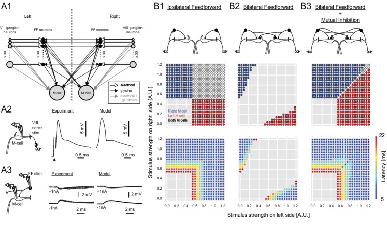
Figure 2. Output of a computational model of the studied neurons in the Mauthner network.

(2A1) Connectivity implemented in the model. Gray arrows indicate mixed electrical and excitatory glutamatergic connections. White arrows indicate pure electrical connections. Black arrows indicate inhibitory glycinergic connections. (2A2) Mauthner response to eighth nerve stimulation. The eighth nerve on one side was stimulated (left panel) and the EPSP in the lateral dendrite of Mauthner cell was recorded experimentally (middle panel). The EPSP in the model was simulated by synchronous activation of eighth ganglion neurons (right panel). (2A3) Inhibitory input from an FF neuron to a Mauthner cell. A single actual FF neuron is activated by current injection to fire a single spike while monitoring IPSPs in the ipsilateral Mauthner cell (left panel). Four traces are shown at potentials above and below reversal potential by injection of plus or minus 1 nA of current into the M-cells (middle panel). The modeled IPSP in the ipsilateral Mauthner cell during injection of plus or minus 1 nA of current (right panel). (2B1) Output of the computational model of Mauthner circuit with only ipsilateral feedforward inhibitory connections (upper panel). Various combinations of left (x-axis) and right stimuli (y-axis) are presented to the model circuit and each stimulus condition is color-coded based on the activation of Mauthner cells (blue: only right Mauthner cell fires, red: only left Mauthner cell fires, white: both Mauthner cells fire) (middle panel) and also based on the latency of the activation (lower panel). (2B2) Output as in B1, but with the addition of asymmetric bilateral feedforward inhibitory connections (upper panel). Middle and lower panels were formatted as in B1. (2B3) Output as in B2, but with the addition of putative reciprocal inhibitory connections between the FF neurons (upper panel).

DOI: http://dx.doi.org/10.7554/eLife.16808.004

Figure 2—figure supplement 1. Outcomes of all of the circuit configurations modeled.

The layout is the same as in Figure 2, with panels A, C and E duplicated from Figure 2 to allow comparison with other variants of the circuit. (B) A circuit like that in C with ipsilateral and contralateral inhibition of the M-cells, but with symmetrical crossed inhibition of the M-cells, instead of the biased crossed inhibition in C that we actually observed experimentally. The symmetrical inhibition of the M-cells in network B leads to a smaller, though still substantial, zone of no escape responses than a similar model with biased inhibition (C). (D–E) Models like those in B and C, but including mutual inhibition between the inhibitory interneurons on opposite sides. Adding mutual inhibition between the inhibitory neurons in each of these recovers escape responses to strong bilateral inputs. This, however, leads to a seemingly more adaptive outcome when the M-cell inhibition is contralaterally biased (E), as this narrows the zone in which both M-cells are simultaneously activated. This configuration matches what we observed experimentally. F and G show model performance when there is only contralateral M-cell inhibition at symmetrical weak or strong levels (the levels are those used for the weak or strong biased connections in other panels, which are based on experiment). Both perform poorly, with large zones of simultaneous or no responses.

DOI: http://dx.doi.org/10.7554/eLife.16808.005