Influence of fat on liver T ₁ measurements using modified Look–Locker inversion recovery (MOLLI) methods at 3T

Abstract

Purpose

To characterize the effect of fat on modified Look–Locker inversion recovery (MOLLI) T ₁ maps of the liver. The balanced steady‐state free precession (bSSFP) sequence causes water and fat signals to have opposite phase when repetition time (TR) = 2.3 msec at 3T. In voxels that contain both fat and water, the MOLLI T ₁ measurement is influenced by the choice of TR.

Materials and Methods

MOLLI T ₁ measurements of the liver were simulated using the Bloch equations while varying the hepatic lipid content (HLC). Phantom scans were performed on margarine phantoms, using both MOLLI and spin echo inversion recovery sequences. MOLLI T ₁ at 3T and HLC were determined in patients (n = 8) before and after bariatric surgery.

Results

At 3T, with HLC in the 0–35% range, higher fat fraction values lead to longer MOLLI T ₁ values when TR = 2.3 msec. Patients were found to have higher MOLLI T ₁ at elevated HLC (T ₁ = 929 ± 97 msec) than at low HLC (T ₁ = 870 ± 44 msec).

Conclusion

At 3T, MOLLI T ₁ values are affected by HLC, substantially changing MOLLI T ₁ in a clinically relevant range of fat content. J. Magn. Reson. Imaging 2016;44:105–111.

THE MODIFIED LOOK–LOCKER INVERSION RECOVERY (MOLLI)1 T ₁ mapping technique and variants of it have been gaining interest in cardiovascular magnetic resonance imaging (MRI)2 and in liver imaging.3 MOLLI is able to build a T ₁ map within a breath‐hold. It has also been demonstrated that MOLLI T ₁ maps provide diagnostic information in the heart4 and correlate with liver fibrosis and inflammation.3

Fat is known to have a short T ₁, and in regions of visceral fat the MOLLI T ₁ method measures this short T ₁ with high reproducibility.5 Similarly, the MOLLI T ₁ method detects long T ₁ regions of the blood pool with high reproducibility.6 Patients suffering from liver‐related diseases have been shown to have fat values in the 2% to 44% range7, 8, 9; thus, in livers with large amounts of fat, simplified reasoning would predict that the measured T ₁ would be the weighted sum of the T ₁ of the fat and the T ₁ of the hepatic tissue. The measured T ₁ of the liver would thus be expected to be reduced in fatty liver due to this partial volume effect. Phantom scans and previous work have demonstrated that T ₁ decreases with increasing fat concentration when using conventional imaging methods, ie, spin echo inversion recovery (SE‐IR).10

MOLLI T ₁ values have been shown to be influenced by fat and off‐resonance frequencies at 1.5T in the calf muscle11 and the myocardium12 and elevated MOLLI T ₁ is often measured in patients with fatty livers3 at 3T, where balanced steady‐state free precession (bSSFP) repetition times (TRs) between 2.1 msec and 2.6 msec are commonly used.3, 13 It is the T ₁ of the water component which appears to be of diagnostic significance when using T ₁ mapping in the liver,14 while the T ₁ of the fat is constant15 and not a predictor of disease. An important step towards the use of MOLLI T ₁ to assess liver disease is the clarification and quantification of the extent to which the presence of fat can mask or exaggerate changes in MOLLI T ₁ due to disease.

The aim of this study was thus to investigate the effect of different fat concentrations and off‐resonance frequencies on MOLLI T ₁ maps at 3T with a bSSFP TR = 2.3 msec and to explain the mechanisms for this behavior.

Theory

MOLLI is an electrocardiogram (ECG)‐gated inversion recovery T ₁ mapping method. It uses several inversion pulses and acquires images synchronized to the cardiac cycle using a snapshot bSSFP16 readout. Readouts are followed by pauses of a few heartbeats, allowing for full recovery of the longitudinal magnetization.1

The bSSFP readout results in images that are sensitive to the off‐resonance frequency of the protons being imaged (Fig. 1).17 The chemical shift difference between water and the main fat peak is 3.5 ppm,18 which at 3T translates into a frequency difference of ∼447 Hz. Therefore, if bSSFP images are acquired with a repetition time close to 1/447 seconds (∼2.23 msec), the fat and water signals will have exactly opposite phase. When a different TR is chosen, the phase relationship between water and fat is a more complex function of off‐resonance frequency.

Figure 1.

Variation of the steady‐state signal over off‐resonance frequencies relative to the water, as seen in Refs. 17 and 34. When a TR equal to the inverse of the chemical shift difference between water and fat is used, the steady‐state signal of fat and water will have opposite phases.

The signal in a voxel containing both fat and water with no exchange of magnetization between them would be determined by the well‐known partial volume effect. If the fat and water were in phase then the recovery would follow the sum of these two recovering exponentials; in practice, if this were fit to a single exponential then the measured T ₁ would lie somewhere between the individual T ₁s of the fat and the water. However, in the situation described in this work the water and fat are exactly out of phase, and so the signal recovery is the difference of two exponentials weighted by the relative contributions of fat and water. In practice, for relatively small fat concentrations this results in a measured value for T ₁ that is longer than the T ₁ value of either the fat or water component.19 A conceptual schematic of this behavior is illustrated in Fig. 2.

Figure 2.

Schematic MOLLI recovery curves of water and fat components at identical main static field strength using TR = 2.3 msec. The 100% fat curve appears inverted because of its frequency shift. The different T ₁ recovery times of fat and water and their opposing phases at TR = 2.3 msec lead to an apparent lengthening of the T ₁ recovery in the combined signal.

Materials and Methods

Simulations

A Bloch equation20 simulation was built in MatLab (MathWorks, Natick, MA) which emulated the exact pulse sequence of a MOLLI acquisition on our scanner. The simulated sequence included the waveforms of radiofrequency (RF) inversion, preparation, and imaging pulses. The measured signal intensity for each simulation was determined as the signal averaged over a set of phase encode lines centered on k = 25. Magnetization transfer effects were not included in the simulation, although they are known to bias T ₁ with the MOLLI method.21

A single inversion followed by five image readouts was simulated, providing a good approximation to the MOLLI acquisition but eliminating the complexity that is due to the multitude of possible sampling schemes that have been described.21 Since liver MOLLI T ₁ values lie in the 700–1400 msec interval,3 five samples over the recovery curve were used for determining the T ₁.

The following simulation parameters were used: 3T field strength, 192 × 144 matrix, 84 phase encode lines, 24 phase encode lines before the central line, flip angle (FA) = 35°, TR/TE = 2.3/1.15 msec, TI = 100, 1000, 1900, 2800, 3700 msec, adiabatic hyperbolic secant 1 inversion pulse of 10.24 msec duration, time‐bandwidth product of R = 5.48, peak B₁ = 750 Hz and β = 3.45.21 The bSSFP readout used five linearly increasing startup angle (LISA) pulses22, 23 and one half‐angle ramp down pulse.

T ₁ and T ₂ values for fat and liver components were: T _1fat = 382 msec, T _2fat = 68 msec,24 T _1hepatic = 812 msec,25 T _2hepatic = 34 msec.24 Separate signals corresponding to each component of a multiple‐peak lipid spectrum were weighted by their relative amplitude provided by Hamilton et al26 and summed to obtain a single fat signal. Simulated fat and water signals were combined in different proportions according to the principle of partial volumes and to reflect HLCs in the 0–100% range in steps of 1%, fat fractions, F, being defined using Eq. (1), where ρ_f and ρ_w denote the proton densities of fat and water.

$$F=\frac{{\rho }_f}{{\rho }_f+{\rho }_w}\times 100[\%]$$ (1)

Then, the signal points were fitted to an exponential describing longitudinal recovery, given by Eq. (2), where T ₁* is the apparent T ₁ and A and B are additional fit parameters.

$$S(TI)=A-B\text{exp}\left(-\frac{TI}{T_1^{*}}\right)$$ (2)

The MOLLI T ₁ values were computed by using the imperfect,27 but commonly used, Look–Locker correction method described by Eq. (3).1

$$T1=T_1^{*}\left(\frac{B}{A}-1\right)$$ (3)

In order to show the changes in MOLLI T ₁ caused by repetition times other than 2.3 msec, the variation of MOLLI T ₁ with off‐resonance frequency was simulated for two repetition times found in the literature: TR = 2.14 msec³ and TR = 2.6 msec.13 All simulation parameters were the same as described above for the liver simulation, with the simplification that only three lipid concentrations were simulated: 0%, 10%, and 20%. The chosen off‐resonance frequency range was –100 Hz to 100 Hz in steps of 2 Hz, which covers the typical frequency range encountered in the in vivo MOLLI data discussed below.

To further explore the effects of fat on MOLLI T ₁ values, the TR was varied in a simulation comprising a water and a multiple‐peak fat component with 30% fat fraction. The spectral model of the fat was based on the ¹H spectrum of the margarine phantom described below. The same imaging protocol was simulated as described in the previous section, with the following differences: TI = 200, 1200, 2200, 3200, 4200 msec, RR = 1000 msec, and 31 bSSFP TR values in the range 1.93 to 5.75 msec. T ₁ and T ₂ values for fat and water components corresponded to those of a margarine phantom and were T _1fat = 325 msec, T _2fat = 120 msec, T _1water = 2448 msec, and T _2water = 207 msec. The measurements leading to these values are described in the next section.

Phantom Scans

Phantom experiments were carried out using a margarine phantom (Flora Light, Unilever) with 30% fat content. First, the margarine phantom was scanned using a 5‐point MOLLI sequence. Imaging parameters followed a standardized MOLLI acquisition protocol (Siemens WIP 561a, Erlangen, Germany): 192 × 144 matrix, FA = 35°, TR/TE = 2.3/0.99 msec, TI = 100, 1100, 2100, 3100, 4100 msec, simulated ECG with RR = 1000 msec. Then the same margarine phantom was scanned using the SE‐IR sequence. Imaging parameters followed a standardized acquisition protocol: 128 × 128 matrix, TR = 10000 msec, TI = 50, 150, 250, 400, 600, 900, 1300, 2000, 3000, 4500, 6500 msec, TE = 7.4 msec. In both cases images were acquired using a Siemens 3T Verio scanner using a 32‐channel head RF coil.

Following the margarine scans, a sample of the margarine was heated and then spun with a centrifuge (Rotanta 460R, Hettich) at 4000 rpm for 5 minutes. After spinning the sample, separate layers of fat and water were obtained that were scanned using the MOLLI acquisition and the SE‐IR acquisition using the same scanner and same protocols as described above.

A subsequent experiment was carried out in order to determine MOLLI T ₁ of the whole margarine and the water component only over a range of repetition times. The previously described 5‐point MOLLI acquisition protocol was used with the following changes: TI = 200, 1200, 2200, 3200, 4200 msec, RR = 1000 msec, and 31 bSSFP TR values ranging from 1.93 to 5.75 msec.

MOLLI T ₁ values were determined by fitting the signal intensity of a circular region of interest on the bSSFP images following the inversion pulse to Eq. (2), then applying Eq. (3) to obtain T ₁. T ₁ values for images acquired using the SE‐IR sequence were computed by fitting Eq. (4) to mean signal values sampled from the same region of interest in each image.

$$S(TI)=C\left(1-2\text{exp}\left(-\frac{TI}{T_1}\right)+\text{exp}\left(-\frac{TR}{T_1}\right)\right)$$ (4)

Patient Studies

In order to compare the results of the simulations to results obtained in vivo, data from eight patients (seven female, mean age: 49 ± 10.5 years) were processed retrospectively. Patients were scanned before weight reduction surgery and 6 months postoperatively. Relevant parameters of the patients before surgery included mean body mass index (BMI): 45.8 ± 5.5 kg/m², mean waist circumference: 120.25 ± 10.35 cm, and mean hip circumference: 134.5 ± 11.2 cm. Four of the patients suffered from diabetes. Postoperative parameters were: mean BMI: 36.4 ± 4.8 kg/m², mean waist circumference: 107.7 ± 10.6 cm, and mean hip circumference: 120.6 ± 8.6 cm.

The study protocol conformed to the ethical guidelines of the 1975 Declaration of Helsinki, and was approved by the institutional research departments and the National Research Ethics Service (13/SC/0243). All patients gave written informed consent.

At each timepoint, patients had liver MOLLI T ₁ maps (5‐point MOLLI was employed). T ₂* maps were collected for hepatic iron quantification and ¹H MRS for the quantification of liver fat using the stimulated echo acquisition mode (STEAM) sequence. Imaging parameters for the MOLLI scan were: 192 × 134–160 matrix (depending on patient), field of view (FOV) 280–348 × 350–500 mm (depending on patient), slice thickness of 8 mm, GRAPPA acceleration factor 2, pixel bandwidth 898 Hz/px, TR/TE = 2.14/1.07 msec, FA = 35°, TI = 110, 110+RR, 110+2RR, 110+3RR, 110+4RR msec. MOLLI T ₁ maps were acquired in transverse scan planes.

T ₂* maps were determined using a multiecho acquisition with RF spoiling. Imaging parameters for this acquisition were as follows: same FOV as for the 5‐point MOLLI sequence, 192 × 128–160 matrix (depending on patient), slice thickness of 3 mm, GRAPPA acceleration factor 2, TR/TE = 26.5/2.46, 7.38, 12.30, 17.22, 22.14 msec, FA = 20°. Fat saturation and double‐inversion black blood preparation were used.

The STEAM spectroscopy experiment used28: TE = 10 msec, TM = 7 msec, TR = 2 seconds for water‐suppressed spectra and TR = 4 seconds for water‐unsuppressed spectra and voxel volume was 8 cm³. The voxel of interest was placed in the lateral part of the right lobe of the liver, avoiding vessels, bile ducts, and the edge of the liver. Spectra were processed using AMARES in jMRUI29 with a specialized MatLab script28 and the fat fraction was determined as the ratio of the fat signal and the sum of the fat and water signals as in Eq. (1).

Results

Simulation

Figure 3 presents the relationship between the simulated MOLLI T ₁ and HLC. At low HLC (0–16% range) the measured MOLLI T ₁ increases with increasing fat, and can be approximated by:

$$MOLLI\hspace{0.5em}{T}_1=715+5.47F+0.27F^2$$ (5)

where MOLLI T ₁ is expressed in milliseconds and F is the percent HLC. This trend ends at approximately F = 40%, where fitting becomes impossible owing to the water signal and fat signal canceling each other out. For F > 50% the MOLLI T ₁ values change rapidly, eventually reaching the T ₁ of the fat at 100% fat fraction. The increase of MOLLI T ₁ is explained by the simultaneous increase of both the B/A ratio and the apparent T ₁ (T ₁*) in Eq. (3).

Figure 3.

Variation of simulated MOLLI T ₁ values of the liver with fat fraction emphasizing behavior at off‐resonance: (a) global behavior of MOLLI T ₁ values over the full range of fat fractions; (b) MOLLI T ₁ behavior corresponding to the 0–16% range of fat fractions.

Figure 3 also presents the behavior of MOLLI T ₁ variation in the case of off‐resonance. Although the bSSFP readout leads to a symmetric MOLLI T ₁ variation around the central water frequency for 0% HLC, using a multiple‐peak spectral model of the lipid leads to asymmetric off‐resonance frequency dependence.

In simulations the dependence of MOLLI T ₁ on off‐resonance frequency when using repetition times from the literature3, 13 is shown in Fig. 4. Simulated MOLLI T ₁ values were found to be higher at lower repetition times for most fat fractions and off‐resonance frequencies. In addition, MOLLI T ₁–off‐resonance frequency dependence is both larger and increasingly asymmetric with respect to frequency in the presence of higher fat.

Figure 4.

Variation of simulated MOLLI T ₁ with off‐resonance frequency and using repetition times described in the literature.3, 13

Phantom Scans

T ₁ values determined from MOLLI and SE‐IR experiments in the margarine phantom are presented in Table 1.

Table 1.

T₁ Values Measured by the MOLLI Method and Computed From SE‐IR Images

	30% margarine
Phantom type	MOLLI T1 [msec]	SE‐IR T1 [msec]
Whole margarine	3874 ± 177	1313 ± 14
Fat component	291 ± 23	325 ± 20
Water component	2266 ± 21	2448 ± 7

Figure 5 shows the signal intensities taken from regions of interest on SE‐IR images and the curves fitted to these points, along with the signal intensities sampled from MOLLI acquisitions and corresponding fitted curves.

Figure 5.

Fitted T ₁ recovery curves of whole margarine, fat component, and water component in the 30% fat margarine phantom: (a) shows the results of the spin echo inversion recovery experiment; (b) shows the results of the MOLLI experiment.

The results of the simulation and phantom experiment exploring the dependence of MOLLI T ₁ on repetition times is shown in Fig. 6. Both simulated and measured MOLLI T ₁ values of the margarine phantom with 30% fat were higher than those of water over the 1.8 to 3.5 msec range and lower over the 3.5 to 5.75 msec range due to the relative position of the bSSFP profiles of the fat and water. However, the simulated and measured data did not agree perfectly. A possible explanation for the mismatch could be the missing information on the different T ₁ and T ₂ values of the individual fat peaks in the margarine phantom. A similar difference between simulation and phantom experiments can be seen in Thiesson et al's work.11

Figure 6.

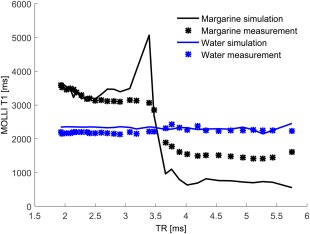
Variation of MOLLI T ₁ with the change of TR. Fat and water are out of phase at TR = 2.3 msec and in phase at TR = 4.6 msec.

Patient Studies

One patient was excluded from the comparison because the T ₁ fit to the MOLLI data failed at the first visit. The measured HLC for this patient was 39.7%, which is in the regime where the Bloch simulated data could also not be fitted to an inversion recovery model.

Six patients had normal T ₂* values larger than 19 msec and one had T ₂* = 15 msec, indicating elevated iron but all within the normal range for T ₂* at 3T.30

Pre‐ and postoperative MOLLI T ₁ measurements for seven patients are shown in Fig. 7, plotted as a function of their spectroscopically measured HLC. Simulated relationships between T ₁ and HLC are also included for three different levels of liver fibrosis, characterized by the Ishak score.31 MOLLI T ₁ values at 0% HLC for the three curves were taken from Banerjee et al, as shown in their fig. 2 of Ref. 3. The changes in MOLLI T ₁ that occur in these patients are consistent with the hypothesis that the water in the livers of these patients is elevated but stable between exams and that the fat concentration has changed. These patients are expected to have some level of inflammation or fibrosis, which has previously been shown to elevate MOLLI T ₁.3

Figure 7.

Continuous lines represent the variation of simulated MOLLI T ₁ with HLC, for three levels of liver fibrosis as defined by the Ishak score. These curves were obtained by running the simulation for T ₁ values corresponding to different disease states as described by Banerjee et al3 (see their fig. 2). Dashed line segments connect patient data points, showing the change in measured MOLLI T ₁ for each individual.

Discussion

In a physiological range of HLC from 0% to 45%7, 8, 9 we have shown that the MOLLI T ₁ at 3T increases with fat concentration in simulation and phantoms when using TR = 2.3 msec. This also applies when TR lies in the range 2.1 to 2.6 msec. The MOLLI T ₁ elevation is seen in vivo with the caveat that there may be other changes in the livers of the patients over 6 months after bariatric surgery that would be expected to modify the T ₁.3

Due to a chemical shift difference of 447 Hz between fat and water at 3T, the two tissue components are exactly out of phase with their passbands overlapping when using TR = 2.3 msec. Thus, combined signals from tissue containing fat and water are less dependent on off‐resonance frequency than reported previously using TR = 2.7 msec at 1.5T.11 Increasing or decreasing the TR from 2.3 msec at 3T reduces the overlap of the two bSSFP passbands, increasing the off‐resonance frequency dependence.

These simulations suggest that careful shimming, in addition to the use of a TR of 2.3 msec or less, is useful to maximize the consistency of MOLLI T ₁ measurements within a single subject and between subjects.

In contrast to 3T, where the optimal TR for reducing the frequency dependence of MOLLI T ₁ measurements is close to the minimum TR available with existing hardware, at 1.5T longer TR values would have to be used to produce a similar overlapping of the two bSSFP passbands due to the smaller chemical shift difference between fat and water.32

Patient MOLLI T ₁ evolution in a 6‐month interval after bariatric surgery follows our model describing the influence of fat on MOLLI T ₁ values. We expect that, while the amount of fat changes in these patients, other parameters known to affect the T ₁ (such as fibrosis and inflammation) remain fairly constant. In general terms, the change in measured MOLLI T ₁ is consistent with the behavior that is predicted by the simulation for changes in liver fat in five of the seven patients; in one patient the change in liver fat is very small and the MOLLI T ₁ change is small, and in one patient the liver fat change is small, but the MOLLI T ₁ change is ∼100 msec, not following the model. We believe that this supports the applicability of the model in vivo.

A limitation of this study is the small size of the patient cohort. A change in MOLLI T ₁ in two of the patients was not explained by change in fat fractions, suggesting the existence of other mechanisms responsible for having an influence on hepatic MOLLI T ₁ values.

The MOLLI T ₁ mapping method is used extensively in cardiac imaging and so it is important to briefly consider the effect of myocardial fat on MOLLI T ₁ maps at 3T. Since global lipid fractions in the myocardium are in the 0.2–2% interval,28, 33 they have a much smaller effect on measured MOLLI T ₁ values. An exception is in focal lipid accumulations, which can be as high as 35% in the case of lipomatous metaplasia,12 leading to replacement of scar tissue with lipid accumulations after myocardial infarction. Effects of these focal lipid concentrations are described by Kellman et al.12

In conclusion, this study has shown that the presence of fat influences MOLLI T ₁ measurements in the liver. This effect is in addition to the previously known effects of T ₂, magnetization transfer, off‐resonance frequency, and iron concentration. Simulation has shown that fat fractions up to 40% will have an additive effect on the measured MOLLI T ₁ value at 3T when using a bSSFP readout with TR = 2.3 msec. This behavior has been confirmed in the livers of patients undergoing weight‐reduction surgery.

The influence of fat should be considered in the assessment of hepatic diseases using MOLLI T ₁ measurements, as fat fraction values measured in the liver can be large enough to cause severe MOLLI T ₁ alterations.

References

- 1. Messroghli DR, Radjenovic A, Kozerke S, Higgins DM, Sivananthan MU, Ridgway JP. Modified Look‐Locker inversion recovery (MOLLI) for high‐resolution T1 mapping of the heart. Magn Reson Med 2004;52:141–146. [DOI] [PubMed] [Google Scholar]
- 2. Moon JC, Messroghli DR, Kellman P, et al. Myocardial T1 mapping and extracellular volume quantification: a Society for Cardiovascular Magnetic Resonance (SCMR) and CMR Working Group of the European Society of Cardiology consensus statement. J Cardiovasc Magn Reson 2013;15:92. [DOI] [PMC free article] [PubMed] [Google Scholar]
- 3. Banerjee R, Pavlides M, Tunnicliffe EM, et al. Multiparametric magnetic resonance for the non‐invasive diagnosis of liver disease. J Hepatol 2014;60:69–77. [DOI] [PMC free article] [PubMed] [Google Scholar]
- 4. Ferreira VM, Piechnik SK, Robson MD, Neubauer S, Karamitsos TD. Myocardial tissue characterization by magnetic resonance imaging: novel applications of T1 and T2 mapping. J Thorac Imaging 2014;29:147–154. [DOI] [PMC free article] [PubMed] [Google Scholar]
- 5. Ferreira VM, Holloway CJ, Piechnik SK, Karamitsos TD, Neubauer S. Is it really fat? Ask a T1‐map. Eur Heart J Cardiovasc Imaging 2013;14:1060. [DOI] [PMC free article] [PubMed] [Google Scholar]
- 6. Vassiliou V, Heng EL, Sharma P, et al. Reproducibility of T1 mapping 11‐heart beat MOLLI Sequence. J Cardiovasc Magn Reson 2015;17(Suppl 1):W26. [Google Scholar]
- 7. Bannas P, Kramer H, Hernando D, et al. Quantitative magnetic resonance imaging of hepatic steatosis: validation in ex vivo human livers. Hepatology 2015;62:1444–1455. [DOI] [PMC free article] [PubMed] [Google Scholar]
- 8. Tang A, Tan J, Sun M, et al. Nonalcoholic fatty liver disease: MR imaging of liver proton density fat fraction to assess hepatic steatosis. Radiology 2013;267:422–431. [DOI] [PMC free article] [PubMed] [Google Scholar]
- 9. Idilman IS, Aniktar H, Idilman R, et al. Hepatic steatosis: quantification by proton density fat fraction with MR imaging versus liver biopsy. Radiology 2013;267:767–775. [DOI] [PubMed] [Google Scholar]
- 10. Rakow‐Penner R, Daniel B, Yu H, Sawyer‐Glover A, Glover GH. Relaxation times of breast tissue at 1.5T and 3T measured using IDEAL. J Magn Reson Imaging 2006;23:87–91. [DOI] [PubMed] [Google Scholar]
- 11. Thiesson S, Thompson R, Chow K. Characterization of T1 bias from lipids in MOLLI and SASHA pulse sequences. J Cardiovasc Magn Reson 2015;17(Suppl 1):W10. [DOI] [PubMed] [Google Scholar]
- 12. Kellman P, Bandettini WP, Mancini C, Hammer‐Hansen S, Hansen MS, Arai AE. Characterization of myocardial T1‐mapping bias caused by intramyocardial fat in inversion recovery and saturation recovery techniques. J Cardiovasc Magn Reson 2015;17:33. [DOI] [PMC free article] [PubMed] [Google Scholar]
- 13. de Meester de Ravenstein C, Bouzin C, Lazam S, et al. Histological validation of measurement of diffuse interstitial myocardial fibrosis by myocardial extravascular volume fraction from modified Look‐Locker imaging (MOLLI) T1 mapping at 3 T. J Cardiovasc Magn Reson 2015;17:48. [DOI] [PMC free article] [PubMed] [Google Scholar]
- 14. Leporq B, Ratiney H, Pilleul F, Beuf O. Liver fat volume fraction quantification with fat and water T1 and T2* estimation and accounting for NMR multiple components in patients with chronic liver disease at 1.5 and 3.0 T. Eur Radiol 2013;23:2175–2186. [DOI] [PubMed] [Google Scholar]
- 15. Hamilton G, Middleton MS, Hooker JC, et al. In vivo breath‐hold (1) H MRS simultaneous estimation of liver proton density fat fraction, and T1 and T2 of water and fat, with a multi‐TR, multi‐TE sequence. J Magn Reson Imaging 2015;42:1538–1543. [DOI] [PMC free article] [PubMed] [Google Scholar]
- 16. Bieri O, Scheffler K. Fundamentals of balanced steady state free precession MRI. J Magn Reson Imaging 2013;38:2–11. [DOI] [PubMed] [Google Scholar]
- 17. Scheffler K, Lehnhardt S. Principles and applications of balanced SSFP techniques. Eur Radiol 2003;13:2409–2418. [DOI] [PubMed] [Google Scholar]
- 18. Yu H, McKenzie CA, Shimakawa A, et al. Multiecho reconstruction for simultaneous water‐fat decomposition and T2* estimation. J Magn Reson Imaging 2007;26:1153–1161. [DOI] [PubMed] [Google Scholar]
- 19. Kellman P, Wilson JR, Xue H, Ugander M, Arai AE. Extracellular volume fraction mapping in the myocardium. Part 1: Evaluation of an automated method. J Cardiovasc Magn Reson 2012;14:63. [DOI] [PMC free article] [PubMed] [Google Scholar]
- 20. Brown RW, Cheng Y‐CN, Haacke EM, Thompson MR, Venkatesan R. (eds.). Magnetization, relaxation, and the Bloch equation In: Magnetic resonance imaging: physical principles and sequence design, 2nd ed Hoboken, NJ: John Wiley & Sons; 2014. p 53–66. [Google Scholar]
- 21. Robson MD, Piechnik SK, Tunnicliffe EM, Neubauer S. T1 measurements in the human myocardium: The effects of magnetization transfer on the SASHA and MOLLI sequences. Magn Reson Med 2013;70:664–670. [DOI] [PubMed] [Google Scholar]
- 22. Nishimura DG, Vasanawala SS. Analysis and Reduction of the Transient Response in SSFP Imaging. In: Proc 8th Annual Meeting ISMRM, Denver; 2000:301.
- 23. Deshpande VS, Shea SM, Laub G, Simonetti OP, Finn JP, Li D. 3D magnetization‐prepared true‐FISP: a new technique for imaging coronary arteries. Magn Reson Med 2001;46:494–502. [DOI] [PubMed] [Google Scholar]
- 24. de Bazelaire CMJ, Duhamel GD, Rofsky NM, Alsop DC. MR imaging relaxation times of abdominal and pelvic tissues measured in vivo at 3.0 T: preliminary results. Radiology 2004;230:652–659. [DOI] [PubMed] [Google Scholar]
- 25. Stanisz GJ, Odrobina EE, Pun J, et al. T1, T2 relaxation and magnetization transfer in tissue at 3T. Magn Reson Med 2005;54:507–512. [DOI] [PubMed] [Google Scholar]
- 26. Hamilton G, Yokoo T, Bydder M, et al. In vivo characterization of the liver fat 1H MR spectrum. NMR Biomed 2011;24:784–790. [DOI] [PMC free article] [PubMed] [Google Scholar]
- 27. Deichmann R, Haase A. Quantification of T1 values by SNAPSHOT‐FLASH NMR imaging. J Magn Reson 1992;96:608–612. [Google Scholar]
- 28. Rial B, Robson MD, Neubauer S, Schneider JE. Rapid quantification of myocardial lipid content in humans using single breath‐hold 1H MRS at 3 Tesla. Magn Reson Med 2011;66:619–624. [DOI] [PMC free article] [PubMed] [Google Scholar]
- 29. Naressi A, Couturier C, Devos JM, et al. Java‐based graphical user interface for the MRUI quantitation package. Magma Magn Reson Mater Phys Biol Med 2001;12:141–152. [DOI] [PubMed] [Google Scholar]
- 30. Storey P, Thompson AA, Carqueville CL, Wood JC, de Freitas RA, Rigsby CK. R2* imaging of transfusional iron burden at 3T and comparison with 1.5T. J Magn Reson Imaging 2007;25:540–547. [DOI] [PMC free article] [PubMed] [Google Scholar]
- 31. Ishak K, Baptista A, Bianchi L, et al. Histological grading and staging of chronic hepatitis. J Hepatol 1995;22:696–699. [DOI] [PubMed] [Google Scholar]
- 32. Hargreaves BA, Vasanawala SS, Nayak KS, Hu BS, Nishimura DG. Fat‐suppressed steady‐state free precession imaging using phase detection. Magn Reson Med 2003;50:210–213. [DOI] [PubMed] [Google Scholar]
- 33. Liu C‐Y, Bluemke DA, Gerstenblith G, et al. Myocardial steatosis and its association with obesity and regional ventricular dysfunction: evaluated by magnetic resonance tagging and 1H spectroscopy in healthy African Americans. Int J Cardiol 2014;172:381–387. [DOI] [PMC free article] [PubMed] [Google Scholar]
- 34. Bernstein MA. Basic pulse sequences In: Bernstein MA, King KF, Zhou XJ, editors. Handbook of MRI pulse sequences, 1st ed Amsterdam: Elsevier; 2004. p 594. [Google Scholar]