Misclassification Errors in Unsupervised Classification Methods. Comparison Based on the Simulation of Targeted Proteomics Data

Abstract

Unsupervised classification methods are gaining acceptance in omics studies of complex common diseases, which are often vaguely defined and are likely the collections of disease subtypes. Unsupervised classification based on the molecular signatures identified in omics studies have the potential to reflect molecular mechanisms of the subtypes of the disease and to lead to more targeted and successful interventions for the identified subtypes. Multiple classification algorithms exist but none is ideal for all types of data. Importantly, there are no established methods to estimate sample size in unsupervised classification (unlike power analysis in hypothesis testing). Therefore, we developed a simulation approach allowing comparison of misclassification errors and estimating the required sample size for a given effect size, number, and correlation matrix of the differentially abundant proteins in targeted proteomics studies. All the experiments were performed in silico. The simulated data imitated the expected one from the study of the plasma of patients with lower urinary tract dysfunction with the aptamer proteomics assay Somascan (SomaLogic Inc, Boulder, CO), which targeted 1129 proteins, including 330 involved in inflammation, 180 in stress response, 80 in aging, etc. Three popular clustering methods (hierarchical, k-means, and k-medoids) were compared. K-means clustering performed much better for the simulated data than the other two methods and enabled classification with misclassification error below 5% in the simulated cohort of 100 patients based on the molecular signatures of 40 differentially abundant proteins (effect size 1.5) from among the 1129-protein panel.

Introduction

Some complex common diseases are vaguely defined and are more properly referred to as syndromes, i.e., sets of medical signs and symptoms without a defined or distinct etiology. Many of these common diseases are likely a collection of disease subtypes that require different diagnostics and treatments [1,2]. Lower urinary tract dysfunction (LUTD) is a good example.

The presence and severity of urinary symptoms is largely subjective and may be the result of a multitude of pathological processes [3]. Therefore, classification based solely on the predominant symptoms may be unsatisfactory and needs to be complemented by unbiased (objective) classification based on molecular signatures, i.e., groups of the differentially abundant proteins. Classification based on biomarker signatures rather than clinical symptoms is expected to reflect molecular mechanisms of the subtypes of the disease and to lead to more targeted and successful interventions. The initial goal of this study was very practical: to estimate the required sample size (number of patients) and to choose an algorithm for the unsupervised classification of patients in a biomarker study that is part of the large NIH-funded collaborative study Symptoms of Lower Urinary Tract Dysfunction Research Network (LURN). There are no established methods to estimate sample size in unsupervised classification (unlike power analysis in hypothesis testing). Therefore, we developed an approach to estimate misclassification error given an expected number of differentially abundant proteins, number of disease subtypes, effect size, and number of patients in the study. An appropriate sample size would give a low misclassification error, such as 5%, for a desired effect size for over a reasonable range of other parameters.

Many unsupervised classification methods exist [4] including k-means clustering, fuzzy k-means clustering, hierarchical clustering, principal component analysis (PCA), nonlinear component analysis, independent component analysis, multidimensional scaling, and self-organizing maps. Recently, this group of methods was complemented by an even more sensitive classification technique called topological data analysis [5], which proved to be useful in a broad range of multidimensional data analysis applications ranging from detection of subtypes of breast cancer [6] to exploring the states of folding pathways of biopolymers [7], and even classification of the voting patterns of the members of the US House of Representatives [8]. However, none of the classification methods is ideal in all settings and the optimal choice of the method depends on the properties of the underlying data. Comparison of the performance of the unsupervised algorithms is not straightforward when analyzing real data with unknown class membership (unlabeled data). Several criteria need to be considered when comparing algorithms, including: ratio of the between-cluster variance and within-cluster variance, robustness of classification to the removal of random members of the population, robustness to missing data. The situation is much simpler in the case of simulated data, where true class membership is determined a priori and the misclassification error, i.e., ratio of the number of objects wrongly classified to the total number of objects in the dataset, can be easily calculated.

A recent review of the multivariate statistical methods used in proteomics [9] demonstrated that the most popular unsupervised classification methods in proteomics studies were PCA and hierarchical clustering, which were used in 19 and 7, respectively, out of 26 reviewed proteomics papers (see Table 2 of reference [9]). Strictly speaking, PCA is not a classification method, but a method to visualize multidimensional data by projecting it on new axes - principal components, i.e., the orthogonal uncorrelated linear combinations of the original variables, where the first and each of the following orthogonal principal components account for as much of the variability in the data as possible. Most proteomics papers using PCA present cases where the separation of the groups is visible in scatter plots of one component versus another; however, the degree of separation is not quantified and therefore the results remain qualitative and difficult to assess, especially when the separation is far from perfect.

In this paper, we compare three commonly used clustering methods: hierarchical, k- means, and k-medoids, which unlike PCA provide quantitative results for class memberships, and therefore allow comparison even in the case of poor separation. We illustrate our method for the case of targeted proteomics studies, where all of the measured proteins are known to be relevant to disease pathways and the missing data is much less prevalent than in the case of shotgun proteomics. As an example, we simulated the data that we expect from the study of plasma of patients with lower urinary tract dysfunction (LUTD) using the aptamer proteomics assay Somascan (SomaLogic Inc, Boulder, CO), which targets 1129 proteins, including 330 involved in inflammation, 300 in signal transduction, 190 in cardiovascular diseases, 180 in stress response, 80 in aging, 70 in renal diseases, with a few proteins in more than one category. LUTD is known to be related to inflammation, stress, and aging. Therefore, we expect a substantial number of these proteins to be differentially abundant in LUTD subtypes.

It is typical for proteomic studies to demonstrate a large number of differentially abundant proteins in cases versus controls. For example, 44 serum proteins were found significantly differentially abundant in the SomaScan study of 51 patients with Duchenne muscular dystrophy versus 17 age matched controls [10], 248 differentially abundant proteins were observed in the SomaScan study of CSF of patients with age-related neurodegeneration versus controls [11], and 239 significantly differentially abundant proteins were observed in the SomaScan study of serum of 39 patients after 8 weeks of pulmonary tuberculosis treatment relative to the baseline [12]. Similarly in shotgun proteomics, 116 differentially abundant proteins were identified in chronic pancreatitis versus controls [13], synchronous dynamics of abundances over time of about 90 proteins was observed reflecting both short- and long-term effects of leptin-replacement therapy [14] and 197 proteins were shown to be significantly differentially abundant in Alzheimer’s disease versus control brain samples [15]. Recently, classifiers were developed based on the presence of differentially abundant proteins and naturally occurring peptides in urine: a classifier of stroke contained 31 biomarkers [16] and a classifier of chronic kidney disease had 273 biomarkers [17]. Therefore, we expect that the biomarker signatures defining the subtypes of diseases can contain substantial number of differentially abundant proteins involved in up- or down-regulated pathways.

Figure 1 provides the schematic representation of our analysis. Protein abundances were simulated given the number of patients P, number of proteins in the assay N, number of patient clusters K, list of class membership L, number of biomarkers in the signature M, effect size Eff, and correlation matrix of protein abundances R. Then, three clustering algorithms were used to cluster patients in the simulated data (true L unknown to the clustering algorithms). Finally, lists of class memberships predicted by the algorithms were compared with the true class membership L and misclassification error rate was calculated. Input parameters P, N, K, M, Eff as well as structure of correlation matrix and values of correlation coefficients were varied.

Figure 1.

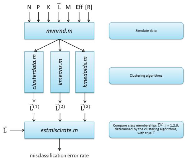
Schematic representation of the analysis. Analysis involves three parts. First, simulate data based on the following inputs: P-number of patients, N-number of proteins in the assay, K- number of patient clusters, L –list of class membership with P elements, where each element Li (i=1,2,…P) is an integer q=1,2,…K. Other inputs are: M – number of differentially abundant proteins (candidate biomarkers), Eff_nq- effect size (could be different for each protein n and each cluster q), R- correlation matrix of protein abundances. Second, use simulated data as an input to the clustering algorithms (in this paper: hierarchical clustering, k-means, and k-medoids). Third, compare lists of class memberships L^(r) r=1,2,3 generated by the clustering algorithms with the true list of class membership L; determine misclassification error rate. Vary inputs, e.g. Eff and P, repeat the whole procedure, create plots of misclassification error vs. Eff. Determine the threshold value of effect size which enables misclassification error below 5% for the given number of patients P, or determine the number of patients (sample size of the future study), which enables misclassification error below 5% for the given expected Eff. See detailed explanation in the text.

Methods

Clustering algorithms

All the simulation experiments were performed in silico. Clustering algorithms were used as implemented in MATLAB 2015a Statistics and Machine Learning Toolbox functions: clusterdata.m, kmeans.m and kmedoids.m. Function evalclusters.m from the same toolbox was used to evaluate quality of clustering by using four criteria: Calinski-Harabasz [18], Davies- Bouldin [19], Gap [20], and Silhoutte [21]. The description of the functions can be found in MATLAB documentation. Briefly, function clusterdata.m performs agglomerative hierarchical cluster analysis on a data set by the following procedure: distance between all data points is calculated, pairs of data points are linked that are in the closest proximity; then, as data points are paired into binary clusters, the newly formed clusters are grouped into larger clusters until a hierarchical tree is formed; finally, decision is made on where to ‘draw the horizontal line’ and cut the hierarchical tree into clusters. Function kmeans.m uses an iterative algorithm that minimizes the sum of distances from each data point to its cluster centroid, over all clusters. This algorithm moves data points between clusters until the sum cannot be decreased further. Similar to k-means, k-medoids is a partitioning method that is used in cases that require robustness to outlier data. Importantly in k-medoids, centroid is always one of the actual data points of the cluster. See more on comparison of hierarchical clustering, k-means and k- medoids in the Results section. Function evalclusters.m implements the above four criteria of cluster quality defined in [18-21] and described in MATLAB documentation. Briefly, Calinski- Harabasz, Davies-Bouldin and Silhoutte compare between cluster variances with within cluster variances and differ by the way these variances are defined. In addition, Calinski-Harabasz criterion penalizes the case where the number of clusters is high and commensurate with the number of data points in the dataset. Gap criterion is more computationally intense since it compares the within cluster dispersion with the expected value of within cluster dispersion for the reference distribution.

Simulated datasets

Simulated datasets were matrices of log-transformed protein abundances: A_ik =log(abundance of the i^th protein in the k^th patient’s sample), where i=1…N and k=1…P. Protein abundances were assumed to be distributed log-normally. A log-normal process is the statistical realization of the multiplicative product of many independent random variables, each of which is positive, which is in line with the observation that distributions of omics measurements are satisfactorily described by log-normal distributions, since multiplicative regulatory mechanisms are causally dominant in biological systems [22]. Importantly, protein abundances might vary in plasma by 9 orders of magnitude, but are obviously always positive, which is better described by the log-normal than by the normal distribution. Protein abundances were assumed to be measured by SomaScan, or by some other targeted (e.g. multiple reaction monitoring) proteomics technique. Therefore, we assumed the absence of missing data, which is typical for targeted proteomics in contrast with shotgun proteomics, where missing data are quite prevalent. Biological variability of the patients as well as possible measurement errors were represented by simulating the logarithms of protein abundances as random numbers with multivariate normal distribution generated with MATLAB function mvnrnd.m. For the reasons explained in the next section, abundances of the proteins were not considered to be independent, and therefore non- diagonal correlation matrices were used in the mvnrnd.m function to represent these dependencies. An example of the simulated dataset is available as a supplementary file.

Correlation of protein abundances

Proteins in the targeted proteomics assays are usually selected to represent some important processes, pathways, or diseases. Some of these proteins can participate in the same pathways and/or can be regulated by the same transcription regulation factors. Abundances of these proteins are not independent and were therefore simulated as correlated variables. We anticipated that the values of the correlation coefficients and the structure of the correlation matrix could affect the ability of the clustering methods to classify data. The limiting case of total/complete correlation R_ij=1, for all i and j (i=1…N, j=1…N are protein indices) is obvious, since it reduces the protein panel to a single biomarker, which is clearly a less powerful classifier than the biomarker panel. To evaluate the effect of the correlation of protein abundances, we examined two types of the correlation matrices. In the first case, we assumed that the protein assay could be simulated as a collection of non-overlapping groups of proteins. Correlation between the pairs of proteins within the group was equal to R; correlation with the proteins outside the group was zero. We call this correlation structure ‘within group’ correlation. In the second case, we assumed that all the proteins in the assay are correlated but to a decreasing extend as the indices are farther apart. We simulated the correlation matrix as R_ij = R∣i-j∣, i.e., R₁₁=1, R₁₂=R₂₁=R, R₁₃=R₃₁=R², etc. For brevity we will call it the ‘among neighbors’ correlation. Clearly, these two cases do not cover all the possible combinatorial complexity of the protein abundance interdependences, but provide the way to compare the effects of various types of correlation on the classification capability of the algorithm.

Biomarker signatures

Following the same spirit of reducing of the combinatorial complexity of possible structures of the biomarker signatures, we simulated the two limiting cases of totally non- overlapping and totally overlapping biomarker signatures of the subtypes of the disease. We assumed that the disease of interest has K subtypes which are present in the population of patients. So the simulated number of clusters was K. In the first case, we assumed that each of the clusters is represented by a signature of M differentially abundant proteins and that this signature does not overlap with the signatures of any other patient clusters, meaning that these M proteins are differentially abundant only in one of the patient clusters, while in the other patient clusters the abundance of these proteins is similar to those of control subjects. In the second case, we assumed that there were only M differentially abundant proteins in the whole protein abundance matrix and that the difference between the signatures of the patient clusters was in the sign of the differential abundance for each particular protein. Therefore, each of the cluster signatures was represented as the M-long sequence of “+” and “−”.

Standardization of proteins abundances

One of the important choices in unsupervised classification is whether to standardize or not to standardize the variables. As described in [23], the problem with unstandardized data is the inconsistency between cluster solutions when the scale of variables is changed, which is a strong argument in favor of standardization. The common form of conversion of the variables to standard scores (or z-scores) entails subtracting the mean and dividing by the standard deviation for each variable (protein). However, standardization defined in this way is not suitable for our task of defining disease subtypes. Subtracting the overall mean and dividing by the overall standard deviation ignoring whether it is caused by the natural biological variability of the patients or by the differences in the disease subtypes would mask the subtype differences. The solution to this problem is standardization by the mean and standard deviation of the control subjects group, who do not have the disease of interest. Following this approach, we defined standardized variables as:

$${\mathit{Z}}_{\mathit{ik}}=(A_{\mathit{ik}}-A_{\mathit{ic}})∕{\sigma }_{\mathit{ic}}$$ (1)

where $A_{\mathit{ic}}$ and σ_ic – mean and standard deviation of the log(abundances) of the i^th protein in the control group. Assuming that the standard deviations of log(abundances) within each disease subtype are similar to the standard deviation within the control group, we can now simulate standardized log(abundances) as normal distributions with standard deviation equal to 1 with mean equal to:

$${\mathit{Eff}}_{\mathit{ij}}={\mathit{z}}_{\mathit{ij}}=({\widehat{A}}_{\mathit{ij}}-A_{\mathit{ic}})∕{\sigma }_{\mathit{ic}}$$ (2)

where ${\widehat{A}}_{\mathit{ij}}$ the average log(abundance) of protein i across all the patients belonging to the cluster (disease subtype) j. By analogy with the usual power analysis we can call the difference in the mean log(abundance) of the given protein in cluster j and the mean log(abundance) of the same protein in the control group ‘effect size’ and simulate misclassification error for the given effect size, number of patients, and number of differentially abundant proteins. By setting the misclassification error at some level, e.g. 5% we can estimate the required effect size given the sample size (number of patients), or the required sample size for the expected effect size Eff_ij and the number of differentially abundant proteins, i.e., generate sample size estimates similar to the classical power analysis. An important difference from the classical power analysis, however, is multidimensionality. In our case, we may have multiple differentially abundant proteins and multiple clusters, i.e., the effect size Eff_ij depends on i and j. This creates combinatorial complexity, e.g. effect size equal 1 for protein i in cluster j and effect size of 0.5 for protein k in cluster m, etc. For simplicity and because we have no prior information about effect sizes, we assume equal effect size for all differentially abundant proteins and zero effect size for the rest of the proteins. This assumption could be changed if information on effect sizes became available.

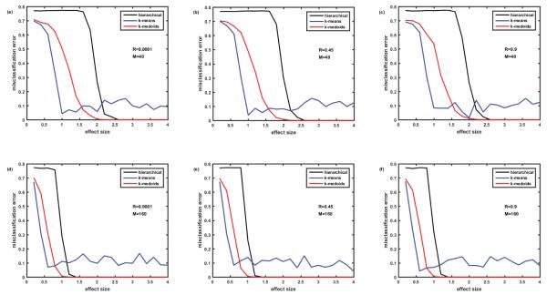
Below we demonstrate the results of the described simulations for several settings: three popular clustering methods, various numbers of biomarkers and disease subtypes, two correlation structures, and three levels of correlation between the assayed proteins. Although the settings used here are simplified versions of the true unknown associations and effects, by exploring a range of likely scenarios, the simulation results can provide useful guidance and estimates for the more complex real life situations. We used misclassification error as a main metrics for evaluating the quality of classification for the above various methods and conditions. Misclassification error was calculated by comparing the class membership predicted by the classification methods with the known class membership in the simulated data. Misclassification error was evaluated by the ‘in house’ developed function estmisclrate.m available as supplementary file. Initially (Figures 2-10), we explored and compared the properties of the clustering algorithms when the information on the true number of clusters (subtypes of disease) is known to the algorithm while the class membership is unknown, and then we explored the more complex case (Figure 11) where the number of the clusters is unknown and determined by the clustering algorithms.

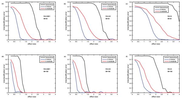
Figure 2.

Comparison of misclassification errors generated by three clustering algorithms: hierarchical, k-means, and k-medoids. Cohort of 100 simulated patients consists of 5 clusters (subtypes of disease) of equal size. Protein assay includes 1129 target proteins. Protein abundances are correlated ‘within groups’ of five. Case of non-overlapping biomarker signatures. Misclassification error=0 - means all the simulated patients are classified correctly. Misclassification error=0.8 – means only 20% of patients are classified correctly. In case of 5 clusters, this is the classification that occurs due to pure chance. Figures 2A-2C –M=40 biomarkers in the signature. Figures 2D-2F –M=160 biomarkers in the signature. Figures 2A and 2D – correlation coefficient R=0.0001, Figures 2B and 2E – R=0.45, Figures 2C and 2F – R=0.9. Here and everywhere below, each point is an average of 12 simulations.

Figure 10.

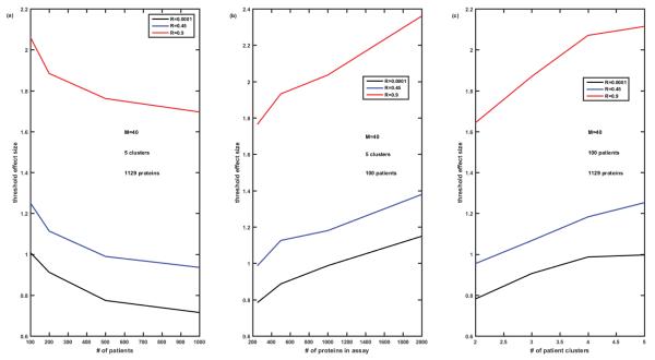
Threshold effect size enabling misclassification error below 5% for the fixed number of biomarkers in the signature M=40, versus the number P of patients (Figure 10A), versus the number N of proteins in the assay (Figure 10B), and versus the number K of clusters of patients (Figure 10C). Completely overlapping signatures, ‘among neighbors’ correlation of proteins R_ij=R^∣i-j∣. Cases of R=0.0001, 0.45, and 0.9 are compared.

Figure 11.

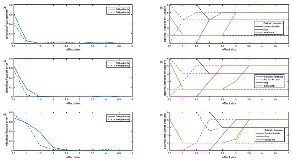
On the determination of the right number of clusters. Figures 11A, 11C and 11E misclassification error versus effect size when the correct number of clusters (five) is known and provided to the k-means algorithm (R=0.0001, 0.45 and 0.9). Number of patients P=100, 500. Number of proteins in the assay N=1129. Completely overlapping signatures, ‘among neighbors’ correlation of proteins R_ij=R^∣i-j∣. Figures 11B, 11D and 11F illustrate the situation where the correct number of clusters is not provided to the k-means algorithm but is evaluated by the evalclusters.m function based on the values of 4 criteria: Calinski-Harabasz, Davies-Bouldin, Gap and Silhoutte. Note that as everywhere in this paper, each point is an average of 12 simulations; therefore the optimal number of clusters is not necessary integer number. Note that Gap criterion performs much better than the rest of criteria, but even for Gap the required effect size for correct prediction of the number of clusters is substantially higher than the one required for correct classification when the number of clusters is known.

Results

The log(abundances) of 1129 proteins for a cohort of 100 virtual patients were simulated assuming 5 clusters of patients with equal size (20 patients in each). The effect size, i.e., the difference between the mean log(abundance) of the biomarker in the disease and control, varied from 0.2 to 4 (i.e., from 0.2 standard deviations to 4 standard deviations). Each simulation was performed at least 12 times (with different seeds generating different random distributions of protein abundances using the mvrnd.m function) and the average misclassification error was calculated.

Correlation of abundances within protein groups. Non-overlapping biomarker signatures

First we examined the case where the correlation between the protein abundances existed only within certain groups. We simulated it by assuming that all 1129 proteins can be divided into groups of 5 (actually the last group had only 4) members. Abundances of the proteins within the groups were correlated with the correlation coefficient R, while the abundances outside of the groups were not correlated.

Initially we studied the case of non-overlapping biomarkers signatures, where each cluster (disease subtype) is characterized by its own M differentially abundant proteins non- overlapping with other M differentially abundant proteins of another cluster. Figure 2 presents the comparison of misclassification errors generated by 3 clustering methods: hierarchical, k- means, and k-medoids (all with the default settings of MATLAB 2015a). Figures 2A-2C illustrate the case where the number of biomarkers in the signature M=40, while Figure 2D-2F illustrate the case of 4-fold higher number of biomarkers M=160. Figures 2A and 2D present the case of nearly zero correlation of the proteins, while Figures 2B and 2E present moderate correlation R=0.45, and Figures 2C and 2F strong correlation (R=0.9) of the protein abundances within the group of 5. In all 6 cases, hierarchical clustering generated a misclassification error rate of almost 80% until reaching a high effect size of 2.2 (M=40, Figures 2A-2C) and 1.2 (M=160, Figures 2D-2F). Note that with 5 clusters of equal size, the misclassification error of 80% (or the 20% correct classification) corresponds to classification by pure chance; therefore hierarchical clustering seems useless when the effect size is below a threshold value (2.2 where M=40 and 1.2 where M=160). However, for the larger effect sizes (above thresholds) hierarchical clustering generates nearly perfect classification. Misclassification error is lower and, therefore, classification is better with the k-medoids method for all effect sizes; classification thresholds being at effect size 2.0 for M=40 and effect size 1.0 for M=160. The slight increase of misclassification error in the setting of strong correlation of ‘within group’ protein abundances is visible when comparing k-medoids curves in Figures 2A and 2C.

The most interesting effect revealed in Figure 2 is the behavior of the misclassification error rate for the k-means method, which is substantially lower than for hierarchical and k-medoids methods for small effect sizes, but fluctuates around 10% level for large effect size, where both hierarchical and k-medoids methods provide ideal classification. This unexpected behavior of k-means method for the large effect size required further examination, which is described below.

What is wrong with k-means and how to fix it?

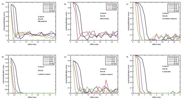
Figure 3 demonstrates our efforts to better understand the results of the k-means method as applied to our datasets. First, we increased the number of virtual patients from 100 to 500, hoping that larger sample size could help to reduce the fluctuating misclassification error at large effect sizes; it did not work (Figure 3A). Then we reduced the total number of proteins in the simulated assay from 1129 to 500, assuming that it could reduce the noise level and therefore help to classify better; it did not work either (Figure 3B). The attempts to reduce error by changing the definition of distance from the default ‘euclidian’ to ‘correlation’ (Figure 3C) and ‘city block’ (data not shown) failed as well; not surprisingly ‘city block’ distance resulted in much worse misclassification error both at small and large effect sizes. Simulating 2 patient clusters instead of 5 resulted in the disappearance of the fluctuating misclassification errors (Figure 3D), however, adding one more patient cluster (Figure 3E) resulted in the return of this type of error at large effect size.

Figure 3.

Solving the ‘puzzle of k-means behavior’. Attempts to reduce misclassification errors generated by k-means at large effect sizes (see oscillations around 10% error rates in Figure 2). Figure 3A- number of patients increased from 100 to 500; 3B- number of proteins reduced from 1129 to 500; 3C- correlation distance used instead of Euclidian distance; 3D – number of patient clusters reduced from 5 to 2; 3E- number of patient clusters=3; 3F-K- means settings are changed from default (no replicates) to 5 replicates – problem solved.

The problem of the fluctuating error of k-means was solved by looking into the details of the algorithm and comparing it with hierarchical clustering and k-medoids. Hierarchical clustering algorithm is deterministic and produces the same results every time it is run on the same data. On the contrary, k-means is a stochastic algorithm and its results depend on the seeds – the initial randomly chosen centroids of the clusters, which could be unfortunate and lead to the errors in clustering. k-medoids is similar to k-means; however in k-medoids, the centroid (called medoid) is always one of the actual data points of the cluster, which makes algorithm more robust and less dependent on initial choice of the seeds. On the other hand, at least for the data sets that we simulated, k-medoids typically resulted in a higher misclassification error than k-means (see Figures 2-6). Luckily, the k-means algorithm as implemented in MATLAB has an option of using ‘replicates’, i.e., repeat clustering multiple times using new seeds - initial cluster centroid positions and then selecting solution with the minimum value of within cluster sum of distances from points to centroid. Using this option with 5 replicates (instead of the default without replicates) dramatically reduced the fluctuating misclassification error (Figure 3F). Based on these results, k-means algorithm with 8 replicates was used in all the rest of the simulations of this paper. This was an important lesson not to rely on default settings of the algorithm, but examine and optimize its properties for the specific analytical problem. As obvious from Figures 2 and 3F, k-means algorithm with replicates proved to be the best among three classification methods for our simulated data. As shown below, the same was right for the overlapping biomarker signatures and another structure (‘among neighbors’) of the correlation matrix.

Figure 6.

Comparison of misclassification error rates generated by three clustering algorithms: hierarchical, k-means, and k-medoids. Cohort of 100 simulated patients (5 clusters of equal size). Protein assay includes 1129 target proteins. Protein abundances are correlated ‘among neighbors’ - R_ij=R^∣i-j∣. Case of completely overlapping biomarker signatures. Signatures of the clusters (disease subtypes) differ by the signs of the effect (up- or down-regulation of the proteins). See details in the text. Figures 6A-6C- M=40 biomarkers in the signature. Figures 6D-6F– M=160 biomarkers in the signature. Figures 6A and 6D– correlation coefficient R=0.0001, Figures 6B and 6E– R=0.45, Figures 6C and 6F– R=0.9.

Correlation of abundances within protein groups, overlapping biomarker signatures

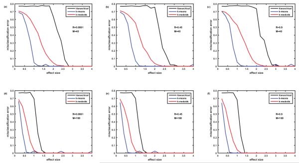
Having solved the ‘puzzle of the k-means behavior’, we moved to the simulation of the case of overlapping biomarker signatures. Here, we assumed that there were only M differentially abundant proteins in the whole protein abundance matrix and that the difference between the signatures of the patient clusters was in the level of abundance for each of the M differentially abundant proteins. In order to reduce combinatorial complexity of all possible combinations of effect sizes for M proteins, we assumed that the effect size for all the differentially abundant proteins was equal (as described in the end of the Methods section). Therefore, the logarithms of abundances of the up-regulated proteins were simulated as having effect size +Eff, while logarithms of abundances of down-regulated proteins were described with negative effect size −Eff. Even with this simplification, the number of possible distinct signature is then equal to 2^M since each of the differentially abundant proteins can be either up- or down- regulated. To simulate the expected number of disease subtypes (e.g. 5 as in previous section) we do not need this large number of signatures, so we assumed that M biomarkers are divided into 3 groups of uniformly up- or down-regulated proteins so that the max number of signatures is equal to 2³ and can be represented as sequence of pluses and minuses, e.g. +++, −−−, ++−, −+−, etc. Figure 4 represents the dependence of the misclassification error for the case of overlapping biomarker signatures described above. The structure of the figure is the same as Figure 2, i.e., it presents the comparison of 3 clustering methods. Figures 4A-4C deal with the case of M=40, while in Figures 4D-4F, M=160; Figures 4A and 4D present the case of no correlation, Figures 4B and 4Ee – moderate correlation R=0.45, and Figures 4C and 4F – strong correlation R=0.9. Note that correlation of protein abundances is simulated in the same way as for non-overlapping biomarkers (Figure 2). Comparison of Figures 2 and 4 shows that in both cases k-means is the best and hierarchical clustering is the worst in terms of misclassification error. Even the presence of very strong (R=0.9) correlations in protein abundances within the groups of proteins (here 5 proteins in the groups) causes some but not substantial increase in the misclassification error with k-means clustering. The presence of overlap in the biomarker signatures (Figure 4 versus Figure 2) causes some increase of misclassification error especially in case of low number of biomarkers M=40 (Figures 4A-4C versus Figure 2A-2C). The k-means algorithm seems to be the most robust to correlations and overlap in biomarker signatures and provide the misclassification error below 5% at effect size>1.2 for M=40 and at effect size >0.7 for M=160.

Figure 4.

Comparison of misclassification error rates generated by three clustering algorithms: hierarchical, k-means and k-medoids. Cohort of 100 simulated patients (5 clusters of equal size). Protein assay includes 1129 target proteins. Protein abundances are correlated ‘within groups’ of five. Case of completely overlapping biomarker signatures. Signatures of the clusters (disease subtypes) differ by the signs of the effect (up- or down-regulation of the proteins). See details in the text. Figures 4A-4C– M=40 biomarkers in the signature. Figures 4D-4F– M=160 biomarkers in the signature. Figures 4A and 4D– correlation coefficient R=0.0001, Figures 4B and 4E– R=0.45, Figures 4Cand 4F– R=0.9.

Among neighbors protein abundance correlation. Non-overlapping biomarker signatures

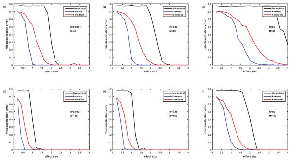
Next we examined the case, where abundances of all the proteins are to some extend correlated and are the strongest for the nearest neighbors, i.e., R_ij = R^∣i-j∣, as described in the Methods section. Figure 5 presents misclassification errors in case of this type (‘among neighbors’) of the correlation matrix and non-overlapping biomarker signatures. Comparison with the case of non-overlapping biomarker signatures and ‘within groups’ correlation of protein abundances (Figure 2), demonstrates that the ‘among neighbors’ correlation causes higher misclassification errors especially in the case of relatively low number of biomarkers M=40 (compare Figure 5B with Figure 2B, and Figure 5C with Figure 2C). Nevertheless, the k-means algorithm enables misclassification errors below 5% at effect size>1.2 for M=40 and R=0.45 and at effect size>2.2 for M=40 and R=0.9. In case of large number of biomarkers M=160, the difference of ‘among neighbors” and ‘within group’ correlations are less dramatic (compare Figure 5E with Figure 2E, and Figure 5F with Figure 2F); k-means enables misclassification error below 5% at effect size>1.2. Note that k-means algorithm enables much lower misclassification errors than k-medoids and especially hierarchical clustering algorithm. Hierarchical clustering algorithm generates especially high misclassification errors when correlation is high R=0.9, even for quite high effect sizes of 4 (M=40, Figure 5C) and 2.3 (M=160, Figure 5F).

Figure 5.

Comparison of misclassification error rates generated by three clustering algorithms: hierarchical, k-means, and k-medoids. Cohort of 100 simulated patients (5 clusters of equal size). Protein assay includes 1129 target proteins. Protein abundances are correlated ‘among neighbors’ - R_ij=R^∣i-j∣. Case of non-overlapping biomarker signatures. Figures 5A-5C– M=40 biomarkers in the signature. Figures 5D-5F– M=160 biomarkers in the signature. Figures 5A and 5D–correlation coefficient R=0.0001, Figures 5B and 5E– R=0.45, Figures 5C and 5F– R=0.9.

Among neighbors protein abundance correlation, overlapping biomarker signatures

Finally, we examined the case of overlapping biomarker signatures and ‘among neighbors’ protein abundance correlation (Figure 6). Similar to the rest of the examined cases, the k-means algorithm resulted in the lowest misclassification errors. High ‘among neighbors’ correlation resulted in the larger deterioration of performance than high ‘within group’ correlation especially in case of relatively low number of biomarkers M=40 (compare Figures 4A, 4C and 6C).

All cases k-means comparison

As shown, k-means algorithm with 8 replicates behaved better than hierarchical clustering and k-medoids for all 4 cases simulated above. Therefore it is of interest to concentrate on k-means and compare misclassification errors generated by this algorithm in the above 4 cases. Figure 7 presents this comparison. Obviously, the higher the effect size and the higher the number M of the biomarkers in the signature, the lower the misclassification error.

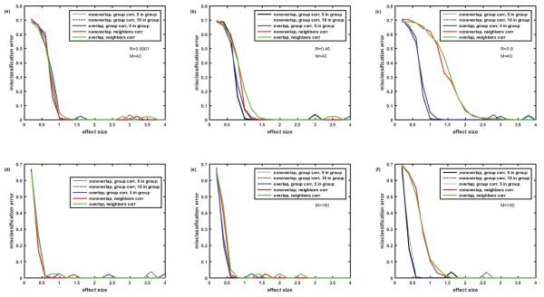
Figure 7.

Misclassification error rates generated by k-means algorithm. Cohort of 100 simulated patients (5 clusters of equal size). Protein assay includes 1129 target proteins. Comparison of 5 cases: (1)-non-overlapping signatures, correlation R within group of 5 proteins; (2)- non- overlapping signatures, correlation R within group of 10 proteins; (3)- completely overlapping signatures, correlation R within group of 5 proteins; (4)- non-overlapping signatures, ‘among neighbors’ correlation of proteins R_ij=R^∣i-j∣; (5)-completely overlapping signatures, ‘among neighbors’ correlation of proteins R_ij= R^∣i-j∣. Values of M and R are the same as in Figures 2, 4-6.

The presence of the overlap of biomarker signatures and the presence of correlation of protein abundances deteriorates the classification accuracy. However, the extend of deterioration is quite small when the correlation is low or the number of biomarkers is high M=160 (Figures 7A, 7D and 7E). Deterioration due to overlap and correlation is visible (1.5 versus 1.0 effect size threshold) when the number of biomarkers in the signature is not that high M=40 and their abundances are moderately correlated R=0.45 (Figure 7B). High correlation R=0.9 is much more detrimental in the case of ‘among neighbors’ correlation than in case of ‘within group’ correlation and results in roughly doubled effect size threshold both for M=40 (Figure 7C) and M=160 (Figure 7Ff) both in the presence or absence of biomarker signatures overlap. Also, Figure 7 illustrates that the case of protein abundance correlation within the group of 10 proteins (black dotted line) is practically indistinguishable from the case of correlation within the group of 5 proteins (black solid line).

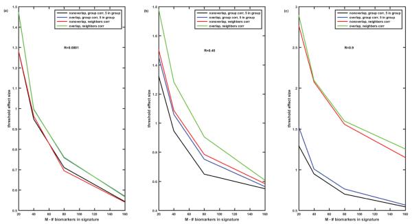
Figure 8 illustrates how the number of biomarkers in the signature influences the threshold value of the effect size which enables misclassification error below 5% for k-means algorithm. Obviously, the higher the number of the biomarkers in the signature the lower the threshold effect size required to enable misclassification error better than 5%. The value of the threshold effect size depends on the correlation of protein abundances. For low and moderate correlations of protein abundances, the discussed above 4 cases (‘overlap’ versus ‘non-overlap’ and ‘within group’ versus ‘among neighbors’) demonstrate similar dependences decreasing from 1.3-1.8 for M=20 to 0.65-0.53 for M=160 for all 4 cases (Figures 8A and 8B). However, if the correlation of protein abundances is high, cases of ‘within group’ and ‘among neighbors’ correlations differ dramatically (Figure 8C). In case of ‘within group’ correlations threshold effect size values are similar to those at Figures 8A and 8B, while in case of the ‘among neighbors’ correlations the threshold effect size values are about two-fold higher.

Figure 8.

Threshold effect size enabling misclassification error below 5% versus the number M of biomarkers in the signature. K-means algorithm. Comparison of 4 cases: (1)-non-overlapping signatures, correlation R within group of 5 proteins; (2)- completely overlapping signatures, correlation R within group of 5 proteins; (3)- non-overlapping signatures, ‘among neighbors’ correlation of proteins R_ij=R^∣i-j∣; (4)-completely overlapping signatures, ‘among neighbors’ correlation of proteins R_ij=R^∣i-j∣. Figure 8A- R=0.0001, Figure 8B– R=0.45, Figure 8C- R=0.9.

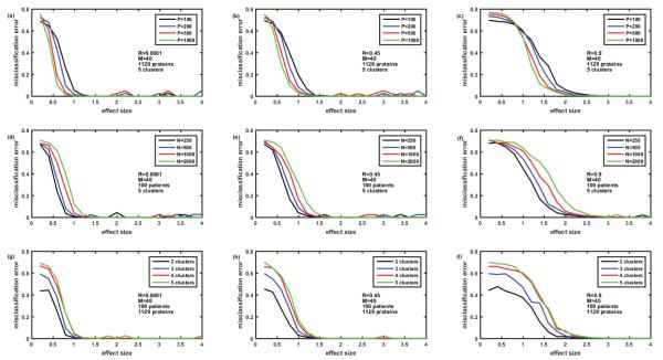
Then we analyzed the ‘worst case scenario’, i.e., overlapping biomarker signatures with ‘among neighbors’ correlation of protein abundances, in more detail. For this case, Figure 9 presents the comparison of misclassification errors generated by k-means algorithm versus the effect size for the various number of patients P=100, 200, 500, 1000 (Figures 9A-9C), various number of proteins in the panel N=250, 500, 1000, 2000 (Figures 9D-9F), and various number of patient clusters or subtypes of disease (Figures 9G-9I). The number of biomarkers in the signature is fixed M=40, and the correlation differs from R=0.0001 (Figures 9A, 9D and 9G) to R=0.45 (Figures 9B, 9E and 9H) to R=0.9 (Figures 9C, 9F and 9I). Misclassification error is lower the higher the effect size. For the given effect size misclassification error is higher the higher the correlation between protein abundances, the lower the number of patients, the higher the total number of proteins in the panel, and the higher the number of patient clusters (subtypes of disease). Importantly, these differences tend to disappear at the effect size above the threshold value, which depends on all the above parameters. Figure 10 demonstrates how the effect size threshold value enabling better than 5% misclassification error changes with the number of patients, number of proteins in the panel, number of patient clusters, and the correlation coefficient. Increasing the number of patients helps to decrease the threshold effect size but not dramatically, i.e., 10-fold increase in the number of patients lead to about 25% decrease in the value of the threshold effect size. Similarly, decreasing the number of proteins in the panel from 1000 to 200 will lead only to 20% decrease in the threshold value, while decrease in the number of patients’ clusters from 5 to 2 leads to about 25-30% decrease in the threshold effect size. The most substantial difference in the threshold value is due to the correlation of protein abundances (compare black, blue, and red curves in Figure 10). The higher the correlation the higher the threshold effect size which conforms with the dependences illustrated in Figures 8A-8C, and is not unexpected since the increased correlation coefficient is equivalent to the decrease in the number of independent biomarkers in the signature (the extreme case of R=1 being equivalent to a single biomarker M=1).

Figure 9.

Misclassification error versus effect size for various numbers P of the simulated patients in the cohort, various numbers N of proteins in the assay, and various numbers K of clusters of equal size in the cohort. K-means algorithm. M=40. R=0.0001 (Figures 9A, 9D and 9G), R=0.45 (Figures 9B, 9E and 9H) and R=0.9 (Figures 9C, 9F and 9I).

On the determination of the right number of clusters

Above, we were dealing with the situation where the clustering algorithms were provided with the information on the true number of clusters in the simulated datasets. Then we evaluated the misclassification error of these algorithms given the effect size and several other parameters of the datasets. Unfortunately, in the real life situations the true number of clusters is not always known a priori. Several criteria exist to evaluate the quality of clustering, most of which are based on the comparison of between cluster distances and within cluster distances, with the main differences between the criteria based on how these distances are defined (e.g. distances between the centroids of the clusters versus the distances between the edges of the neighboring clusters). Below we present the results of the simulation where k-means algorithm was not provided with the information on the right number of clusters (which was 5). Instead, the MATLAB function evalclusters.m was used, which calculated the values of 4 criteria (Calinski- Harabasz [18], Davies-Bouldin [19], Gap [20] and Silhoutte [21]) and made the decision on the optimal number of clusters in the given dataset based on the values of each criterion. Figure 11 presents the averaged results for 12 datasets simulating the ‘worst case scenario’ of overlapping biomarker signatures and ‘among neighbors’ correlation. A case of 100 patients is presented as a solid line, and case of 500 patients as a dashed line. Figures 11A and 11B illustrate the case of low correlation R=0.0001, Figures 11C and 11D – moderate correlation R=0.45, and Figures 11E and 11F – strong correlation R=0.9. Figures 11B, 11D and 11F present the optimal values of clusters determined based on the above 4 criteria versus the effect size, while Figures 11A, 11C and 11E present the misclassification error versus the effect size for the case where the right number of clusters (five) is known a priori and is provided to the k-means algorithm. Comparisons of Figure 11A with Figure 11B; Figure 11C with Figure 11D and Figure 11E with Figure 11F clearly illustrate that correct classification is established at much lower effect size values when the true number of clusters is known (Figures 11A, 11C and 11E) than in the cases where the optimal number of clusters is needed to be determined (Figures 11B, 11D and 11F). Comparison of the 4 criteria shows that Calinski-Harabasz criterion was consistently wrong for our datasets, predicting that the optimal number of clusters equals 2 for the range of effect sizes from 0.5 to 5. Interestingly, Davies-Bouldin criterion predicted 6 clusters for low effect size and 4 clusters for high effect size, but never predicted the correct five clusters. Gap criterion performed the best by switching from one cluster at low effect size to the correct number of 5 clusters at the moderate effect size and predicting this number consistently for the high effect size. Consistently and predictably, switching to the correct number of clusters occurred at the smaller effect size for 500 patients than for 100 patients. Performance of the Silhouette criterion looks strange: for low effect size of 0.5 it oscillates between the correct number of clusters 5 and neighboring 4 or 6 for the cases of low and moderate correlations (Figures 11B and 11D), predicts the correct number 5 for the high correlation case (Figure 11F), but then switches to the wrong number of clusters 2 for the effect sizes from 1 to 2.5-3 and only then switches back to the correct number of clusters 5 and predicts it for the high values of effect size. Without making any generalizations for other types of datasets, we conclude that Gap criterion provides the best estimate of the number of clusters in the datasets simulated in our study, i.e., omics data where the difference between clusters is reflected in the biomarker signatures, e.g. patterns of abundances of several differentially expressed proteins.

Discussion and Conclusion

In this paper, we developed an approach allowing determination of the misclassification error of popular clustering algorithms for the datasets simulating protein abundance matrices generated by targeted proteomics assays. Comparison of hierarchical, k-means, and k-medoids clustering algorithms demonstrated that k-means with several (5-8) replicates performed better than two other algorithms by enabling misclassification error below 5% at substantially lower effect size for all examined types of biomarker signatures and levels of correlations between protein abundances. Predictably, for all examined cases, the misclassification error was lower at higher effect size and with more biomarkers in the signature. Obviously, misclassification error can be decreased by increasing the number of the patients in the study and decreasing the total number of the proteins in the assay (see Figures 9 and 10). However, these effects appeared to be much less dramatic than the effect of the correlation of the protein abundances within the assay, e.g. five-fold increase of the number of patients (from 100 to 500) and two-fold decrease in the number of proteins in the assay (from 1000 to 500) lead to about 20% decrease in the threshold value of the effect size (enabling misclassification error below 5%), while two-fold increase of protein abundance correlation (from R=0.45 to R=0.9) leads to two-fold increase of the threshold effect size value. This finding is especially important since the protein abundance correlation matrix can be generated relatively easily for a given assay both from the experimental data and through pathway analysis, but is very seldom published and discussed. We hope by this publication to draw attention to the importance of the correlation matrices of omics assays.

The developed approach demonstrates that it is possible to perform power analysis for the unsupervised classification, i.e. determine the required sample size (number of patients) for the study given the expected number of subtypes of disease, number of biomarkers in the signature, effect size for each of the biomarkers, and the correlation matrix of protein abundances for the given assay. We are in the process of developing an open source online tool for this type of power analysis.

Analyses performed in this paper demonstrated that substantially higher effect size is required to determine the correct number of clusters (subtypes of disease) from the data than to correctly classify the same data when the number of clusters is known. This finding suggests that it might be beneficial to perform a two-stage classification process, where only the patients with high severity of disease (presumably higher effect sizes of biomarkers) are used for the first stage of analysis to determine the number of clusters (subtypes of disease), and then the whole cohort of patients with all severity levels is classified, given the number of clusters determined during the first stage. Obviously, this 2-stage approach has a limitation of assuming that there is the same true number of clusters for patients with severe symptoms as there are for those across the whole spectrum of symptoms. Nevertheless, it might be a useful starting point for classification in case of low effect sizes.

Several assumptions and simplifications were used in this paper, including either total non-overlap or total overlap of biomarker signatures, ‘within group’ or ‘among neighbors’ correlation of protein abundances, equal effect size of all biomarkers in the signature, and equal number of samples/patients in each cluster. These assumptions served to reduce the potential combinatorial complexity of the ‘real life’ data and are not required for the above approach to simulation of misclassification errors in clustering methods. Power analysis for each ‘real life’ case can be performed given the correlation matrix of the assay, expected ranges of effect sizes and numbers of biomarkers in the signatures for each subtype of disease. Simulation of the more complex ‘real life’ cases with unequal cluster sizes, biomarker signatures and correlation matrix structure derived from real data will be presented in our next publications. Also importantly, we plan to develop a user-friendly open source publicly available toolbox for power analysis in unsupervised and semi-supervised classification based on the above described approach. Lastly, this approach is not limited to proteomics data, or more generally to omics data, but can be used to perform power analysis of classification based on psychological tests, or self-reported measures surveys, where the correlation matrix of the questionnaire might be not less important than correlation matrix of proteomics assay.

References

- 1.Becker KG. The common variants/multiple disease hypothesis of common complex genetic disorders. Medical Hypothesis. 2004;62:309–317. doi: 10.1016/S0306-9877(03)00332-3. [DOI] [PubMed] [Google Scholar]
- 2.Relton CL, Davey Smith G. Epigenetic epidemiology of common complex disease: Prospects for prediction, prevention, and treatment. PLoS Med. 2010;7:e1000356. doi: 10.1371/journal.pmed.1000356. [DOI] [PMC free article] [PubMed] [Google Scholar]
- 3.Coyne KS, Matza LS, Kopp ZS, Thompson C, Henry D, et al. Examining lower urinary tract symptom constellations using cluster analysis. BJU Int. 2008;101:1267–1273. doi: 10.1111/j.1464-410X.2008.07598.x. [DOI] [PubMed] [Google Scholar]
- 4.Duda RO, Hart PE, Stork DG. Pattern classification. 2nd edn Wiley; New York: 2001. [Google Scholar]
- 5.Carlsson G. Topology and Data. Bulletin of the American Mathematical Society. 2009;46:255–308. [Google Scholar]
- 6.Nicolau M, Levine AJ, Carlsson G. Topology based data analysis identifies a subgroup of breast cancers with a unique mutational profile and excellent survival. Proc Natl Acad Sci U S A. 2011;108:7265–7270. doi: 10.1073/pnas.1102826108. [DOI] [PMC free article] [PubMed] [Google Scholar]
- 7.Yao Y, Sun J, Huang X, Bowman GR, Singh G, et al. Topological methods for exploring low-density states in biomolecular folding pathways. J Chem Phys. 2009;130:144115. doi: 10.1063/1.3103496. [DOI] [PMC free article] [PubMed] [Google Scholar]
- 8.Lum PY, Singh G, Lehman A, Ishkanov T, Vejdemo-Johansson M, et al. Extracting insights from the shape of complex data using topology. Sci Rep. 2013;3:1236. doi: 10.1038/srep01236. [DOI] [PMC free article] [PubMed] [Google Scholar]
- 9.Robotti E, Manfredi M, Marengo E. Biomarkers Discovery through Multivariate Statistical Methods: A Review of Recently Developed Methods and Applications in Proteomics. J Proteomics Bioinform. 2014;S3:003. [Google Scholar]
- 10.Hathout Y, Brody E, Clemens PR, Cripe L, DeLisle RK, et al. Large-scale serum protein biomarker discovery in Duchenne muscular dystrophy. Proc Natl Acad Sci U S A. 2015;112:7153–7158. doi: 10.1073/pnas.1507719112. [DOI] [PMC free article] [PubMed] [Google Scholar]
- 11.Baird GS, Nelson SK, Keeney TR, Stewart A, Williams S, et al. Age-dependent changes in the cerebrospinal fluid proteome by slow off-rate modified aptamer array. Am J Pathol. 2012;180:446–456. doi: 10.1016/j.ajpath.2011.10.024. [DOI] [PMC free article] [PubMed] [Google Scholar]
- 12.De Groote MA, Nahid P, Jarlsberg L, Johnson JL, Weiner M, et al. Elucidating novel serum biomarkers associated with pulmonary tuberculosis treatment. PLoS One. 2013;8:e61002. doi: 10.1371/journal.pone.0061002. [DOI] [PMC free article] [PubMed] [Google Scholar]
- 13.Chen R, Brentnall TA, Pan S, Cooke K, Moyes KW, et al. Quantitative Proteomics Analysis Reveals That Proteins Differentially Expressed in Chronic Pancreatitis Are Also Frequently Involved in Pancreatic Cancer. Mol Cell Proteomics. 2007;6:1331–1342. doi: 10.1074/mcp.M700072-MCP200. [DOI] [PubMed] [Google Scholar]
- 14.Andreev VP, Dwivedi RC, Paz-Filho G, Krokhin OV, Wong ML, et al. Dynamics of plasma proteome during leptin replacement therapy in genetically-based leptin deficiency. Pharmacogenomics J. 2011;11:174–190. doi: 10.1038/tpj.2010.30. [DOI] [PMC free article] [PubMed] [Google Scholar]
- 15.Andreev VP, Petyuk VA, Brewer HM, Karpievitch YV, Xie F, et al. Label-free quantitative LC-MS proteomics of Alzheimer’s disease and normally aged human brains. J Proteome Res. 2012;11:3053–3067. doi: 10.1021/pr3001546. [DOI] [PMC free article] [PubMed] [Google Scholar]
- 16.Dawson J, Walters M, Delles C, Mischak H, Mullen W. Urinary proteomics to support diagnosis of stroke. PLoS One. 2012;7:e35879. doi: 10.1371/journal.pone.0035879. [DOI] [PMC free article] [PubMed] [Google Scholar]
- 17.Good DM, Zürbig P, Argilés A, Bauer HW, Behrens G, et al. Naturally occurring human urinary peptides for use in diagnosis of chronic kidney disease. Mol Cell Proteomics. 2010;9:2424–2437. doi: 10.1074/mcp.M110.001917. [DOI] [PMC free article] [PubMed] [Google Scholar]
- 18.Calinski T, Harabasz J. A dendrite method for cluster analysis. Communications in Statistics. 1974;3:1–27. [Google Scholar]
- 19.Davies DL, Bouldin DW. A cluster separation measure. IEEE Trans Pattern Anal Mach Intell. 1979;1:224–227. [PubMed] [Google Scholar]
- 20.Tibshirani R, Walther G, Hastie T. Estimating the number of clusters in a data set via the gap statistic. Journal of the Royal Statistical Society Series B. 2001;63:411–423. [Google Scholar]
- 21.Rouseeuw PJ. Silhouettes: a graphical aid to the interpretation and validation of cluster analysis. Journal of Computational and Applied Mathematics. 1987;20:53–65. [Google Scholar]
- 22.Lu C, King RD. An investigation into the population abundance distribution of mRNAs, proteins, and metabolites in biological systems. Bioinformatics. 2009;25:2020–2027. doi: 10.1093/bioinformatics/btp360. [DOI] [PubMed] [Google Scholar]
- 23.Hair JR, Anderson RE, Tatham RL, Black WC. Multivariate Data Analysis. Prentice- Hall Inc; Upper Saddle River, NJ: 1998. [Google Scholar]
Associated Data
This section collects any data citations, data availability statements, or supplementary materials included in this article.