

Abstract
Histopathological whole-slide images (WSIs) have emerged as an objective and quantitative means for image-based disease diagnosis. However, WSIs may contain acquisition artifacts that affect downstream image feature extraction and quantitative disease diagnosis. We develop a method for detecting blur artifacts in WSIs using distributions of local blur metrics. As features, these distributions enable accurate classification of WSI regions as sharp or blurry. We evaluate our method using over 1000 portions of an endomyocardial biopsy (EMB) WSI. Results indicate that local blur metrics accurately detect blurry image regions.
INTRODUCTION
Digital histopathological whole-slide imaging (WSI) has emerged as an information-rich data acquisition method that can improve the objectivity and accuracy of disease diagnosis [1]. Although histopathology has long been a standard method for diagnosis of diseases such as cancer [2] and cardiovascular disease [3], it is often considered to be subjective [4]. Consequently, automated WSI data analysis pipelines have emerged that can improve the objectivity of image feature extraction and prediction modeling. However, due to the high resolution of WSIs, image artifacts are often present that must be detected by the image analysis pipeline. These artifacts arise due to tissue folding, slide imperfections, lighting inconsistencies, and improper calibration of imaging equipment. Automated image analysis algorithms must be able to detect these artifacts in order to ensure the fidelity of downstream image features. Previous studies have explored tissue-fold, slide imperfections, and lighting artifacts [5, 6]. In this study, we propose and evaluate a novel method for detection of blur artifacts.
Image blur is often caused by the attenuation of high spatial frequencies, which usually results when the image is compressed or filtered [7]. Blur can also occur during image acquisition. For example, in WSI, portions of the tissue slice may be unevenly aligned with the microscope focal plane. Figure 1 is an example of both sharp and blurred image portions that can occur within a single WSI of an endomyocardial biopsy (EMB). Automatic detection of image blur regions may improve the quality of diagnostic pipelines based on WSIs [8].
Fig. 1.
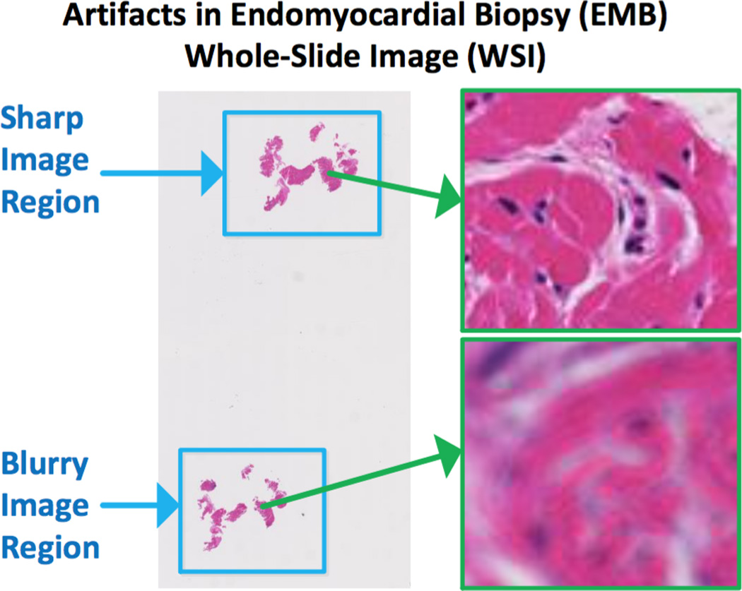
Blur artifacts in an endomyocardial biospy (EMB) whole-slide images (WSI)
Researchers generally use objective metrics to quantify the extent of blur in images. These metrics can be categorized into three types: full-reference, reduced-reference, and no-reference. In the full-reference and reduced-reference metrics, full or partial reference information about an original image is available, and an image can be compared with the reference image to determine whether it is blurred. However, such reference information is not always available. Thus, no-reference metrics are favored. No-reference metrics for blur detection characterize the extent of blurriness in a given image and assume that the distribution of the metric is different for blurry and sharp images. However, no-reference metrics have some disadvantages. These metrics tend to neglect extreme parts of an image, and thus decrease the detection accuracy. Moreover, if metrics for blurry images and sharp images have a very close or overlapping distributions, prediction accuracy will be low.
To address such issues, we propose a new blur detection workflow, which is based on “local” metrics. Instead of assigning a single no-reference metric value to one image, we calculate a metric for each pixel of the given image that captures local blur information. We then bin the distribution of all local metrics for an image to produce features that can be used to train a classifier (Figure 2).
Fig. 2.
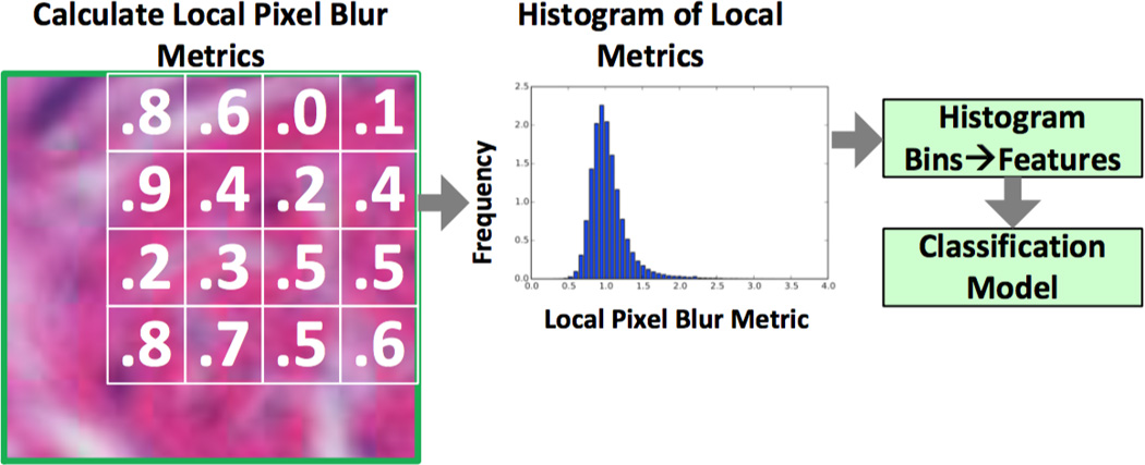
Classification of blurry and sharp images using histogram features of local blur metrics.
The rest of our paper is structured as follows: in Section II we will introduce no-reference metrics, which will also serve as baselines in our experiment. Then we explain our blur detection feature construction method in Section III. Extensive experimental results are presented in Section IV to validate the effectiveness of our method, and in Section V. we briefly discuss the future direction of our work.
METHODS
Histopathological Whole-Slide Images of Endomyocardial Biopsy
We evaluate blur detection methods using a dataset consisting of 1187 512x512-pixel tiles from a histopathological WSI image of an endomyocardial biopsy (EMB). EMBs are routinely extracted from heart transplant patients to monitor and detect transplant rejection. While WSIs can provide a large amount of information to assist pathologists with diagnosis, these image modalities are susceptible to artifacts. The particular WSI in our dataset is partially blurred. 436 of the 1187 image tiles are known to be blurred. We use these blur and non-blur labels to evaluate blur detection methods.
Global Blur Detection Metrics
Before we proceed to our method, in this section, we mainly summarized three comparison algorithms in our experiments.
Wavelet Transform Based Metric
In Tong et al. (2004), the author analyzed the linear blur model G = H * F + N, where, G,F represents blurred image and the original one, H is the blur function. The author analyzed the edge type and sharpness using Harr wavelet transform, then based on the numbers of different edge types, a global blur metric in the range [0,1] is calculated. Based on experiments, the author set a threshold, so that when the metric is smaller than the threshold, the image is classified as blur. In our experiment, we will refer it to ’Harr’ for simplicity.
No-Reference Perceptual Blur Metric
This method is proposed in Crete et al. (2007). The idea is that if a picture is already blurred, then applying a blur function will not change the quality of picture that much, compared to applying the blur function to a clear image. Based on such difference, a metric is defined in the range [0,1], when the metric is bigger than a threshold, the image is classified as blur. In our experiment, we will refer it to ’NRP’ for simplicity.
CPBD Sharpness Metric
In Bhor et al. (2014), the author illustrated a sharpness metric based on cumulative probability(CPBD). The paper first divided the original image to several blocks then examined the edge information in each block; then in each block, a probability characterizing the extent of blur is calculated according to the edge type, length in the block. Finally, the cumulative probability for scores under a threshold is obtained and this sum is used as a sharpness metric. After normalization, the blur metric in range [0,1] is defined. In our experiment, we will refer it to ’CPBD’ for simplicity.
Local Blur Detection Metrics
In our experiment, we are mainly interested in how distributions of local metric can be used to characterize the global blur information about a picture, i.e., for each pixel of the image, we will calculate a score based on itself and its neighbors, then we need to find a description for the distributions of these scores. Here we can use the histogram of these scores to approximate the probability density function of these scores.
In mathematical formulations, suppose an image has N * N pixels, we can calculate N scores for each pixels, X1,X2,…,XN2. Then we set a number of bins in constructing the histogram, say k, then the count of each bin, count1, count2,…,countk, the center of each bin, center1,…,centerk, these 2k numbers are used as features for this image. This practice is similar to the popular Histogram Oriented Dalal and Triggs (2005)
Inspired by Shi, Xu, and Jia (2014) and Bhor et al. (2014), three different scores are used in this approach, Kurtosis Measure(referred as hist_kurt in experiment), Average Power Spectrum(hist_power), Probabilistic Blur Detection Metric(hist_PBD).
Kurtosis Measure
DeCarlo (1997) detailedly describe why Kurtosis measure can be used to characterize the skewness of distributions. For a random variable X with mean μ, variance σ2, its Kurtosis measure, is defined as
Sometimes, as the Kurtosis measure for a Gaussian random variable is 3, we could also define
Power Spectrum
For an image, the average power spectrum in the frequency domain J(w), is defined as Shi, Xu, and Jia (2014)
where n is the number of different θ, (w,θ) is the polar coordinate for the pixel in the original image, J(w,θ) is the square magnitude of Discrete Fourier Transform.
The author in Shi, Xu, and Jia (2014) continues to define the power spectrum metric for a pixel as
Probabilistic Blur Detection Metric
In Narvekar and Karam (2009), the author defines a probabilistic local metric. For each pixel and its neighbors, edges in this block is calcualted and edge weights are obtained. Then for each edge ei,
where β is a defined constant, width(ei)) is the measured width for this edge, wJNB(ei) is defined in Ferzli and Karam (2009) to capture the ’Just Noticeable Blur’, using minimum amount of perceived blurriness around an edge given a contrast.
RESULTS AND DISCUSSION
Experimental Settings
After we construct these 3 sets of local metric features: Kurtosis measure (abbreviated as Kurtosis), Power Spectrum (abbreviated as Power), Cumulative Probabilistic Blur Detection Metric (abbreviated as CPBD), we can use several different classifiers to predict whether an image of blur. In this paper, we are using popular Support Vector Machine (SVM), Naïve Bayes (NB), Random Forests (RF), and k-nearest neighbors classification (KNN). The higher the classification performance, the better our features will be. We are using F1 measure, accuracy, precision, recall and area under ROC curve (AUC) as evaluation metrics, which are all calculated using 10-fold cross validation.
The 3 methods we introduced in Section II are used as baselines: Harr Wavelet Transform Based Metric (abbreviated as Harr), No Reference Perceptual Blur Metric (NRP) and CPBD Sharpness Metric (CPBD). The choices of threshold are computed based on their best performance.
Classification Result
Below are the results comparing our features against baselines using 4 different classification algorithms and 5 evaluation metrics. In each part, the left 3 columns are our features, and the right 3 columns are baselines. We can see that our features constantly outperform the baselines.
Among 3 sets of features we learned, we can see they are almost equally good, reaching a highest AUC of over 0.95.
Parameter Sensitivity Analysis
Next we present our sensitivity analysis for the parameters. Two key parameters are the number of bins we are using in constructing histograms and the size of neighbor when calculating the local metrics. Here we pick Kurtosis measure as an example. The figure shows how SVM performs when the classification performance is measured using AUC in our dataset.
When the number of neighbors is getting larger and larger, it can be seen the classification performance are getting worse. This is an intuitive result since if the number of neighbors are big enough to cover the whole image, our local metric is just a global metric, thus losing the ability to discriminate blur images from sharp ones. And when the number of bins are getting bigger with small number of neighbors, the performance are getting worse. Such pattern is rather weak when the number of bins are large.
CONCLUSION
In our current work, we have proven the effectiveness of local metric in identifying blur images, one next step will be how we can use such metrics to help restore the images.
Fig. 3.
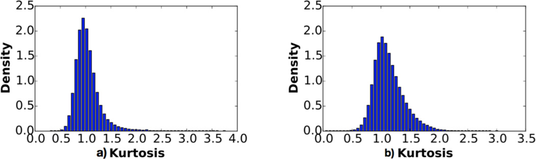
Histograms of local kurtosis in a blurry (a) and sharp (b) image.
Fig. 4.
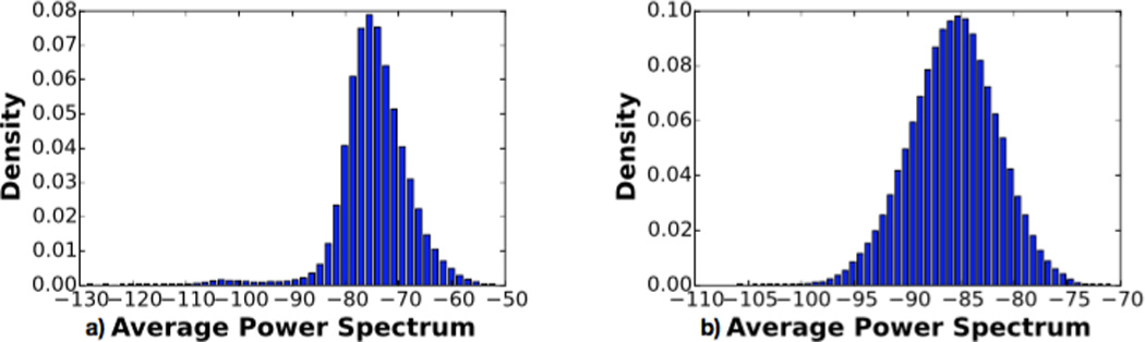
Histograms of local average power spectrum in a blurry (a) and sharp image (b).
Fig. 5.
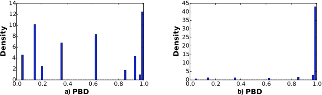
Histograms of local probablity metric in a blurry (a) and sharp image (b).
Fig. 6.
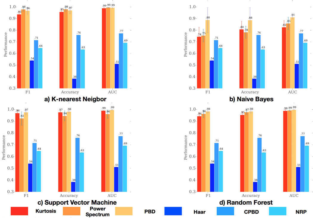
Local Pixel-Level metrics (red and orange) for detection of blurry images are more accurate compared to global metrics (blue). Results are consistent for a) KNN, b) NB, c) SVM, and d) RF; and for metrics F1-Score, Accuracy, and AUC.
Fig. 7.
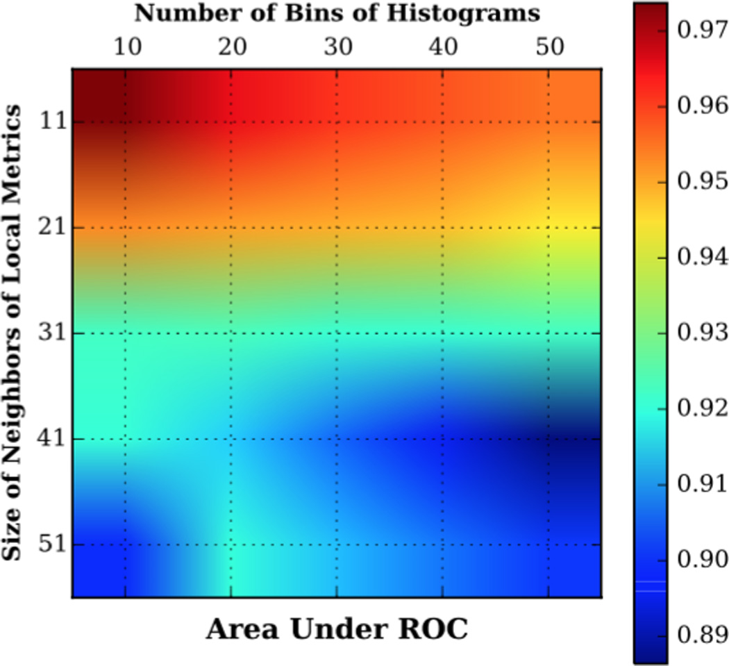
Detection of image blur using local metric is sensitive to the size of neighbors used to calculate local metrics, as well as the number of histogram bins.
Acknowledgments
This research has been supported by grants from National Institutes of Health (Center for Cancer Nanotechnology Excellence U54CA119338, and R01 CA163256), Georgia Cancer Coalition (Distinguished Cancer Scholar Award to Professor Wang).
References
- 1.Kothari S, Phan JH, Stokes TH, Wang MD. Pathology imaging informatics for quantitative analysis of whole-slide images. Journal of the American Medical Informatics Association. 2013 doi: 10.1136/amiajnl-2012-001540. amiajnl-2012-001540. [DOI] [PMC free article] [PubMed] [Google Scholar]
- 2.Gurcan MN, Boucheron LE, Can A, Madabhushi A, Rajpoot NM, Yener B. Histopathological image analysis: A review. Biomedical Engineering, IEEE Reviews in. 2009;2:147–171. doi: 10.1109/RBME.2009.2034865. [DOI] [PMC free article] [PubMed] [Google Scholar]
- 3.Stewart S, Winters GL, Fishbein MC, Tazelaar HD, Kobashigawa J, Abrams J, Andersen CB, Angelini A, Berry GJ, Burke MM. Revision of the 1990 working formulation for the standardization of nomenclature in the diagnosis of heart rejection. The Journal of heart and lung transplantation. 2005;24:1710–1720. doi: 10.1016/j.healun.2005.03.019. [DOI] [PubMed] [Google Scholar]
- 4.Ho J, Parwani AV, Jukic DM, Yagi Y, Anthony L, Gilbertson JR. Use of whole slide imaging in surgical pathology quality assurance: design and pilot validation studies. Human pathology. 2006;37:322–331. doi: 10.1016/j.humpath.2005.11.005. [DOI] [PubMed] [Google Scholar]
- 5.Kothari S, Phan J, Wang M. Eliminating tissue-fold artifacts in histopathological whole-slide images for improved image-based prediction of cancer grade. Journal of Pathology Informatics. 2013;4:22. doi: 10.4103/2153-3539.117448. [DOI] [PMC free article] [PubMed] [Google Scholar]
- 6.Hoffman R, Kothari S, Phan J, Wang MD. A High-Resolution Tile-Based Approach for Classifying Biological Regions in Whole-Slide Histopathological Images. In: Springer International Publishing, editor. The International Conference on Health Informatics. 2014. pp. 280–283. [DOI] [PMC free article] [PubMed] [Google Scholar]
- 7.Sinha U, Bui A, Taira R, Dionisio J, Morioka C, Johnson D, Kangarloo H. A review of medical imaging informatics. Annals of the New York Academy of Sciences. 2002;980:168–197. doi: 10.1111/j.1749-6632.2002.tb04896.x. [DOI] [PubMed] [Google Scholar]
- 8.Shi J, Xu L, Jia J. Discriminative blur detection features; Computer Vision and Pattern Recognition (CVPR), 2014 IEEE Conference on; 2014. pp. 2965–2972. [Google Scholar]
- 9.Tong Hanghang, Li Mingjing, Zhang Hongjiang, Zhang Changshui. Multimedia and Expo, 2004. ICME’04. 2004 IEEE International Conference on. Vol. 1. IEEE; 2004. Blur Detection for Digital Images Using Wavelet Transform; pp. 17–20. [Google Scholar]
- 10.Narvekar Niranjan D, Karam Lina J. Quality of Multimedia Experience, 2009. QoMEx 2009. International Workshop on. IEEE; 2009. A No-Reference Perceptual Image Sharpness Metric Based on a Cumulative Probability of Blur Detection; pp. 87–91. [Google Scholar]
- 11.Ferzli R, Karam LJ. A No-Reference Objective Image Sharpness Metric Based on the Notion of Just Noticeable Blur (JNB) IEEE Transactions on Image Processing. 2009;18(4):717–728. doi: 10.1109/TIP.2008.2011760. [DOI] [PubMed] [Google Scholar]
- 12.eCarlo Lawrence T. On the Meaning and Use of Kurtosis. Psychological Methods. 1997;2(3):292. [Google Scholar]
- 13.Dalal Navneet, Triggs Bill. Computer Vision and Pattern Recognition, 2005. CVPR 2005. IEEE Computer Society Conference on. Vol. 1. IEEE; 2005. Histograms of Oriented Gradients for Human Detection; pp. 886–893. [Google Scholar]
- 14.Bhor Pooja, Gargote Rupali, Vhorkate Rupali, Yawle RU, Bairagi VK. A No Reference Image Blur Detection Using Cumulative Probability Blur Detection (CPBD) Metric. [Accessed November 9];2014 [Google Scholar]