Integration of multimodal RNA-seq data for prediction of kidney cancer survival

Abstract

Kidney cancer is of prominent concern in modern medicine. Predicting patient survival is critical to patient awareness and developing a proper treatment regimens. Previous prediction models built upon molecular feature analysis are limited to just gene expression data. In this study we investigate the difference in predicting five year survival between unimodal and multimodal analysis of RNA-seq data from gene, exon, junction, and isoform modalities. Our preliminary findings report higher predictive accuracy-as measured by area under the ROC curve (AUC)-for multimodal learning when compared to unimodal learning with both support vector machine (SVM) and k-nearest neighbor (KNN) methods. The results of this study justify further research on the use of multimodal RNA-seq data to predict survival for other cancer types using a larger sample size and additional machine learning methods.

INTRODUCTION

Kidney cancer is of prominent concern in modern medicine; it is expected that 61,560 new cancer cases reported in 2015 will be localized to the kidney or renal pelvis [1]. Effective survival time prediction may provide patients with valuable perspective and inform their physicians’ course of action in developing a treatment regimen. Determining the five year survival rate for kidney cancer remains relatively unclear, as survival rate varies notably by subtype [1], [2]. Though the five year survival rate for renal cell carcinoma is 74%, for renal pelvis carcinoma this expectancy drops to 49% [1]. This inconsistency combined with the sheer variety of kidney cancer subtypes [3] and the lack of recommended screening tests for early detection [1] highlights the importance of computational models for predicting survival time of kidney cancer patients.

Several different models for predicting kidney cancer survival rates currently exist [3], [4]. Some models rely on symptoms, tumor anatomy, and time from the initial disease diagnosis [4] [5] [6] [7]; however, these models encounter many of the aforementioned prognostic limitations in subtyping, timely detection of kidney cancer, and early stage symptom recognition. Models built upon molecular feature analysis avoid these limitations and seek to identify various biomarkers that are potentially present in the body in specific amounts during the diseased state. Numerous studies have established survival models based on the presence of different biomarkers [4], [8], [9]–, but relatively little is known about the predictive power of machine learning protocols built upon the predicted outcomes of multiple different biomarker models.

Our research objective is to investigate a multi-view learning method that integrates information from multiple modalities of RNA-seq data (gene, exon, isoform, and junction). To this end, we have gathered kidney cancer RNA-seq data provided by The Cancer Genome Atlas (TCGA). It was our anticipation that integrating multimodal RNA-Seq data may provide a holistic molecular view of cancer that can potentially lead to more accurate prognostic clinical predictors of disease outcome.

BACKGROUND

Current research on designing prediction models for kidney cancer survival is largely focused on selecting pertinent data features for training machine learning algorithms. These features can be symptomatic, as with the work conducted by Kattan et al. [5] which sought to estimate five year survival using features such as tumor size, tumor node metastasis (TNM) classification, and histologic type. Similarly, the Memorial Sloan-Kettering Cancer Center (MSKCC) prediction model developed by Motzer et al. [7] and expanded upon by the Cleveland Clinic Foundation (CCF) group [6], classifies patients into risk groups ranging from favorable to poor based on the number of certain adverse factors like starting systemic therapy less than one year after diagnosis, elevated corrected serum calcium, elevated lactate dehydrogenase [LDH] level, low hemoglobin level, and low Karnofsky performance status score [4], [6], [7].

Alternatively, the increasing role of bioinformatics in the field of medicine has placed much focus on molecular feature analysis as the basis for clinical prediction modelling. The solution offered by our research involves the integration of molecular feature analysis, which may provide a means of kidney cancer model performance improvement. A study done by Jagga et al. [8] analyzed RNA-Seq gene expression data and utilized various machine learning algorithms to determine which classifier out of a group of 4 different machine learning classifiers (J48, naïve Bayes, sequential minimal optimization (SMO), and random forest) offered the best performance as measured by prediction accuracy, sensitivity, specificity, and ROC analysis [8]. 10-fold Cross Validation and Fast Correlation Based Feature (FCBF) selection methods [10] were used in analysis of gene expression profiles obtained from TCGA and the classifiers were trained using solely gene expression data. The random forest model demonstrated the best performance, resulting in an area under the receiver operating curve (AUC) of 0.876 and total accuracy of 0.797. Our study follows similar protocols with a slightly different objective-observing differences in predictive accuracy between machine learners trained on a combination of multiple genomic modalities of kidney cancer data and those trained on one modality. Employing multimodal genomic expression machine learning for prediction of kidney cancer survival rate is unique to our study and should provide a distinctive perspective on cancer prediction and the complexities that surround it.

METHODS

We have compared the survival rate predictive accuracy of integrating prediction results from four different genomic modalities of kidney cancer with the predictive accuracy attained by each modality individually. To monitor changes in predictive accuracy across different modes of machine learning, this comparison was made using prediction models built upon KNN and SVM learning methods. Predictive accuracy was evaluated using AUC, while PPV and overall accuracy (percent of correct predictions) were also observed as additional metrics for predictive accuracy.

A. RNA-Seq Kidney Cancer Data

The data analyzed in this study was acquired by TCGA using RNA-seq technology and comprised information from gene, exon, isoform, and junction modalities as depicted in Fig. 1. The initial feature size of each modality is listed in Table I. Our dataset contained genomic data from 220 kidney cancer patients labeled by survival class (survival >= 5 years = 1, survival <5 years = −1). Mapped reads from genomic data were reported as ‘Reads Per Kilobase Per Million’ (RPKM) values. As denoted in Table II, these patients were randomly divided into three groups. Training1 patients were used to cross validate and train the learners for each individual modality. These learners were in turn used to predict the survival class of each patient in Training2 and Validation. The predicted labels for the patients in Training2 were used to cross validate and train the multimodal learners which assigned predicted labels to each patient in Validation.

Fig. 1.

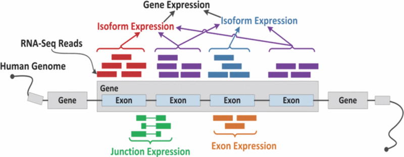
Example of gene, isoform, exon, and junction expression quantification from RNA-seq.

Table I.

Initial modality feature size

Modality	Feature Size
Gene	20531
Exon	239322
Isoform	73599
Junction	249567

Table II.

TCGA data patient stratification for kidney cancer

	Training1	Trainings2	Validation
Known Survival < 5 years	62	31	30
KnownSurvival>=5 years	49	24	24
Total Samples	111	55	54

B. Feature Selection

Given the tens of thousands of genetic features present in each modality, it was necessary to select a small number of features distinctive to each class. Minimum Redundancy Maximum Relevance (mRMR) [11] feature selection, which seeks to remove redundant features from a list of features identified as highly relevant, was utilized to extract 100 significant features. Given dataset S and class c, the mean of all mutual information values between the individual feature fi and class c is calculated to determine relevance:

$$D(\mathrm{S},c)=\frac{I}{\left|S\right|}{\displaystyle \sum _{{\mathrm{f}}_i\in S}l(F_i;c)}$$ (1)

The mean of all information values between the feature fi and the feature fj in set S is calculated to determine redundancy and thus mRMR:

$$R\mathrm{r}\mathit{SJ}=\frac{I}{|S{|}^2\mathrm{\Delta }}{\displaystyle \sum _{f_1,f_j\in S}I(f_1.f_{\mathrm{j}})}$$ (2)

$$m\mathrm{R}\mathit{MR}=ℱ[B\mathrm{G}\mathit{isc})-R(S)]$$ (3)

C. Machine Learning Methods

We selected KNN and SVM to build our preliminary prediction models in order to expand the scope of similar studies that did not explore these methods [8]. KNN classifies data into a specific class by identifying a certain number of neighbors from the training dataset that are closest to the data point in question and assigns the data point to the class associated with the most neighbors [12]. SVM defines a decision boundary that is optimized to separate two categories by a margin that is as wide as possible and assigns classes to new data points based on their position relative to the decision boundary [12].

D. Prediction Performance Metrics

Because the patient distribution in this dataset was relatively uneven (<5 years: 56%, >= 5 years: 44%), AUC was chosen to be the metric for evaluating predictive accuracy as it is independent of class prevalence. Eq. 4 shows that for Formula samples in group x and Formula. samples in group y:

$$\mathit{AUC}=\frac{1}{N+N^{-}}{\displaystyle \sum _{i=1}^{N^{+}}{\displaystyle \sum _{j=1}^{N^{-}}I(x_i>y_j)+\frac{1}{2}}}{\displaystyle \sum _{i=1}^{N^{+}}{\displaystyle \sum _{j=1}^{N^{-}}I(x_i=y_j)}}$$ (4)

where I(x) evaluates to 1 if x is true and 0 if x is false. As additional metrics for prediction, positive predictive value (PPV) and total accuracy were also reported.

$$\mathit{PPV}=\frac{\mathit{Number}\mathit{of}\mathit{True}\mathit{Positives}}{\mathit{Number}\mathit{of}\mathit{True}\mathit{Positives}+\mathit{Number}\mathit{of}\mathit{False}\mathit{Positives}}$$ (5)

$$\mathit{Total}\mathit{Accuracy}=\frac{\mathit{Number}\mathit{Correctly}\mathit{Identified}}{\mathit{Total}\mathit{Samples}}$$ (6)

E. Cross Validation to Optimize Learning Parameters

Cross validation is necessary to establish optimal learning parameters prior to training machine learners [13]. As Fig. 2 highlights, prior to training the unimodal learners, a 3-fold cross validation was conducted in which the Training1 dataset was divided into 3 subsets of equal patient distribution. One subset was designated a testing set while the other two were joined into one training set. These subsets were then used to iteratively determine the feature size (and k value for KNN) that yielded the highest predictive accuracy. This process was repeated twice more with the two other combinations of testing and training subsets, yielding two more optimal feature sizes and k values. Final optimized parameters were obtained by rounding the mean of these parameters. Similarly, prior to training the multimodal learner, a 3-fold cross validation was conducted to establish an optimized k value and list of modalities. A linear kernel was assumed for SVM learning.

Fig. 2.

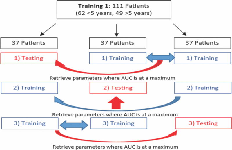
Schematic for 3-fold cross validation

F. Building Machine Learners

Using the optimized parameters identified during cross validation, KNN and SVM unimodal learners trained on the data from Training1 assigned predicted labels for the patients in Training2 and Validation for all four modalities, and AUC, PPV, and total accuracy for each were recorded. The predicted labels from each modality were then assembled into a 4-by-n matrix (n = number of samples in Training2, see Fig. 3) to cross validate and train KNN and SVM multimodal learners.

Fig. 3.

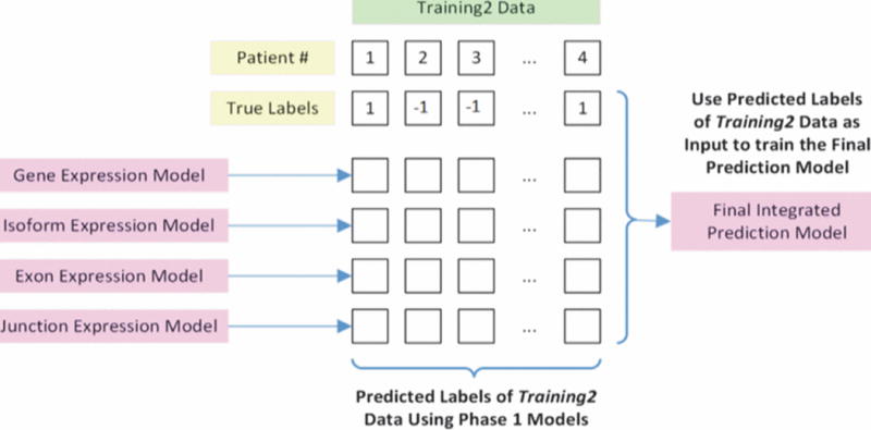
Generation of the final integrated prediction model using outputs from the unimodal prediction models

The multimodal learners assigned predicted labels to the patients in the Validation set using its matrix of unimodal predicted labels. AUC, PPV, and total accuracy were recorded for multimodal prediction and compared to the results obtained from unimodal prediction.

RESULTS

A. Cross Validation

The results of unimodal KNN and SVM cross validation are reported in Tables III and IV. Fig. 4 shows an example cross validation plot where each color represents a different iteration in the cross validation process and each point indicates an optimal k value for a particular feature size.

Table III.

Optimized unimodal KNN learning parameters

Modality	Optimized k value	Optimized feature size
Gene	29	53
Exon	31	64
Isoform	15	55
Junction	21	78

Table IV.

Optimized unimodal SVM learning parameters

Modality	Optimized feature size
Gene	6
Exorr	37
Isoform	88
unction	86

Fig. 4.

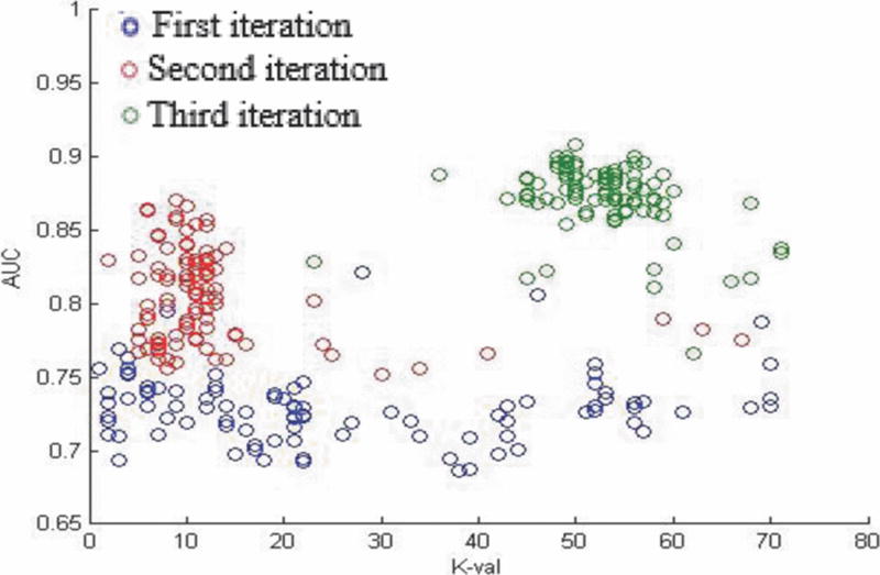
K value cross validation plot for gene modality KNN learner.

A cross validation step was also performed prior to multimodal learning to determine the optimum number of modalities and, for KNN, k value to use when training multimodal learners. Utilizing all four modalities proved to be most optimal for SVM and KNN. An optimized k value of 15 was reported for the multimodal KNN learner.

Optimized learning parameters were taken as the mean of the parameters that yielded the highest AUC value from each cross validation iteration. For KNN cross validation, the combination of k value and feature size that yielded the highest AUC were taken as optimal parameters. To evaluate cross validation performance, the mean of the maximal AUC reported in each iteration was recorded. KNN cross validation reported maximal AUC values of 0.8669, 0.8437, 0.9015, and 0.9960 for gene, exon, isoform, and junction modalities respectively and 0.9222 for multimodal cross validation. SVM cross validation reported maximal AUC values of 0.7778,0.7206,0.9015, and 0.9319 for gene, exon, isoform, and junction modalities respectively and 0.9222 for multimodal cross validation.

B. Predictive Accuracy

The optimized parameters obtained from cross validation were used as inputs for machine learning. Using Training1 as the unimodal training data set, predicted labels were obtained for patients in the Validation and Training2 datasets. For KNN, predicted labels were weighted from −1 to 1 by summing the labels (either 1 or −1) of the k nearest neighbors to each patient and dividing by k. SVM learners reported predicted labels as 1 or −1. Predictive accuracy was determined by comparing the predicted patient class labels assigned by each machine learner with each patient’s known class label. The AUC PPV, and total accuracy of each KNN and SVM machine learner are reported in Tables V and VI and Fig. 5 and 6.

Table V.

Predictive accuracy of KNN learners

Modality	AUC	PPV	Total accuracy
Multimodal	0.6444	0.7037	0.6481
Gate	0.6389	0.6897	0.6481
Exon	0.5799	0.6667	0.6111
Isoform	0.5924	0.6522	0.5741
Junction	0.6292	0.6250	0.5926

Table VI.

Predictive accuracy of SVM learners

Modality	AUC	PPV	Total accuracy
Multimodal	0.6042	0.6452	0.6111
Gene	0.6000	0.6667	0.5926
Exon	0.5375	0.5926	0.5370
Isoform	0.4792	0.5357	0.4815
Junction	0.5942	0.5588	0.5185

Fig. 5.

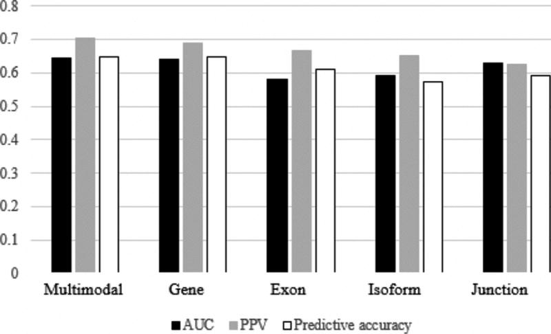
Predictive accuracy of KNN learners

Fig. 6.

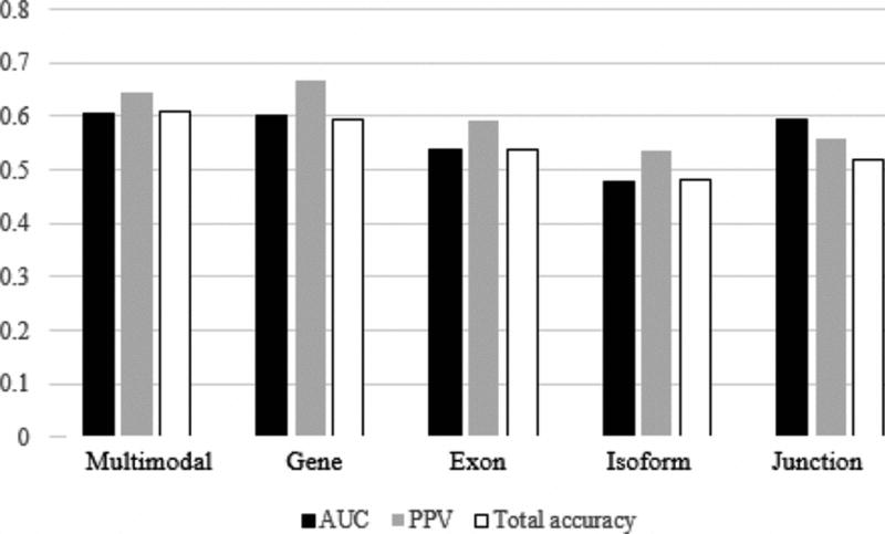
Predictive accuracy of KNN learners

The results of our analysis are promising, as AUC was greater in comparison to all unimodal learning methods for both KNN (AUC = 0.6444) and SVM (AUC = 0.6042) learning methods. What is more, KNN multimodal learning lead to a total accuracy (0.6481) and PPV (0.7037) greater than or equal to all unimodal learners, while SVM multimodal learning lead to a total accuracy (0.6111) greater than all unimodal learners and a PPV (0.6452) second only to the gene modality learner (PPV = 0.6667). Though small, a distinct increase in predictive accuracy associated with multimodal learning has been noted across multiple machine learning platforms and suggests that multimodal machine learning may augment the power of clinical prediction modelling.

DISCUSSION

The results of this study show promise for multiple reasons. Not only have we demonstrated the potential that multimodal machine learning holds for improving predictive accuracy, but we have also observed such a trend using two different machine learning methods. This observation illustrates that multimodal learning may lead to improvements in predictive accuracy across a multitude of different machine learning techniques. Our findings suggest that the predictive accuracy of existing high performance prediction models may be enhanced by our multimodal process. Such enhancements provide physicians and patients with a more informed perspective on the course of action for effective disease management. Furthermore, our findings may extend to the prediction of other clinical endpoints that can be characterized by genomic data.

The limitations of this study include: First, the sample size of our training and validation data is rather small, and thus mislabeling a small number of patients can have a big impact on predictive accuracy. However, it is our anticipation that increasing the sample size will affect the performance of multimodal and unimodal learners similarly. Second, our study was limited to two machine learning methods, and thus the notion that multimodal learning will work as effectively with other machine learning methods has not been confirmed. Third, it remains unclear if our process will yield similar results for predicting the survival time of other cancer types. In light of these limitations, further work is underway that extends our process to other cancer types and incorporates additional machine learning methods.

CONCLUSION

We have provided preliminary evidence suggesting that multimodal learning, which uses the predicted labels from machine learners trained on data from four different genomic modalities as the basis for learning, more accurately predicts the expected five year survival of kidney cancer patients compared to learning with just one modality. That the difference in predictive accuracy between the multimodal and highest performing unimodal processes is observed using two different machine learning methods warrants further research to validate our preliminary results. To that end, we are currently expanding the scope of our investigation on the predictive implications of multimodal learning to incorporate ovarian cancer data, additional cross validation steps to optimize parameters which were assumed to have negligible effects on predictive accuracy, and other machine learning methods featured in comparable research studies [8] such as random forest and naïve Bayes predictors.

References

- 1.Cancer Facts & Figures 2015. 2015 [Google Scholar]
- 2.Luke C, Sargent N, Pittman K, Price T, Roder D. Epidemiology of Cancers of the Kidney in an Australian Population. Asian Pacific Journal of Cancer Prevention. 2011;12:2893–2899. [PubMed] [Google Scholar]
- 3.Su Kim D, Choi YD, Moon M, Kang S, Lim J-B, Kim KM. Composite three-marker assay for early detection of kidney cancer. Cancer epidemiology, biomarkers & prevention: a publication of the American Association for Cancer Research, cosponsored by the American Society of Preventive Oncology. 2013;22:390–8. doi: 10.1158/1055-9965.EPI-12-1156. [DOI] [PubMed] [Google Scholar]
- 4.Finley DS, Pantuck AJ, Belldegrun AS. Tumor Biology and Prognostic Factors in Renal Cell Carcinoma. Oncologist. 2011;16:4–13. doi: 10.1634/theoncologist.2011-S2-04. [DOI] [PMC free article] [PubMed] [Google Scholar]
- 5.Kattan MW, Reuter V, Motzer RJ, Katz J, Russo P. A postoperative prognostic nomogram for renal cell carcinoma. Journal of Urology. 2001;166:63–67. [PubMed] [Google Scholar]
- 6.Mekhail TM, Abou-Jawde RM, BouMerhi G, Malhi S, Wood L, Elson P. Validation and extension of the Memorial Sloan-Kettering prognostic factors model for survival in patients with previously untreated metastatic renal cell carcinoma. Journal of Clinical Oncologv. 2005;23:832–841. doi: 10.1200/JCO.2005.05.179. [DOI] [PubMed] [Google Scholar]
- 7.Motzer RJ, Bukowski RM, Figlin RA, Hutson TE, Michaelson MD, Kim ST. Prognostic nomogram for sunitinib in patients with metastatic renal cell carcinoma. Cancer. 2008;113:1552–1558. doi: 10.1002/cncr.23776. [DOI] [PubMed] [Google Scholar]
- 8.Jagga Z, Gupta D. Classification models for clear cell renal carcinoma stage progression, based on tumor RNAseq expression trained supervised machine learning algorithms. BMC proceedings. 8:S2. doi: 10.1186/1753-6561-8-S6-S2. [DOI] [PMC free article] [PubMed] [Google Scholar]
- 9.Parker AS, Leibovich BC, Lohse CM, Sheinin Y, Kuntz SM, Eckel-Passow JE. Development and Evaluation of BioScore. Cancer. 2009;115:2092–2103. doi: 10.1002/cncr.24263. [DOI] [PMC free article] [PubMed] [Google Scholar]
- 10.Yu L, Liu H. Feature selection for high-dimensional data: A fast correlation-based filter solution. ICML. :856–863. [Google Scholar]
- 11.Ding C, Peng H. Minimum redundancy feature selection from microarray gene expression data. Journal of Bioinformatics and Computational Biology. 2005;3:185–205. doi: 10.1142/s0219720005001004. [DOI] [PubMed] [Google Scholar]
- 12.Kim J, Kim BS, Savarese S. Comparing image classification methods: K-nearest-neighbor and support-vector-machines. Proceedings of the 6th WSEAS international conference on Computer Engineering and Applications, and Proceedings of the 2012 American conference on Applied Mathematics [Google Scholar]
- 13.Virkar H, Stark K, Borgman J. Machine learning method for training machine, involves selecting trained learning machines that optimize performance function dependent on variables between classes, and outputting selected and trained learning machines into computer memory [Google Scholar]