

Abstract
RNA-sequencing (RNA-seq) technology has emerged as the preferred method for quantification of gene and isoform expression. Numerous RNA-seq quantification tools have been proposed and developed, bringing us closer to developing expression-based diagnostic tests based on this technology. However, because of the rapidly evolving technologies and algorithms, it is essential to establish a systematic method for evaluating the quality of RNA-seq quantification. We investigate how different RNA-seq experimental designs (i.e., variations in sequencing depth and read length) affect various quantification algorithms (i.e., HTSeq, Cufflinks, and MISO). Using simulated data, we evaluate the quantification tools based on four metrics, namely: (1) total number of usable fragments for quantification, (2) detection of genes and isoforms, (3) correlation, and (4) accuracy of expression quantification with respect to the ground truth. Results show that Cufflinks is able to use the largest number of fragments for quantification, leading to better detection of genes and isoforms. However, HTSeq produces more accurate expression estimates. Moreover, each quantification algorithm is affected differently by varying sequencing depth and read length, suggesting that the selection of quantification algorithms should be application-dependent.
1. INTRODUCTION
RNA-sequencing (RNA-seq), one of the most promising technologies in the current -omics era, uses deep sequencing to characterize and quantify complex transcriptomes [1]. Since its inception, RNA-seq technology has quickly progressed because of its potential benefits to human health care via gene and isoform expression profiling, allele specific expression, single nucleotide variation discovery, fusion gene detection, RNA-editing, novel transcript identification, and differential expression analysis [2–6]. Moreover, RNA-seq is gradually overshadowing microarrays in some applications and continues to overcome microarray-related challenges. Features that make RNA-seq an attractive technology compared to microarrays include (1) ability to detect alternative splice sites and novel isoforms, (2) de novo analysis of samples without a reference, (3) minimal cross-hybridization errors, and (4) single nucleotide resolution [2].
An important application of RNA-seq is gene and isoform expression profiling. Accurate gene or isoform expression profiling is critical for developing reliable clinical or biological applications such as identification of differentially expressed genes or gene expression-based prediction. However, RNA-seq expression profiling is challenging, and numerous expression quantification tools have attempted to overcome these challenges to produce accurate expression estimates.
One of the challenges is a result of repetitive sequences, especially in the human genome. RNA-seq technology is currently limited in terms of read length relative to RNA molecule length. Thus, if not handled correctly, short reads from repetitive regions may be erroneously aligned, leading to decreased performance of simple quantification tools. However, recent quantification tools are able to handle reads that align to multiple locations. These tools can use multiple alignment information to quantify expression values [7].
Another challenge for quantification is the ability to distinguish between reads from common exonic regions of a gene. As a gene is composed of multiple isoforms and each isoform consists of multiple exons of a gene, there are a number of exons that coexist in multiple isoforms. Hence, when quantifying two isoforms of a gene with common exonic regions, it is difficult to infer the origin of reads with respect to the isoforms.
Because of the rapidly evolving sequencing technology, researchers are continuously developing new library preparation protocols and downstream software tools to enhance quality of sequencing data and accuracy and efficiency of data analysis, respectively. With advances in technology and decreases in cost, the future trend will be to design application-specific experimental designs and computational data analysis pipelines. Thus, there is a need to evaluate the effect of different RNA-seq experimental designs on downstream expression quantification in order to answer the following questions. For a specific experimental design, which quantification tool will produce more accurate results? For a specific quantification tool, what is the ideal read length and sequencing depth? To address these questions, we simulate different read conditions and assess the behavior of three quantification tools using four metrics: (1) number of usable fragments, (2) ability to detect genes and isoforms, (3) correlation of expression with true expression, and (4) accuracy of expression.
2. METHODS
We use simulated data to remove unexplained variability and because the ground-truth expression values are necessary to evaluate quantification performance. The experimental procedure includes four stages (Figure 1): (1) Read Simulation, (2) Sequence Alignment, (3) Quantification, and (4) Evaluation.
Figure 1.

Experimental procedure and data analysis workflow.
2.1 Simulation of RNA-seq Data
We apply the RNASeqReadSimulator (update 2012.04.30) to generate synthetic RNA-seq data because it allows users full flexibility in controlling the read generation process. It also provides information about the transcript of origin for each read. RNASeqReadSimulator uses a number of Python scripts to generate reads based on parameters such as the distribution of the expression profiles, number of reads to be generated, read length, positional bias profile, average insert-length and standard deviation for paired-end reads, strand-specific protocol flag, and positional error profile.
We use a BED-formatted Ensembl annotation with a fixed set of randomly assigned weights (corresponding to expression magnitude) to generate paired-end reads with uniform per base positional error and bias profiles [8]. Reads are simulated for the following library preparation conditions: (1) Constant read length at 2×100bp paired-end with various sequencing depths (3 million fragments, 15 million fragments, 50 million fragments, or 100 million fragments) and (2) Constant sequencing depth at 50 million fragments and with read length of 2×50bp, 2×75bp, or 2×100bp paired-end. All conditions are generated using an average fragment length of 225bp with a 25bp standard deviation.
We adopt Ensembl GRCh37 version 67 as the genome annotation source for this study. The raw annotation file is processed to include annotations on chromosomes 1–22, chromosome X, chromosome Y, and mitochondrion only. The corresponding reference FASTA file is also downloaded from Ensembl and used for data simulation.
2.2 Sequence Alignment
After simulating RNA-seq data, the second step in our workflow is sequence alignment. We apply TopHat [4], a spliced alignment tool, to align the simulated reads to the reference genome. We use TopHat (version 2.0.6) with two different parameter settings: (1) the annotation file is ignored and the reads are directly mapped to the genome and (2) the annotation file is provided and the reads are forced to align to the transcriptome only. TopHat performs gapped alignment using Bowtie2, followed by spliced alignment. The mapped reads are reported in terms of genomic coordinates and sorted by mapping coordinates in a BAM file format.
2.3 Expression Quantification
In our workflow, we use three alignment scenarios leading to expression quantification: (1) basic counts of the origin of reads (i.e., true expression counts), (2) reads mapped to the genome using TopHat, and (3) reads mapped to the transcriptome using TopHat. Henceforth, the true expression counts serve as the reference for evaluating quantification tools. After preprocessing steps, the TopHat alignment files are quantified with HTSeq, Cufflinks, and MISO [7,9,10]. For the purpose of comparing directly against the true expression counts and keeping the quantification independent from normalization, the fragment counts reported by each quantification tool are used for evaluation.
2.3.1 Quantification Using TopHat-Mapped Reads
HTSeq (version 0.5.4p1) employs a naive count-based approach for quantification. It is limited to quantifying expression only at the gene level. The BAM file generated by TopHat is converted to SAM format and sorted by read name using SAMtools. We apply HTSeq in the intersection-nonempty and non-strand-specific mode. The reads quantified by HTSeq must originate from one location only, i.e., the origin of a read must be unique.
Cufflinks (version 2.0.2) uses a maximum likelihood-based approach to quantify expression at the gene and isoform levels. Using the Cuffdiff program, part of the Cufflinks package, it is possible to retrieve the raw read counts used by Cufflinks for quantification. Preprocessing of the TopHat alignment data is not required for using Cufflinks as it is already sorted by read- coordinates and is in BAM format. The read counts are reported for isoforms and genes separately.
MISO (Mixture of Isoforms, version 0.4.6) is a quantification tool based on Bayesian inference. It is said to perform well in the case of low-expressing genes as it provides a confidence estimate with the quantification [11]. MISO requires an index file of the coordinate sorted BAM file for its quantification. Before the quantification step, MISO indexes the annotation file. As part of the default settings, MISO requires at least 20 reads to originate from a gene for quantification. We keep this default setting to observe any resulting increases in quantification accuracy. MISO reports the number of reads it assigns to each isoform to produce isoform expression counts. Summing the count data of the isoforms of a gene will result in the gene count.
2.3.2 True Expression Counts
The read name assigned by RNASeqReadSimulator contains the transcript-id from which it originated. Using this feature of the simulated data, we calculate the true expression count for every transcript. We then identify genes related to isoforms and sum isoform read counts belonging to a particular gene to obtain the true expression count for the gene.
2.4 Data Analysis
The last step in the RNA-seq workflow is the evaluation of quantification tools. In this section, we evaluate the performance of each quantification tool for each simulated read condition. We use four metrics to evaluate quantification performance: (1) number of usable fragments for quantification, (2) detection of genes and isoforms, (3) correlation, and (4) accuracy of expression with respect to the true expression count.
2.4.1 Usable Fragments for Quantification
To compare the total number of reads, or fragments, that are usable by a quantification tool, we total the number of reads assigned to each transcript. Reads are counted for each tool under every scenario of varying sequencing depth, read length, and mapping strategy. Generally, more usable fragments correlate with higher gene and isoform detection.
2.4.2 Detection of Genes and Isoforms
An important aspect of expression quantification is its ability to detect low expressing genes or isoforms. More importantly, it is crucial for the quantification tool to be specific in detecting only genes or isoforms present in the sample under study.
We use three metrics to evaluate the detection of genes or isoforms. The first metric is the raw detection ability, which is measured by counting the number of expression values greater than zero, i.e., given by where Ii represents the presence or absence of the ith gene or isoform (1 denotes presence and 0 denotes absence), n is the total number of genes or isoforms in the annotation.
The second metric is the false positive detection. This occurs when a particular transcript is predicted to be present by a quantification tool but should not be present in the sequenced sample. We consider the quantification of a gene/isoform to be a false positive when the tool assigns an expression value greater than zero when the true expression count for the corresponding gene/isoform is zero.
The third metric is false negative detection. This occurs when the quantification tool reports a zero expression value for a transcript that should be present in the sequencing sample. We consider the quantification of a gene/isoform to be a false negative when the tool assigns an expression value of zero when the true expression count for that corresponding gene/isoform is greater than zero.
2.4.3 Correlation of Expression
Bivariate analysis is a measure commonly used to study the relation between two variables. We use this concept to study the relation between the true expression count and the expression counts reported by each quantification tool. We plot the expression count reported by each quantification tool against the true expression count to analyze this relationship.
To assess the quantification at low, medium, and high levels of expression, we transform the fragment count to the log scale using log2 (xi+1), where xi is the expression count of the ith gene or isoform. We calculate Pearson’s correlation coefficient (r) for each case.
2.4.4 Accuracy of Expression
Correlation enables us to compare the similarity of two sets of quantities. But to use these quantification tools for application- oriented studies, we need to know to what extent a user can trust these estimated expression values. Ideally the true expression count and the expression count estimated by a quantification tool should be similar and within an application-specific error tolerance. For each quantification tool and each simulated read condition, we count the number of genes or isoforms correctly quantified within 10% of the true expression count.
2.5 Quantification of Real RNA-Seq Data
For evaluating the performance of quantification tools using real RNA-seq, data we download the dataset SRP008482 from sequencing read archive (SRA). This dataset was used to study the human pulmonary microvascular endothelial cells when they are subject to thrombin for 6 hours [12]. The results from the study have validated the fold-changes of three genes using a TaqMan RT-qPCR assay. Here we study the effect of each quantification tool on variations in the fold-change of these genes compared to the current standard technique used for expression quantification (RT-qPCR).
3. RESULTS AND DISCUSSION
3.1 Mapping Statistics
We evaluate the mapping accuracy of the simulated reads.
Regardless of alignment to the genome or to the transcriptome, approximately 90% of the 100bp reads map accurately to the reference. A read is mapped accurately if its start coordinate, which is known from the simulation, matches with the mapping location or the mapping location plus the read length. The 75bp reads and the 50bp reads are less accurately mapped with accuracies of 87% and 81% when mapped to the genome and accuracies of 88% and 85% when mapped to the transcriptome. Shorter reads also have a higher percentage of reads that map to multiple locations (multihit). Transcriptomic mapping have a smaller percentage of multihits compared to genomic mapping.
When counting the percentage of reads that do not map to the correct location, the “error” introduced by single hit mapping is approximately 3% for all cases in the study, but the “error” introduced by multihit mapping ranges from 7% for 100bp reads to 15% for 50bp reads.
3.2 Usable Fragments for Quantification
For all quantifiers, the quantification of TopHat alignment with transcriptomic mappings generally utilizes more reads compared to the quantification of TopHat alignment with genomic mappings (Figure 2). In the case of genomic alignment, we suspect that a small portion of the reads are mapped incorrectly to the non- transcriptomic region (i.e., intronic or intergenic region), resulting in reduced availability of reads for quantification. HTSeq, Cufflinks, and MISO consistently use most of the reads for quantification regardless of the variations of read length or sequencing depth. Cufflinks always utilizes the largest number of reads among all tools compared.
Figure 2.

Number of usable fragments for quantification.
We also observe that, regardless of read length, the quantification tools use a similar number of reads, i.e. there is no major difference in the number of reads used between tools. In terms of the percentage of true fragment count, HTSeq continues to discard more reads as the sequencing depth increases, while Cufflinks scales up even with increase in sequencing depth.
3.3 Detection of Genes and Isoforms
When a quantification tool reports a fragment count of greater than zero we consider the gene or isoform to be detected. From Figure 3 we find that more genes are detected in TopHat transcriptomic alignment compared to the TopHat genomic alignment (the difference is minimal in HTSeq). MISO consistently reports less than half the number of True Gene Count since it only detects genes with at least 20 mapped reads. We observe in Figure 3 that, regardless of the read length, at a sequencing depth of 50 million paired-end reads the number of genes quantified or detected is comparable. With extensive sampling we have a better chance of getting even low expressed or less abundant transcripts. Hence, with increase in sequencing depth, more non-zero expression values are observed. The Venn diagrams (Figure 4) summarizes the commonly detected genes and compares the results between the genomic mapping conditions versus the transcriptomic mapping. We see that in the case of genomic mapping MISO has the largest number of unique detections and Cufflinks has the largest number of unique detections in the case of transcriptomic mapping.
Figure 3.

Number of genes detected.
Figure 4.
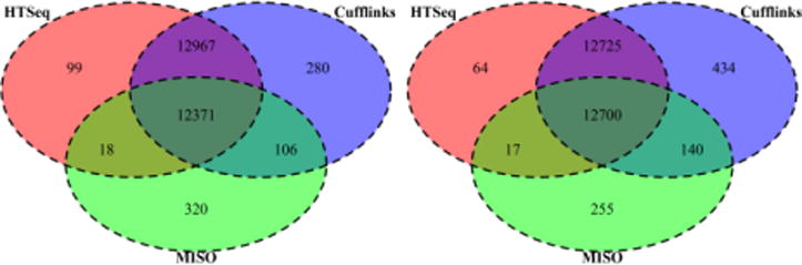
Number of commonly detected genes among different quantification tools. Venn diagrams represent the 2×100bp 100 million reads condition when mapped against the genome (left) and when mapped against the transcriptome (right). The proportions were similar in all cases of simulated reads.
We would expect the same trend in isoform detection as we observed in gene detection. However, we observe in Figure 5 that both Cufflinks and MISO detect more isoforms than the actual number present in the sample. This leads us to check for the number of false positive genes and isoforms detected by the quantification tools. HTSeq cannot detect or quantify isoforms and hence is not represented in Figure 5.
Figure 5.

Number of isoforms detected.
Considering false positive gene detections we observe from Figure 6 that variations in read length result in large changes in the number of false positive gene detections. We can clearly see that, with a decrease in read length, the number of false positives increases. This could be a result of higher mapping uncertainty due to the decreased read length as suggested by our mapping evaluation (shorter read length had higher percentage of multihit mapping). Similarly, we can explain the higher number of false positives in the case of quantification from genomic mapping compared to that of transcriptomic mapping, with the exception of the 100bp paired-end read set with a depth of 100 million fragments. Among the tools compared, Cufflinks produces the largest number of false positive genes. Figure 7 illustrates the common false positive genes detected by the three quantification algorithms. The maximum unique contribution of false positive gene detection is given by Cufflinks and MISO, leading us to believe that the majority the unique entries in Figure 4 were not accurate gene detections.
Figure 6.

Number of false positive genes.
Figure 7.

Number of common false positive genes among different quantification tools. Venn diagrams represent the 2×100bp 100 million reads condition when mapped against the genome (left) and when mapped against the transcriptome (right). The proportions were similar in all cases of simulated reads.
We then move on to counting the number of false positive isoforms detected by each quantification tool. As expected from Figure 5, we see in Figure 6 that MISO produces the largest number of false positive isoform calls.
When calculating the number of false negative genes (i.e., genes that are actually present in the read set but are not detected or quantified by the quantification tools), we observe that HTSeq and Cufflinks have very low false negative gene detection compared to that of MISO as seen in Figure 9. For the case of false negative isoforms we see in Figure 11 that it follows the same trend as that of false positive gene detection. However, in this case false negative isoforms tend to occur more frequently when mapping to the genome instead of the transcriptome.
Figure 9.

Number of false negative genes.
Figure 11.

Number of false negative isoforms.
3.4 Correlation of Expression
We then perform bivariate analysis on each read set and observe a trend for every quantification tool. We use Pearson’s coefficient to calculate the relation between the true expression count of every gene against the count data produced by the quantification tools. Table 1 summarizes the trend of the correlation for each case in the study. For HTSeq and MISO, Pearson’s correlation coefficient does not change with changes in sequencing depth while keeping the read length constant. We also see that the correlation coefficient increases with increase in read length from 50bp to 100bp paired-end reads. In contrast, we observe that, when quantifying with MISO, increases in sequencing depth increases correlation. When quantifying with HTSeq and Cufflinks, there is an increase in correlation coefficient when the read length increases.
Table 1.
Correlation of true expression and quantified expression under different conditions.
| Quantification and Mapping Strategy/Simulated Read Condition | Constant Read Length | Constant Sequencing Depth | |||||
|---|---|---|---|---|---|---|---|
| 100×2bp 3M | 100×2bp 15M | 100×2bp 50M | 100×2bp 100M | 50×2bp 50M | 75×2bp 50M | 100×2bp 50M | |
| HTSeq Genomic Mapping | 0.978 | 0.979 | 0.978 | 0.978 | 0.974 | 0.977 | 0.978 |
| HTSeq Transcriptomic Mapping | 0.985 | 0.986 | 0.986 | 0.986 | 0.982 | 0.985 | 0.986 |
| Cufflinks Genomic Mapping | 0.984 | 0.984 | 0.984 | 0.984 | 0.979 | 0.982 | 0.984 |
| Cufflinks Transcriptomic Mapping | 0.986 | 0.986 | 0.986 | 0.986 | 0.981 | 0.984 | 0.986 |
| MISO Genomic Mapping | 0.795 | 0.839 | 0.854 | 0.857 | 0.85 | 0.852 | 0.854 |
| MISO Transcriptomic Mapping | 0.806 | 0.846 | 0.859 | 0.86 | 0.854 | 0.857 | 0.859 |
Figure 12 and Figure 13 are representative scatter plots of the important observations. In Figure 13, we observe that, for HTSeq and Cufflinks, when read length is constant and sequencing depth increases, the scatter plot becomes more dispersed near the low expressing region. Support for this observation is provided by RMSE, i.e., RMSE increases with sequencing depth. With respect to genomic mapping, Cufflinks has the highest correlation coefficient. We infer from the scatter plot that there is one highly expressed gene that is not detected in any simulated read condition. On closer examination, we observe that this was a gene of very short sequence length (i.e., less than 250 base pairs). All combinations of the reads originating from this gene also aligned to a different site. Hence, HTSeq declares these mappings as ambiguous and does not quantify the gene. Cufflinks, which is less stringent than the other tools used in the study quantifies this short high expressed gene while HTSeq and MISO do not quantify unless they are sure that the read originates from a particular transcript. MISO follows a different trend compared to HTSeq and Cufflinks. Though it has a very narrow central cluster, MISO reports quantification of genes at much higher levels than the true expression. The scatter plot also confirms our earlier observation of MISO having more false negatives compared to other quantification tools.
Figure 12.

Correlation of quantification and true expression with constant sequencing depth and increasing read length.
Figure 13.

Correlation of quantification and true expression with constant read length and increasing sequencing depth.
In Figure 12, we examine correlation while fixing sequencing depth and varying read length. We find that, regardless of the genomic or transcriptomic alignment used, the dispersion in the scatter plot decreases when read length increases.
3.5 Accuracy of Expression
As much as it is important to detect the presence or absence of a transcript, the quantification tool must also be able to accurately quantify expression levels. We measure accuracy by counting the number of genes or isoforms that are quantified within 10% of the true expression level.
In Figure 14 we observe that HTSeq with transcriptomic mapping accurately quantifies the largest number of genes. More generally, we see that quantification with transcriptomic mapping has a higher number of accurately quantified genes. We also observe that MISO accurately quantifies the fewest genes among the tools used in the study. This is in agreement with our previous observation that MISO detects the fewest number of genes due to its requirement of 20 minimum reads per gene for quantification. However, comparing the percentage of accurately quantified genes among those detected by respective tools, we found that there was no significant advantage to requiring a minimum of 20 reads per gene for quantification. The most accurate combination of quantification tool and simulated read condition is HTSeq with 100bp paired-end reads mapped to the transcriptome. We observe that, with this combination, approximately 90% of the genes detected are accurately quantified. The percentage of accurately quantified genes among those detected decreases with decrease in read length.
Figure 14.

Number of genes accurately detected and quantified within 10% error.
In Figure 15 we observe that Cufflinks has a higher number of accurately quantified isoforms compared to MISO. Cufflinks with 100bp paired-end reads mapped to the transcriptome has the highest percentage of accurately quantified isoforms among the isoforms detected. We also observe that alignment to the transcriptome improves isoform quantification accuracy.
Figure 15.

Number of isoforms accurately detected and quantified within 10% error.
3.6 Evaluation on real RNA-seq data
Here we compared the fold change value resulting from the three quantification algorithms against the standard RT-qPCR readings. The three genes quantified using RT-qPCR in the thrombin study [12] were CELF1, FANCD2, and TRAF1 whose ensemble gene IDs are ENSG00000149187, ENSG00000144554, and ENSG00000056558, respectively. The table below summarizes the fold change as calculated from the results of different quantification tools. Unregulated genes are represented by positive fold change and the down regulated genes are represented by negative fold change.
We observe that the fold change values in this experiment are only marginally different between RNA-seq quantification tools when the fold change is small, as in the case of the FANCD2 gene. But the variation in fold change is larger when the fold change is higher, as in the case of the TRAF1 gene.
In this evaluation we observe mean square errors for HTSeq, Cufflinks, and MISO of 0.48, 0.49, and 0.39, respectively. From this experiment we see that when measuring relative gene expression, MISO performs better than Cufflinks and HTSeq. But, because of the small number of genes studied here, we cannot conclusively say that MISO is better than Cufflinks and HTSeq for measuring relative gene expression.
4. CONCLUSION
We have analyzed three quantification tools, namely HTSeq, Cufflinks, and MISO, using synthetically prepared RNA-seq data. In these simulated datasets, we varied read length and sequencing depth. We used four metrics, (1) number of usable fragments, (2) detection of genes and isoforms, (3) correlation of expression, and (4) accuracy of expression, to evaluate the performance of HTSeq, Cufflinks, and MISO.
We observed that Cufflinks makes use of almost all reads present in the sample for quantification compared to other tools used in the study. This might explain why Cufflinks is able to detect the largest number of genes.
Results from MISO were surprising. Though MISO uses a majority of the reads for quantification, it fails to detect around half of the genes present in the sample. This is primarily because of MISO’s restriction on detection by requiring that isoforms contain at least 20 reads to be quantified. MISO also detects more isoforms than are actually present in the sample, i.e., it has a high false positive rate. When we evaluated the different quantification algorithms on real RNA-sea data, we did observe that MISO performed better in estimating the relative expression values in terms of fold change. But, a robust RNA-seq quantification tool should also produce accurate absolute expression estimates.
HTSeq detects a few hundred genes less than Cufflinks, but detects more than 90% of the genes present in each case. HTSeq has the smallest number of false positive genes while Cufflinks has the smallest number of false negative genes quantified.
From the correlation study we can conclude that Cufflinks has the highest correlation in almost all cases. HTSeq provides higher correlation when using transcriptome mapped reads compared to the genome mapped reads. When mapping to the transcriptome, HTSeq correlation is equal to that of Cufflinks. We also infer from the scatter plots that HTSeq fails to quantify small genes.
When we consider the accuracy of quantification, we consistently observe that HTSeq produces more accurate gene quantification measurements compared to all other quantification tools used in the study.
Results indicate that performance of the quantification tool does not change considerably with varying sequencing depth. But, there is evidence that longer read lengths produce more accurate quantification and fewer false positives. Hence, regardless of the depth of mRNA quantification, we recommend to use longer read lengths.
This experiment can be further extended to study each metric we have discussed more closely. One possibility is to closely examine the genes that were not detected by any quantification tool, or those that were identified as false positives by all three tools. For the genes that were uniquely detected by a quantification tool, the answer may lie in the tool’s algorithm. We could also study the extremes of read length and read depth to clearly identify the limits of each quantification approach.
Regardless of how well a simulator mimics RNA-seq data, sequencing data from a real biological experiment with known ground-truths would be a more ideal input to validate RNA-seq quantification tools. In the future, the RNA-seq quantification benchmarks described in this experiment can be applied to real biological data.
Figure 8.

Number of false positive isoforms.
Figure 10.

Number of common false negative genes among different quantification tools. Venn diagrams represent the 2×100bp 100 million reads condition when mapping was done against the genome (left) and when the mapping was done against the transcriptome (right). The proportions were similar in all cases of simulated reads.
Table 2.
Root mean square error (RMSE) of true expression versus quantified expression under different conditions.
| Quantification and Mapping Strategy/Simulated Read Condition | Constant Read Length | Constant Sequencing Depth | |||||
|---|---|---|---|---|---|---|---|
| 100×2bp 3M | 100×2bp 15M | 100×2bp 50M | 100×2bp 100M | 50×2bp 50M | 75×2bp 50M | 100×2bp 50M | |
| HTSeq Genomic Mapping | 349.85 | 1748.93 | 5828.25 | 11667.37 | 6645.29 | 6090.11 | 5828.25 |
| HTSeq Transcriptomic Mapping | 479.63 | 2401.06 | 8000.16 | 16018.78 | 7416.49 | 7948.13 | 8000.16 |
| Cufflinks Genomic Mapping | 91.43 | 456.63 | 1514.16 | 3026.47 | 3524.50 | 2355.65 | 1514.16 |
| Cufflinks Transcriptomic Mapping | 336.65 | 1687.92 | 5620.50 | 11258.84 | 4686.85 | 5497.77 | 5620.50 |
| MISO Genomic Mapping | 537.81 | 2689.42 | 8964.89 | 17944.62 | 9350.02 | 9105.87 | 8964.89 |
| MISO Transcriptomic Mapping | 628.50 | 3145.06 | 10482.17 | 20983.39 | 9952.06 | 10437.67 | 10482.17 |
Table 3.
Difference between RNA-seq and RT-qPCR fold changes
| RT-qPCR | HTSeq | Cufflinks | MISO | |
|---|---|---|---|---|
| CELF1 | −1.15 | −1.14 | −1.13 | −1.15 |
| FANCD2 | −2.07 | −1.65 | −1.63 | −1.60 |
| TRAF1 | 7.27 | 8.03 | 8.013 | 7.88 |
Contributor Information
Raghu Chandramohan, Email: rchandramohan7@gatech.edu, School of Biology Georgia Institute of Technology, Atlanta, GA 30332, USA.
Po-Yen Wu, Email: pwu33@gatech.edu, School of Electrical and Computer Engineering, Georgia Institute of Technology Atlanta, GA 30332, USA.
John H. Phan, Email: jhphan@gatech.edu, Department of Biomedical Engineering Georgia Institute of Technology and Emory University, Atlanta, GA 30332, USA.
May D. Wang, Email: maywang@bme.gatech.edu, Department of Biomedical Engineering Georgia Institute of Technology and Emory University, Atlanta, GA 30332, USA.
References
- 1.Mercer TR, Gerhardt DJ, Dinger ME, Crawford J, Trapnell C, Jeddeloh JA, Mattick JS, Rinn JL. Targeted RNA sequencing reveals the deep complexity of the human transcriptome. Nature biotechnology. 2011;30(1):99–104. doi: 10.1038/nbt.2024. [DOI] [PMC free article] [PubMed] [Google Scholar]
- 2.Marioni JC, Mason CE, Mane SM, Stephens M, Gilad Y. RNA-seq: an assessment of technical reproducibility and comparison with gene expression arrays. Genome research. 2008;18(9):1509–1517. doi: 10.1101/gr.079558.108. [DOI] [PMC free article] [PubMed] [Google Scholar]
- 3.Peng Z, Cheng Y, Tan BC-M, Kang L, Tian Z, Zhu Y, Zhang W, Liang Y, Hu X, Tan X. Comprehensive analysis of RNA-Seq data reveals extensive RNA editing in a human transcriptome. Nature biotechnology. 2012;30(3):253–260. doi: 10.1038/nbt.2122. [DOI] [PubMed] [Google Scholar]
- 4.Trapnell C, Pachter L, Salzberg SL. TopHat: discovering splice junctions with RNA-Seq. Bioinformatics. 2009;25(9):1105–1111. doi: 10.1093/bioinformatics/btp120. [DOI] [PMC free article] [PubMed] [Google Scholar]
- 5.Ozsolak F, Milos PM. RNA sequencing: advances, challenges and opportunities. Nature reviews genetics. 2010;12(2):87–98. doi: 10.1038/nrg2934. [DOI] [PMC free article] [PubMed] [Google Scholar]
- 6.Oshlack A, Robinson MD, Young MD. From RNA-seq reads to differential expression results. Genome biology. 2010;11(12):220. doi: 10.1186/gb-2010-11-12-220. [DOI] [PMC free article] [PubMed] [Google Scholar]
- 7.Trapnell C, Williams BA, Pertea G, Mortazavi A, Kwan G, van Baren MJ, Salzberg SL, Wold BJ, Pachter L. Transcript assembly and quantification by RNA-Seq reveals unannotated transcripts and isoform switching during cell differentiation. Nature biotechnology. 2010;28(5):511–515. doi: 10.1038/nbt.1621. [DOI] [PMC free article] [PubMed] [Google Scholar]
- 8.Maher CA, Palanisamy N, Brenner JC, Cao X, Kalyana-Sundaram S, Luo S, Khrebtukova I, Barrette TR, Grasso C, Yu J. Chimeric transcript discovery by paired-end transcriptome sequencing. Proceedings of the National Academy of Sciences. 2009;106(30):12353–12358. doi: 10.1073/pnas.0904720106. [DOI] [PMC free article] [PubMed] [Google Scholar]
- 9.Anders S. HTSeq: Analysing high-throughput sequencing data with Python. doi: 10.1093/bioinformatics/btac166. URL http://www-huber.embl.de/users/anders/HTSeq/doc/overview.html2010). [DOI] [PMC free article] [PubMed]
- 10.Katz Y, Wang ET, Airoldi EM, Burge CB. Analysis and design of RNA sequencing experiments for identifying isoform regulation. Nature methods. 2010;7(12):1009–1015. doi: 10.1038/nmeth.1528. [DOI] [PMC free article] [PubMed] [Google Scholar]
- 11.Garber M, Grabherr MG, Guttman M, Trapnell C. Computational methods for transcriptome annotation and quantification using RNA-seq. Nat Methods. 2011 Jun;8(6):469–477. doi: 10.1038/nmeth.1613. [DOI] [PubMed] [Google Scholar]
- 12.Zhang LQ, Cheranova D, Gibson M, Ding S, Heruth DP, Fang D, Ye SQ. RNA-seq reveals novel transcriptome of genes and their isoforms in human pulmonary microvascular endothelial cells treated with thrombin. PloS one. 2012;7(2):e31229. doi: 10.1371/journal.pone.0031229. [DOI] [PMC free article] [PubMed] [Google Scholar]