

Abstract
Mathematical models predict that the prevalence of infection in different communities where an infectious disease is disappearing should approach a geometric distribution. Trachoma programs offer an opportunity to test this hypothesis, as the World Health Organization (WHO) has targeted trachoma to be eliminated as a public health concern by the year 2020. We assess the distribution of the community prevalence of childhood ocular chlamydia infection from periodic, cross-sectional surveys in two areas of Ethiopia. These surveys were taken in a controlled setting, where infection was documented to be disappearing over time. For both sets of surveys, the geometric distribution had the most parsimonious fit of the distributions tested, and goodness-of-fit testing was consistent with the prevalence of each community being drawn from a geometric distribution. When infection is disappearing, the single sufficient parameter describing a geometric distribution captures much of the distributional information found from examining every community. The relatively heavy tail of the geometric suggests that the presence of an occasional high-prevalence community is to be expected, and does not necessarily reflect a transmission hot spot or program failure. A single cross-sectional survey can reveal which direction a program is heading. A geometric distribution of the prevalence of infection across communities may be an encouraging sign, consistent with a disease on its way to eradication.
Keywords: Trachoma, Eradication, Mass drug administration, Transmission model, Geometric distribution
1. Introduction
Trachoma is the leading infectious cause of blindness worldwide(Resnikoff et al., 2004). Mass, community-wide, oral azithromycin treatments have proven effective in reducing the prevalence of the causative agent, Chlamydia trachomatis(Schachter et al., 1999; Chidambaram et al., 2006; House et al., 2009; Lietman et al., 1999; Gebre et al., 2011). Hygiene programs and latrine construction are also thought to reduce transmission (Emerson et al., 2000). In some areas, infection is disappearing even in the absence of a dedicated treatment program (Chidambaram et al., 2006; Dolin et al., 1998; Hoechsmann et al., 2001; Jha et al., 2002). Infection may be going away because of mass antibiotic distribution, improved hygiene, or secular changes. Regardless of the mechanism, public health stakeholders need to assess whether their programs are a success or failure. Progressive reduction of the mean prevalence of infection in a region towards zero would certainly be an encouraging trend. However, monitoring large numbers of villages longitudinally can take up scarce resources, and has not been done consistently outside a few research programs. Programs would benefit if cross-sectional surveys alone could reveal whether infection was headed towards elimination.
Mathematical models of infectious disease transmission suggest that as a disease disappears, the only stationary distribution for the expected prevalence of infection occurs when elimination has been achieved in all communities(Brauer et al., 2008). However, the distribution of the prevalence in those communities where infection still remains may approach a quasi-stationary distribution (Cavender, 1978; Nåsell, 1999, 1996). In stochastic Susceptible-Infectious-Susceptible (SIS) models, this quasi-stationary distribution can be approximated by a geometric distribution (Cavender, 1978; Nåsell, 1999, 1996). Specifically, if we assume a reproduction number at invasion (R0) distinctly less than one, and a refuge of one permanently infected individual in each community, then the number of infections in a set of uniform, fixed-size communities approaches a geometric distribution as the population size of communities gets larger (Nåsell, 1996). Simulations suggest that even with moderate population sizes, the geometric distribution or its continuous analog, the exponential distribution, are excellent approximations (Nåsell, 1999, 1996; Ray et al., 2007). This has been found for models of infection disappearing due to low transmission or due to repeated mass antibiotic distributions (Nasell, 1999; Ray et al., 2007). Note that these models typically have assumed homogeneity within and between communities (Blake et al., 2009; Ray et al., 2009). Thus, the geometric distribution may or may not fit well to field data, where these assumptions would likely not strictly hold.
Recent trachoma surveys have assessed the prevalence of infection in multiple communities biannually over several years. In each study, communities were participating in an intensive treatment program, and infection was documented to be decreasing over time. If the underlying conditions which promote transmission are similar enough in an area, then each community could be regarded as a separate sampling from a single distribution. Here, we test the hypothesis that a geometric distribution describes the prevalence of infection in different communities where infection is disappearing.
2. Methods
We considered results from the TEF study in Gurage, Ethiopia, and the TANA study in Amhara Ethiopia; in each, children from 24 communities were longitudinally monitored for ocular chlamydial infection (House et al., 2009; Gebre et al., 2011; Holm et al., 2001; Lakew et al., 2009a; Porco et al., 2009). Children are considered a core-group for ocular chlamydia infection and are therefore the most important population to monitor (House et al., 2009). In the TEF study, 1–5 year-old children were monitored biannually from randomly selected communities treated biannually for 2 years (Lakew et al., 2009a). In the TANA study, 0–9 year-old children were monitored biannually from randomly selected communities treated annually or biannually for 42 months (Gebre et al., 2012). In order to characterize the distribution of infection when infection is disappearing, we included cross-sectional visits after at least two mass antibiotic distributions and where the mean prevalence of infection was lower than seen 12 months previously (Chidambaram et al., 2006; Lakew et al., 2009b). For display purposes only, we produced an empirical distribution of each cross-sectional survey by assuming that each community’s contribution was the Bayesian posterior derived from the observed prevalence and a non-informative, uniform prior (thus a beta distribution). To assess possible geographical clustering in TANA, where GPS coordinates were available, we conducted a permutation test of Moran’s I defining neighboring communities as those sharing a vertex in a Delaunay triangulation.
For each of the cross-sectional surveys of prevalence, we assessed the fit of 8 discrete distributions. Three had a single continuous parameter: the geometric, binomial, and Poisson distributions. Four had two continuous parameters, and with the appropriate shape parameter included the geometric distribution as a special case: discrete Weibull, negative binomial, beta binomial (at least asymptotically approaching a geometric distribution as the population size increases), the zero-inflated geometric, and the zero-inflated Poisson distributions (Johnson et al., 1993). Several cross-sectional surveys were available for each of the two studies. In order to combine data from the available visits, for each of the 2-parameter distributions we fitted a single overall shape parameter per study, but a different scale parameter for each available time point (of which there were 3 in TEF and 4 in TANA). Note that we chose to parameterize the zero-inflated geometric and Poisson allowing a different proportion of zeros at each visit, but a single geometric scale parameter for all visits (see Appendix). As a sensitivity analysis for the 2-parameter distributions, we fitted each cross-sectional survey separately, allowing a unique shape and scale parameter for each cross-sectional visit. Since the 24 different communities in each of the two studies had differing numbers of individuals, we parameterized such that the fitted scale parameter for each cross-sectional survey represented the mean proportion of the distribution; note that this mean proportion of the distribution was not necessarily the mean proportion of the data (Appendix A). Since post-treatment distributions were right-tailed, the first shape parameter of the beta binomial distribution was treated as the shape parameter, and the second shape parameter as the scale parameter (see reparameterizations in the Appendix). Each distribution was assessed by determining the parameter values that optimized the likelihood of the observed data, and ranked by the sample size-corrected Akaike Information Criterion (AICc) (Burnham and Anderson, 1998). The uncertainty of the parameter estimates was assessed with bias-corrected 95% percentile bootstrap confidence intervals with 999 resamples. We performed goodness-of-fit testing with the chi-squared statistic, binning prevalence into 5% intervals and comparing versus the geometric distribution with the optimum scale parameter. We determined the P-value for the observed data by selecting 999 samples from the best-fit geometric distribution for each study visit, and treated each sample in the same manner as the observed data.
As sensitivity analyses, we fitted pre-treatment data from the two study regions before a program was initiated (time 0 months in Table 1 and the black curves in Fig. 1 and b); infection was not thought to be disappearing, and thus a geometric distribution was not expected. In addition, we estimated community prevalence from a stochastic SIS model, assuming R0 = 0.5 (infection disappearing), R0 = 1.0, R0 = 1.5, or R0 = 2.0 (infection not disappearing), and creating a sample of 50 children from each of 24 communities (Lietman et al., 2011). We determined the quasi-stationary distribution of the prevalence of infection pre-treatment by constructing an N × N matrix representing the N Kolmogorov forward equations without the zero state; the eigenvector associated with the largest eigenvalue of this matrix was taken as the quasi-stationary distribution(Brauer et al., 2008; Nasell, 1999; Ray et al., 2007). The quasi-stationary distribution after three annual mass distributions with 80% coverage was estimated with 1000 simulations. In order to assess whether 24 communities were sufficient to distinguish between different distributions, we fitted multiple samples of 24 simulated communities from geometric and discrete Weibull distributions. All calculations were performed in Mathematica 9.0 (Wolfram Research, Champaign, Illinois).
Fig. 1.
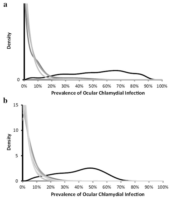
(a) Distribution of the prevalence of ocular chlamydia infection in 1-5 year-old children in 24 communities in the TEF study, Gurage, Ethiopia. (Lakew et al., 2009a) Communities were treated biannually with mass oral azithromycin. The distribution of infection for each cross-sectional survey is displayed as a density plot, in which each community’s contribution is the Bayesian posterior derived from the observed prevalence and a non-informative, uniform prior. The prevalence clearly decreases from baseline (black curve) to post-treatment visits at 12, 18, and 24 months (progressively lighter grey curves). (b) Distribution of the prevalence of ocular chlamydia infection in 0–9 year-old children in 24 communities in the TANA study, Amhara, Ethiopia. (Gebre et al., 2012) Communities were treated annually or biannually. The prevalence decreases from baseline (black curve) to post-treatment visits at 18, 24, 30, and 36 months (progressively lighter grey curves).
Data were from studies registered with ClinicalTrials.gov (NCT00221364 and NCT00322972) and approved by the National Ethics Review Committee of the Ethiopian Science and Technology Agency and the UCSF IRB (10-02630 and 10-02576).
2.1. Role of the funding source
The sponsors of the study had no role in trial design, data collection, data analysis, data interpretation, or writing of the report. TL had full access to all the data in the study and had final responsibility for the decision to submit for publication.
3. Results
Visits from the two studies were included if communities had received at least two mass antibiotic distributions and if the infection was documented to have decreased from 12 months earlier were included. The 2 and 6 month visits from TEF and the 6 and 12 month visits from TANA were excluded because they were after a single treatment. The post-treatment mean prevalence of infection in the two studies varied from 1.5% to 10.9% (Table 1), decreasing after mass treatment. Density plots of the community-level prevalence over time are displayed in Fig. 1. In TANA, where GPS was available, we were unable to demonstrate statistically significant geographical clustering for any post-treatment visit (Moran’s I: P = 0.32 for 18 months, P = 0.30 for 24 months, P = 0.14 for 30 months, P = 0.64 for 36 months).
We determined the parameter values which maximized the likelihood of obtaining the observed data for the 7 distributions: geometric, binomial, Poisson, discrete Weibull, negative binomial, beta binomial, zero-inflated geometric, and zero-inflated Poisson distributions (Table 2). In each case, the geometric distribution had the lowest (best) AICc. The binomial and Poisson distributions were the other single parameter distributions tested and offered far lower (worse) likelihoods. Note that the geometric distribution is a special case of the two-parameter distributions: discrete Weibull, negative binomial, and beta binomial (at least asymptotically), and the zero-inflated geometric distributions; thus with appropriate parameter choices, each can mimic a geometric distribution and achieve a likelihood of the observed data as least as high as that found with the geometric (with the exception of the zero-inflated geometric since we chose to use a single geometric scale parameter for each cross-sectional survey in a study, allowing the proportion that were zero to vary at each time point). Since none of these two-parameter distributions offered a significantly better fit than the geometric, the AICc was larger for these distributions. This suggests that these two-parameter distributions are less parsimonious than the geometric. The 95% confidence intervals for the estimation of the shape parameters for these two-parameter distributions included one, which in these parameterizations were consistent with the geometric (Table 2). Note that when we treated each individual cross-sectional survey separately allowing the shape parameter to vary with each visit, either the geometric or the zero-inflated geometric had the best AICc (for individual TANA visits, see Appendix B); the 95% CIs of shape parameter of the other three 2-parameter distributions included one for each separate visit. If the community-level prevalence of infection were indeed from a geometric distribution, how often would we have found results as close to a geometric as observed? With goodness-of-fit testing, we were unable to reject the hypothesis that the observed data from each entire study, or from any single post-treatment visit within a study, came from a geometric distribution (Table 1).
Table 2.
Model fit of the distribution of the community-level prevalence of infection in Ethiopian trachoma studies.
| TEF 12, 18, and 24 months | Shape parameter | No. of parameters | Loge Likelihood | AICc |
|---|---|---|---|---|
| Geometric | 4 | −125.79 | 263.576 | |
| Negative binomial | 0.824 (0.364 to 1.663) | 5 | −125.58 | 265.165 |
| Beta binomial | 0.742 (0.335 to 1.526) | 5 | −125.76 | 265.528 |
| Discrete Weibull | 0.999 (0.750 to 1.289) | 5 | −125.79 | 265.580 |
| Zero-inflated Geometric | 0.956 (0.934 to 0.972) | 5 | −130.91 | 275.815 |
| Poisson | 4 | −153.42 | 318.838 | |
| Binomial | 4 | −157.68 | 327.356 | |
| TANA 18, 24, 30, and 36 months | Shape parameter | No. of parameters | Loge Likelihood | AICc |
| Geometric | 5 | −157.544 | 329.089 | |
| Beta binomial | 0.926 (0.674 to 1.412) | 6 | −157.435 | 330.871 |
| Negative binomial | 0.960 (0.462 to 1.820) | 6 | −157.535 | 331.070 |
| Zero-inflated Geometric | 0.957 (0.935 to 0.976) | 6 | −157.894 | 331.788 |
| Discrete Weibull | 1.030 (0.792 to 1.363) | 6 | −158.390 | 332.779 |
| Poisson | 5 | −179.668 | 373.335 | |
| Binomial | 5 | −181.924 | 377.849 |
Table 1.
Prevalence of ocular chlamydial infection in longitudinal studies of trachoma in Ethiopia.
| Prevalence of Infection
|
||||
|---|---|---|---|---|
| Communities | Mean prevalence | Standard deviation of prevalence | Geometric distribution goodness of fit test (P-value) | |
| TEF Ethiopia | ||||
| 0 Months | 16 | 0.529 | 0.218 | 0.03 |
| 12 Months | 16 | 0.069 | 0.109 | 0.23 |
| 18 Months | 16 | 0.032 | 0.037 | 0.58 |
| 24 Months | 16 | 0.020 | 0.022 | 0.30 |
| TANA Ethiopia | ||||
| 0 Months | 24 | 0.394 | 0.153 | 0.03 |
| 18 Months | 24 | 0.043 | 0.050 | 0.29 |
| 24 Months | 24 | 0.036 | 0.041 | 0.12 |
| 30 Months | 24 | 0.015 | 0.025 | 0.89 |
| 36 Months | 24 | 0.026 | 0.037 | 0.74 |
As sensitivity analyses, simulations of an SIS model with mass action and R0 = 0.5 were used to construct a dataset similar to the Ethiopian data with 24 communities evaluated at 4 different time points. The geometric offered the optimal AICc, and in no case did the addition of a second parameter result in a statistically superior fit (likelihood ratio test, P > 0.05). Similar sized sets of communities simulated from discrete Weibull distributions with shape parameters of 0.5 and 2.0 were easily distinguishable from the geometric (P < 0.05), with the Weibull distribution having the optimal AICc. The model selection process correctly identified samples taken from discrete Weibull distributions with shape parameters 0.5 and 2.0. Empirical, pre-treatment surveys from the two Ethiopian areas studied were not consistent with a geometric distribution (Table 2). Simulations of an SIS model with mass action and R0 = 1.0, 1.5, and 2.0 (without treatment) were used to construct datasets similar to the Ethiopian data with 24 communities evaluated at 4 different time points. In all cases, the Poisson and the binomial distribution each had a far lower (better) AICc than the geometric distribution. Similar sets with an estimated treated reproduction number of Rt = 1.0, 1.5, and 2.0 also were better fit by the Poisson and binomial than the geometric (for Rt = 1.0 see Appendix C).
4. Discussion
When assessing whether an infectious disease is on its way to elimination, survey of infection in every community in a region over time may be infeasible due to the costs of collection and processing. However, if the community-level cross-sectional prevalence of infection in an area can be approximated by a geometric distribution, then a single cross-sectional sampling of communities can provide an accurate assessment of infection in an area. Here, we assessed two large, population-based surveys recently performed in multiple communities in controlled settings where transmission conditions were similar and constant, and where trachoma was known to be disappearing due to programmatic activity. In each case, the geometric distribution fitted the observed data better than the other distributions tested. Furthermore, we were unable to reject the hypothesis that each prevalence was drawn independently from a geometric distribution in these two settings where trachoma was known to be disappearing. Much of the distributional information available from examining every community is captured by the single, sufficient parameter of a geometric distribution.
Since a geometric distribution has a relatively heavy tail, outliers are to be expected. While we cannot discount the possibility that a high prevalence village has inherently higher transmission than its neighbors, this need not be hypothesized; occasional high prevalence communities are to be expected even from a set of communities with identically transmission characteristics, and do not necessarily reflect a hot spot for transmission or a program failure. Models predict that infection will still disappear from the high prevalence communities in the tail of this distribution (Ray et al., 2007, 2009). Empirical studies support this. Reports from Nepal, Tanzania, and the Gambia have found that the prevalence of infection in the most severely affected village in an otherwise hypo-endemic area decreases in the absence of treatment (Jha et al., 2002; Gaynor et al., 2003; Solomon et al., 2004; Burton et al., 2010). Longitudinal studies that focused on the most severely affected community in an area may have led researchers to interpret this regression to the mean as enhanced efficacy of antibiotics and other interventions, relative to studies which included a control group (Gebre et al., 2011; Gaynor et al., 2003; Solomon et al., 2004; Stoller et al., 2011; West et al., 2006).
Recent models fitted to data from areas moderately endemic for trachoma suggest the possibility of positive feedback (Lietman et al., 2011); that is, additional infection in a community may increase the per-susceptible risk of infection more than the proportional increase assumed by the mass-action model. In meso-endemic areas this may result in a bi-modal distribution of prevalence, with a peak at elimination, and a second peak around an endemic equilibrium (Lietman et al., 2011). Note though that even a positive (or negative) feedback model should behave as a mass-action SIS model at a low enough prevalence, and thus the geometric distribution would still be expected. We would expect a mixture of two distributions if a survey area included distinct areas of low and high transmission. If the unit of the survey was not a single community, but a cluster of communities, we would expect the convolution of several geometric distributions (i.e. a negative binomial distribution with a shape parameter greater than one).
There are many limitations of this study. These 2–4 years longitudinal studies show decrease in prevalence, but do not follow to complete elimination. The goodness-of-fit testing assumes independent sampling from an identical distribution; while the samples were exchangeable, there may be geographical correlations. None of the sentinel communities in either TEF or TANA were contiguous, and in TANA, where GPS was available, we were unable to demonstrate any significant geographical clustering. Note that any correlation would have made it more difficult to exclude a geometric distribution, hence in that sense our analysis was conservative. Likewise, the prevalence of infection in treatment arms in TANA was not significantly different; separation by treatment arm would have resulted in smaller datasets and more difficult exclusion of the geometric distribution.
The endgame for disease control offers special challenges. While districts or subdistricts may meet thresholds for control, concern for missing higher prevalence communities has led some to argue that programs need to examine every community. Knowledge that community-level prevalence approximates a geometric distribution, and that the scale of the distribution can be estimated from a survey sample, may allow programs the confidence they need to conserve resources. Population-based surveys of all communities in trachoma-endemic areas would be an enormous undertaking, and appears to be unnecessary. Programs can assess whether they are on track towards elimination by a single cross-sectional survey. If the distribution of the community prevalence of infection in a particular area is consistent with a geometric distribution, this may be a good sign, since this would not be expected in areas where infection is not disappearing (Nåsell, 1996; Lietman et al., 2011). Note that elimination would only be expected to eventually occur if conditions remain the same. An increase in transmission due to discontinuation of programmatic activity of deterioration of socioeconomic status could prevent elimination. Additional studies will be necessary to determine whether the prevalence of the clinical signs of infection on which programs rely so heavily can also be approximated by a geometric distribution.
Can trachoma be eradicated? The strains of chlamydia that cause the disease are only transmitted between humans. No vaccine has been shown efficacious. While the WHO recommends hygiene and latrine programs, no non-antibiotic measure has yet been proven to decrease infection (Emerson et al., 2000; Stoller et al., 2011). Mass antibiotics distributions have proven effective in cluster-randomized trials, and have so far been well tolerated (Schachter et al., 1999; Chidambaram et al., 2006; House et al., 2009). Trachoma has been disappearing in some areas, even in the absence of a dedicated trachoma program (Hoechsmann et al., 2001; Jha et al., 2002; Dolin et al., 1997). This report suggests that if efforts are continued, infection will eventually disappear in previously hyper-endemic areas of Ethiopia. If these are representative of other severely affected regions, if trachoma programs can be maintained, and if antibiotic resistance does not evolve, then global eradication of trachoma may indeed be feasible.
Acknowledgments
This work was supported by NIH U10 EY016214, NIH GM 087728 (MIDAS), the Harper-Inglis Trust, That Man May See, and Research to Prevent Blindness.
Appendix A
The discrete distributions were parameterized such that the prevalence of infection would not, on average, be affected by that community’s population size; the scale parameter which was maximized was the probability of an individual being infected at that cross-sectional survey, in that study. The 2-parameter distributions, were parameterized such that the shape parameter would be the same for all visits, and would equal one when the distribution represented a geometric distribution (asymptotically in the case of the beta binomial distribution). The probability mass functions used are:
Geometric distribution:
Poisson distribution:
Binomial distribution:
Discrete Weibull distribution:
Negative Binomial distribution:
Beta Binomial distribution:
Zero-inflated Geometric distribution:
Zero-inflated Poisson distribution: where α is the reparameterized shape parameter, t is the time point, j is the community, pt is the mean prevalence of the distribution for the time point t, nj is the number of individuals in the jth community, and i is the number infected in the community. For the two zero-inflated distributions, we allowed the shape parameter to vary between visits, keeping the prevalence parameter constant.
Appendix B
Model fitting for individual visits of TANA, ranked by AICc of models for that visit. The best-fit shape and scale parameters are included.
| Visit | AICc | Distribution | Parameters | logLikelihood | Shape | Scale |
|---|---|---|---|---|---|---|
| TANA baseline | 173.55 | Negative Binomial | 5 | –80.107 | 8.352 | 0.395 |
| 187.12 | Discrete Weibull | 5 | –86.894 | 1.345 | 1.000 | |
| 190.30 | Poisson | 4 | –90.097 | 0.397 | ||
| 193.53 | Zero-inflated Poisson | 5 | –90.097 | 0.397 | 0.000 | |
| 193.72 | Geometric | 4 | –91.809 | 0.395 | ||
| 196.95 | Zero-inflated Geometric | 5 | –91.809 | 0.395 | 0.000 | |
| 218.73 | Binomial | 4 | –104.314 | 0.397 | ||
| TANA 18 months | 105.21 | Geometric | 4 | –47.551 | 0.043 | |
| 108.16 | Discrete Weibull | 5 | –47.411 | 1.101 | 0.051 | |
| 108.19 | Negative Binomial | 5 | –47.429 | 1.270 | 0.043 | |
| 108.44 | Zero-inflated Geometric | 5 | –47.551 | 0.043 | 0.000 | |
| 117.63 | Zero-inflated Poisson | 5 | –52.150 | 0.054 | 0.204 | |
| 120.70 | Poisson | 4 | –55.297 | 0.043 | ||
| 122.78 | Binomial | 4 | –56.338 | 0.043 | ||
| TANA 24 months | 96.71 | Geometric | 4 | –43.304 | 0.036 | |
| 99.48 | Zero-inflated Poisson | 5 | –43.071 | 0.053 | 0.327 | |
| 99.84 | Discrete Weibull | 5 | –43.256 | 1.066 | 0.040 | |
| 99.87 | Negative Binomial | 5 | –43.270 | 1.160 | 0.036 | |
| 99.91 | Zero-inflated Geometric | 5 | –43.287 | 0.037 | 0.034 | |
| 106.46 | Poisson | 4 | –48.179 | 0.036 | ||
| 107.53 | Binomial | 4 | –48.711 | 0.036 | ||
| TANA 30 months | 67.88 | Geometric | 4 | –28.885 | 0.015 | |
| 69.92 | Zero-inflated Poisson | 5 | –28.294 | 0.032 | 0.529 | |
| 70.40 | Zero-inflated Geometric | 5 | –28.532 | 0.020 | 0.257 | |
| 70.66 | Negative Binomial | 5 | –28.663 | 0.590 | 0.015 | |
| 70.72 | Discrete Weibull | 5 | –28.695 | 0.855 | 0.013 | |
| 73.47 | Poisson | 4 | –31.681 | 0.015 | ||
| 73.80 | 4 | –31.847 | 0.015 | |||
| TANA 36 months | 85.71 | Geometric | 4 | –37.804 | 0.026 | |
| 88.33 | Zero-inflated Geometric | 5 | –37.499 | 0.032 | 0.173 | |
| 88.39 | Discrete Weibull | 5 | –37.530 | 0.853 | 0.021 | |
| 88.41 | Negative Binomial | 5 | –37.539 | 0.655 | 0.026 | |
| 90.82 | Zero-inflated Poisson | 5 | –38.745 | 0.047 | 0.440 | |
| 99.13 | Poisson | 4 | –44.511 | 0.027 | ||
| 100.16 | Binomial | 4 | –45.028 | 0.027 |
Appendix C
Model fitting for individual visits of simulated SIS model, ranked by AICc of models for that visit. The best-fit shape and scale parameters are included. Parameters for the model include: population of 50 children per community, R0 = 2.6 (in the absence of treatment), estimated Rt = 1.0 (in the presence of treatment)(Melese et al., 2004), 80% coverage with 100% effective antibiotic, rate of recovery 1/52 weeks.
| Visit | AICc | Distribution | Parameters | Log Likelihood | Shape | Scale |
|---|---|---|---|---|---|---|
| Simulated baseline | 148.55 | Poisson | 1 | −73.183 | 0.395 | |
| 150.94 | Zero-inflated Poisson | 2 | −73.183 | 0.572 | 1.000 | |
| 150.94 | Negative Binomial | 2 | −73.183 | 1120,000 | 0.397 | |
| 159.10 | Binomial | 1 | −78.462 | 0.000 | ||
| 206.20 | Discrete Weibull | 2 | −100.814 | 1.223 | 0.395 | |
| 212.02 | Geometric | 1 | −104.917 | 0.000 | ||
| 214.41 | Zero-inflated Geometric | 2 | −104.917 | 0.573 | 0.397 | |
| Simulated 18 months | 151.41 | Negative Binomial | 2 | −73.419 | 4.261 | 0.043 |
| 151.66 | Discrete Weibull | 2 | −73.546 | 1.669 | 0.051 | |
| 160.52 | Zero-inflated Poisson | 2 | −77.972 | 0.197 | 0.043 | |
| 160.49 | Geometric | 1 | −79.152 | 0.000 | ||
| 162.87 | Zero-inflated Geometric | 2 | −79.152 | 0.189 | 0.204 | |
| 169.14 | Poisson | 1 | −83.477 | 0.043 | ||
| 179.79 | Binomial | 1 | −88.804 | 0.043 | ||
| Simulated 24 months | 165.43 | Negative Binomial | 2 | −80.429 | 3.944 | 0.036 |
| 167.17 | Discrete Weibull | 2 | −81.297 | 1.506 | 0.327 | |
| 174.50 | Geometric | 1 | −86.161 | 0.040 | ||
| 176.89 | Zero-inflated Geometric | 2 | −86.161 | 0.257 | 0.036 | |
| 182.11 | Zero-inflated Poisson | 2 | −88.769 | 0.268 | 0.034 | |
| 197.62 | Poisson | 1 | −97.720 | 0.036 | ||
| 222.16 | Binomial | 1 | −109.989 | 0.036 | ||
| Simulated 30 months | 174.68 | Negative Binomial | 2 | −85.053 | 4.651 | 0.015 |
| 179.35 | Discrete Weibull | 2 | −87.390 | 1.401 | 0.529 | |
| 185.06 | Zero-inflated Poisson | 2 | −90.243 | 0.345 | 0.257 | |
| 186.29 | Geometric | 1 | −92.052 | 0.015 | ||
| 188.68 | Zero-inflated Geometric | 2 | −92.052 | 0.331 | 0.013 | |
| 208.15 | Poisson | 1 | −102.983 | 0.015 | ||
| 241.48 | Binomial | 1 | −119.651 | 0.015 | ||
| Simulated 36 months | 111.89 | Discrete Weibull | 2 | −53.662 | 1.802 | 0.026 |
| 112.17 | Negative Binomial | 2 | −53.799 | 5.766 | 0.173 | |
| 112.64 | Zero-inflated Poisson | 2 | −54.033 | 0.078 | 0.021 | |
| 112.64 | Poisson | 1 | −55.229 | 0.026 | ||
| 113.73 | Binomial | 1 | −55.775 | 0.440 | ||
| 118.57 | Geometric | 1 | −58.193 | 0.027 | ||
| 120.96 | Zero-inflated Geometric | 2 | −58.193 | 0.073 | 0.027 |
References
- Resnikoff S, Pascolini D, Etya’ale D, Kocur I, Pararajasegaram R, et al. Global data on visual impairment in the year 2002. Bull World Health Organ. 2004;82:844–851. [PMC free article] [PubMed] [Google Scholar]
- Schachter J, West SK, Mabey D, Dawson CR, Bobo L, et al. Azithromycin in control of trachoma. Lancet. 1999;354:630–635. doi: 10.1016/S0140-6736(98)12387-5. [DOI] [PubMed] [Google Scholar]
- Chidambaram JD, Alemayehu W, Melese M, Lakew T, Yi E, et al. Effect of a single mass antibiotic distribution on the prevalence of infectious trachoma. JAMA. 2006;295:1142–1146. doi: 10.1001/jama.295.10.1142. [DOI] [PubMed] [Google Scholar]
- House JI, Ayele B, Porco TC, Zhou Z, Hong KC, et al. Assessment of herd protection against trachoma due to repeated mass antibiotic distributions: a cluster-randomised trial. Lancet. 2009;373:1111–1118. doi: 10.1016/S0140-6736(09)60323-8. [DOI] [PubMed] [Google Scholar]
- Lietman T, Porco T, Dawson C, Blower S. Global elimination of trachoma: how frequently should we administer mass chemotherapy? Nat Med. 1999;5:572–576. doi: 10.1038/8451. [DOI] [PubMed] [Google Scholar]
- Gebre T, Ayele B, Zerihun M, Genet A, Stoller NE, et al. Comparison of annual versus twice-yearly mass azithromycin treatment for hyperendemic trachoma in Ethiopia: a cluster-randomised trial. Lancet. 2012;379(9811):143–151. doi: 10.1016/S0140-6736(11)61515-8. [DOI] [PubMed] [Google Scholar]
- Emerson PM, Cairncross S, Bailey RL, Mabey DC. Review of the evidence base for the ‘F’ and ‘E’ components of the SAFE strategy for trachoma control. Trop Med Int Health. 2000;5:515–527. doi: 10.1046/j.1365-3156.2000.00603.x. [DOI] [PubMed] [Google Scholar]
- Dolin PJ, Faal H, Johnson GJ, Ajewole J, Mohamed AA, et al. Trachoma in The Gambia. Br J Ophthalmol. 1998;82:930–933. doi: 10.1136/bjo.82.8.930. [DOI] [PMC free article] [PubMed] [Google Scholar]
- Hoechsmann A, Metcalfe N, Kanjaloti S, Godia H, Mtambo O, et al. Reduction of trachoma in the absence of antibiotic treatment: evidence from a population-based survey in Malawi. Ophthalmic Epidemiol. 2001;8:145–153. doi: 10.1076/opep.8.2.145.4169. [DOI] [PubMed] [Google Scholar]
- Jha H, Chaudary J, Bhatta R, Miao Y, Osaki-Holm S, et al. Disappearance of trachoma in western Nepal. Clin Infect Dis. 2002;35:765–768. doi: 10.1086/342298. [DOI] [PubMed] [Google Scholar]
- Brauer F, van den Driessche P, Wu J. In: Mathematical epidemiology. Maini PK, editor. Springer-Verlag; Berlin: 2008. [Google Scholar]
- Cavender JA. Quasi-staionary distributions of birth-and-death processes. Adv Appl Probab. 1978;10:570–586. [Google Scholar]
- Nåsell I. On the quasi-stationary distribution of the stochastic logistic epidemic. Math Biosci. 1999;156:21–40. doi: 10.1016/s0025-5564(98)10059-7. [DOI] [PubMed] [Google Scholar]
- Nåsell I. The quasi-stationary distribution of the closed endemic SIS MODEL. Adv Appl Probab. 1996;28:895–932. [Google Scholar]
- Ray KJ, Porco TC, Hong KC, Lee DC, Alemayehu W, et al. A rationale for continuing mass antibiotic distributions for trachoma. BMC Infect Dis. 2007;7:91. doi: 10.1186/1471-2334-7-91. [DOI] [PMC free article] [PubMed] [Google Scholar]
- Blake IM, Burton MJ, Bailey RL, Solomon AW, West S, et al. Estimating household and community transmission of ocular Chlamydia trachomatis. PLoS Negl Trop Dis. 2009;3:e401. doi: 10.1371/journal.pntd.0000401. [DOI] [PMC free article] [PubMed] [Google Scholar]
- Ray KJ, Lietman TM, Porco TC, Keenan JD, Bailey RL, et al. When can antibiotic treatments for trachoma be discontinued? Graduating communities in three African countries. PLoS Negl Trop Dis. 2009;3:e458. doi: 10.1371/journal.pntd.0000458. [DOI] [PMC free article] [PubMed] [Google Scholar]
- Holm SO, Jha HC, Bhatta RC, Chaudhary JS, Thapa BB, et al. Comparison of two azithromycin distribution strategies for controlling trachoma in Nepal. Bull World Health Organ. 2001;79:194–200. [PMC free article] [PubMed] [Google Scholar]
- Lakew T, House J, Hong KC, Yi E, Alemayehu W, et al. Reduction and return of infectious trachoma in severely affected communities in Ethiopia. PLoS Negl Trop Dis. 2009a;3:e376. doi: 10.1371/journal.pntd.0000376. [DOI] [PMC free article] [PubMed] [Google Scholar]
- Porco TC, Gebre T, Ayele B, House J, Keenan J, et al. Effect of mass distribution of azithromycin for trachoma control on overall mortality in Ethiopian children: a randomized trial. JAMA. 2009;302:962–968. doi: 10.1001/jama.2009.1266. [DOI] [PubMed] [Google Scholar]
- Gebre T, Ayele B, Zerihun M, Genet A, Stoller NE, et al. Comparison of annual versus twice-yearly mass azithromycin treatment for hyperendemic trachoma in Ethiopia: a cluster-randomised trial. Lancet. 2012;379:143–151. doi: 10.1016/S0140-6736(11)61515-8. [DOI] [PubMed] [Google Scholar]
- Lakew T, Alemayehu W, Melese M, Yi E, House JI, et al. Importance of coverage and endemicity on the return of infectious trachoma after a single mass antibiotic distribution. PLoS Negl Trop Dis. 2009b;3:e507. doi: 10.1371/journal.pntd.0000507. [DOI] [PMC free article] [PubMed] [Google Scholar]
- Johnson NL, Kotz S, Kepm AW. In: univariate discrete distributions. Barnett V, Bradley RA, Fisher NI, Hunter JS, Kadane JB, et al., editors. John Wiley & Sons, Inc; New York, NY: 1993. [Google Scholar]
- Burnham KP, Anderson DR. Model selection and inference: A practical information-theoretic approach. New York, NY: Springer; 1998. [Google Scholar]
- Lietman TM, Gebre T, Ayele B, Ray KJ, Maher MC, et al. The epidemi-ological dynamics of infectious trachoma may facilitate elimination. Epidemics. 2011;3:119–124. doi: 10.1016/j.epidem.2011.03.004. [DOI] [PMC free article] [PubMed] [Google Scholar]
- Gaynor BD, Miao Y, Cevallos V, Jha H, Chaudary JS, et al. Eliminating trachoma in areas with limited disease. Emerg Infect Dis. 2003;9:596–598. doi: 10.3201/eid0905.020577. [DOI] [PMC free article] [PubMed] [Google Scholar]
- Solomon AW, Holland MJ, Alexander ND, Massae PA, Aguirre A, et al. Mass treatment with single-dose azithromycin for trachoma. N Engl J Med. 2004;351:1962–1971. doi: 10.1056/NEJMoa040979. [DOI] [PMC free article] [PubMed] [Google Scholar]
- Burton MJ, Holland MJ, Makalo P, Aryee EA, Sillah A, et al. Profound and sustained reduction in Chlamydia trachomatis in The Gambia: a five-year longitudinal study of trachoma endemic communities. PLoS Negl Trop Dis. 2010;4 doi: 10.1371/journal.pntd.0000835. [DOI] [PMC free article] [PubMed] [Google Scholar]
- Stoller NE, Gebre T, Ayele B, Zerihun M, Assefa Y, et al. Efficacy of latrine promotion on emergence of infection with ocular Chlamydia trachomatis after mass antibiotic treatment: a cluster-randomized trial. Int Health. 2011;3:75–84. doi: 10.1016/j.inhe.2011.03.004. [DOI] [PMC free article] [PubMed] [Google Scholar]
- West SK, Emerson PM, Mkocha H, McHiwa W, Munoz B, et al. Intensive insecticide spraying for fly control after mass antibiotic treatment for trachoma in a hyperendemic setting: a randomised trial. Lancet. 2006;368:596–600. doi: 10.1016/S0140-6736(06)69203-9. [DOI] [PubMed] [Google Scholar]
- Dolin PJ, Faal H, Johnson GJ, Minassian D, Sowa S, et al. Reduction of trachoma in a sub-Saharan village in absence of a disease control programme. Lancet. 1997;349:1511–1512. doi: 10.1016/s0140-6736(97)01355-x. [DOI] [PubMed] [Google Scholar]
- Melese M, Chidambaram JD, Alemayehu W, Lee DC, Yi EH, et al. Feasibility of eliminating ocular Chlamydia trachomatis with repeat mass antibiotic treatments. JAMA. 2004;292:721–725. doi: 10.1001/jama.292.6.721. [DOI] [PubMed] [Google Scholar]