The role of fine-grained annotations in supervised recognition of risk factors for heart disease from EHRs

Abstract

This paper describes a supervised machine learning approach for identifying heart disease risk factors in clinical text, and assessing the impact of annotation granularity and quality on the system's ability to recognize these risk factors. We utilize a series of support vector machine models in conjunction with manually built lexicons to classify triggers specific to each risk factor. The features used for classification were quite simple, utilizing only lexical information and ignoring higher-level linguistic information such as syntax and semantics. Instead, we incorporated high-quality data to train the models by annotating additional information on top of a standard corpus. Despite the relative simplicity of the system, it achieves the highest scores (micro- and macro-F₁, and micro- and macro-recall) out of the 20 participants in the 2014 i2b2/UTHealth Shared Task. This system obtains a micro- (macro-) precision of 0.8951 (0.8965), recall of 0.9625 (0.9611), and F₁-measure of 0.9276 (0.9277). Additionally, we perform a series of experiments to assess the value of the annotated data we created. These experiments show how manually-labeled negative annotations can improve information extraction performance, demonstrating the importance of high-quality, fine-grained natural language annotations.

1 Introduction

A significant amount of a patient's medical information in an electronic health record (EHR) is stored in unstructured text. Natural language processing (NLP) techniques are therefore necessary to extract critical medical information to improve patient care. For most serious conditions, many types of relevant information (e.g., diagnoses, lab results, medications) need to be extracted from the patient's records, often over a length of time that spans several narrative notes. The 2014 i2b2/UTHealth Shared Task Track 2 (hereafter, “the 2014 i2b2 task”) [1] evaluates such a case by focusing on the many risk factors for heart disease, including comorbidities, laboratory tests, medications, and family history, with over 30 specific risk factors. This article describes the method utilized by the U.S. National Library of Medicine (NLM) for the 2014 i2b2 task. Our method is a supervised machine learning (ML) approach that finished first overall in the task, including both the highest (micro and macro) recall and (micro and macro) F₁-measure.

Most state-of-the-art NLP methods for extracting information from EHRs utilize supervised ML techniques [2, 3, 4]. However, one important yet understudied issue in developing ML-based NLP systems for EHRs is the impact of the granularity of the labeled data. To assess the impact of granularity, we evaluate a relatively simple information extraction (IE) system on two sets of labels derived from the 2014 i2b2 task corpus: (a) coarse-grained document-level annotations with at least one positive mention-level support span, and (b) fine-grained mention-level annotations where every relevant supporting span is marked as positive or negative. The labels from (a) were provided by the task organizers, and are described in the Task Description section below. The labels from (b) were created by NLM staff as part of our participation in the 2014 i2b2 task. The system utilizing this fine-grained data achieved the highest score among the 20 participants. Further, unlike most of the other top-performing participants, the system was entirely limited to lexical information: no syntactic information (e.g., parts-of-speech, dependencies) or semantic information (e.g., word senses, semantic roles, named entities) was utilized. Instead, our primary contribution was demonstrating the importance of fine-grained mention-level annotations for developing supervised ML methods for clinical NLP. In this article, we describe the data provided by the organizers, the data annotated by NLM, the supervised ML system for extracting risk factors, and the results on the 2014 i2b2 task. Additionally, we describe post-hoc experiments to evaluate how this system would have performed without the fine-grained annotated data.

2 Background

Since a significant amount of EHR information can be stored in an unstructured narrative, the range of NLP tasks spans almost the full range of potential EHR support functions [5]. The foundation for NLP-based applications is based on information extraction (IE), the task of automatically converting some particular type of unstructured text into a structured form. Widely used IE systems include MetaMap [6], MedLEE [7], and cTAKES [8]. To supplement these, the negation algorithm NegEx [9], and its successor method for more general context detection, ConText [10], are commonly used to understand negation and modality. Due to the difficulty in sharing clinical data, several de-identified corpora have been created, often in coordination with a shared task, to allow researchers to compare IE methods on a common dataset. Such shared tasks include the i2b2 shared tasks, discussed below, as well as the recent ShARe/CLEF eHealth task [11], which evaluated concept extraction and normalization.

There have been seven i2b2 challenges to date, each dealing with at least one clinical IE task and evaluating participants on a de-identified clinical dataset. The tasks have dealt with de-identification and smoking detection in 2006 [12, 13]; obesity detection in 2008 [14]; medication extraction in 2009 [15]; concept extraction, assertion classification, and relation identification in 2010 [2]; co-reference [3] and sentiment analysis [16] in 2011; event extraction, temporal expression extraction, and temporal relation identification in 2012 [4]; and, most recently, de-identification and heart disease risk factor identification in 2014 [1]. The heart disease risk factor identification task, which is the focus of the article, contains elements of many of the previous tasks: (i) many of the risk factors are expressed as concepts/events similar to the 2010 and 2012 tasks; (ii) smoking (2006), obesity (2008), and medications (2009) are among those risk factors, (iii) negation and modality play an important role in determining whether a concept is identified as a risk factor (2010 and 2012); and (iv) the temporal aspect (2012) of each risk factor must be identified to qualify the patient's risk of heart disease.

While no previous task has focused on the exact same set of risk factors as the 2014 i2b2 task, most of the individual risk factors have been studied in previous work. For example, Cimino et al. [17] and Gold et al. [18] perform medication extraction from clinical notes. Goryachev et al. [19], Lewis et al. [20], and Friedlin & McDonald [21] all extract family history information. Finally, a significant amount of research has focused on extracting temporal information from clinical narratives [22, 23, 24], as temporality is a crucial element to medical reasoning.

3 Task Description

The 2014 i2b2/UTHealth Shared Task Track 2 evaluates a system's ability to determine whether a patient has particular heart disease risk factors based on his or her unstructured, longitudinal medical records. The track evaluates 36 individual risk factors (18 if all medication types are considered collectively) in eight general categories:

1. Diabetes risk factors: diabetes mention, high A1c (over 6.5), high glucose (two measurements over 126)

2. Coronary artery disease (CAD) risk factors: CAD mention, CAD event (e.g., MI, STEMI, cardiac arrest), CAD test result (showing ischemia or coronary stenoses), CAD symptom (chest pain consistent with angina)

3. Hyperlipidemia risk factors: hyperlipidemia/hypercholesterolemia mention, high cholesterol (over 240), high LDL (over 100)

4. Hypertension risk factors: hypertension mention, high blood pressure (systolic over 140 or diastolic over 90)

5. Obesity risk factors: obese mention, high BMI (over 30), high waist circumference (over 40 inches in men or 35 inches in women)

6. Family history risk factor: mention of immediate family member with history of early CAD

7. Smoking risk factor: whether patient currently smokes (current), smoked in the distant past (past), smoked at some unspecified point (ever), never smoked (never), or unknown (unknown)

8. Medication risk factors: whether the patient takes any medications indicative of the above risk factors. This includes the following drugs and drug classes: ACE inhibitor, amylin, anti-diabetes, ARB, aspirin, beta blocker, calcium channel blocker, diuretic, DPP4 inhibitor, ezetimibe, fibrate, insulin, metformin, niacin, nitrate, statin, sulfonylurea, thiazolidinedione, thienopyridine

Here, a mention is a statement of a specific disease diagnosis (e.g., “patient has diabetes”) instead of a diagnosis based on a measurement (e.g., “A1c is 8.5”) or other factor, and is limited to the patient (as opposed to a family member).

The organizers provided 790 training notes and 514 testing notes. Between 2 and 5 notes were provided for each patient to enable longitudinal analysis, though the manual annotations were done at the document level without considering previous notes (so, for instance, an early note might be positive for diabetes while a later note is marked as negative if it does not contain an explicit diabetes diagnosis). Each note contained 617 words on average. Each of the risk factors above is annotated at the document level (e.g., whether a note contains a high A1c value) by asking annotators to highlight at least one text span that indicates the risk factor (e.g., “A1c of 7.1”), additionally labeling the time of the risk factor (before, during, or after the hospital visit, or any combination of these). These text spans were provided by the organizers in addition to the document-level decision. However, since this is a document-level task, annotators were not provided with guidelines to ensure consistent span annotation. If two of three annotators found some support for a risk factor (and agreed on the time), the note was considered positive for that risk factor (and time) and all the highlighted spans were included in the annotations. No inter-annotator conflict resolution was performed. Further, when only one annotator found a textual support, the document was considered negative and those highlighted spans were not included in the annotations. Also, when annotators agreed on a risk factor but disagreed on its time, the document was also considered negative. See Stubbs et al. [25] for more details on the risk factor annotation process. The organizers' annotation decisions were made to increase the total number of annotated notes: a choice of quantity over both quality (since no resolution was performed) and granularity (document-level instead of mention-level). However, this has important ramifications on the types of automatic methods usable for the task. Since supervised ML methods require both positive and negative examples, and the only negative examples were at the document level and not mention level, any mention-level ML method, such as the one described in this article, either needs additional labels or must rely on heuristics to automatically label negative examples.

4 NLM Annotations

To address the shortcomings of the original data described in the Task Description section, our annotation process had five goals:

1. Achievable annotation time

2. Consistent annotation boundaries

3. Both positive and negative annotations

4. Classification of types of negative annotations

5. Maximum number of annotations per document

One of the most time-consuming and least productive requirements of annotation is reading through irrelevant parts of a patient's record. Yet, if they read too quickly, annotators may miss crucial information. We thus utilized a form of pre-annotation of candidate risk factors that leverages the data provided by the organizers. Based on the spans highlighted by the original annotators, we created a lexicon for each risk factor.

The lexicon was manually built to ensure a set of consistent, maximal annotation boundaries. Since IE classifiers utilize linguistic cues, it is important that span boundaries are expanded to best recognize these contextual elements. For example, if the word before a lexicon match is no, that provides useful information that the risk factor is negated. If our lexicon only contained the word diabetes, this cue would work well for the phrase “no diabetes”, but not for “no type 2 diabetes”. Our annotations, therefore, should span the full extent of the risk factor. The lexicons were further expanded based on known synonyms that were missing in the set of spans highlighted by the original annotators.

The boundaries of the original highlighted spans were adjusted to match the terms in the lexicons, while some incorrect annotations were removed. The adjusted spans were then automatically labeled as positive and thus did not need to be addressed by the NLM annotators (about one-third of the total lexicon matches). The remaining lexicon matches were then pre-annotated so that the NLM annotators did not need to read the full notes, only the immediate context of each risk factor annotation to determine whether it was positive/negative and, if possible, what temporal classification should be assigned. This also ensured annotators were able to easily label every mention of a risk factor in the notes, maximizing the number of examples for training. For measurements (A1c, glucose, cholesterol, LDL, blood pressure, BMI), the lexicon contained the name of the measurement (the “base”), and the right context was searched for numbers that were within the valid range for the given lab test. We annotated all measurements, not simply those above the threshold. Since the values under the threshold could easily be filtered automatically, all actual measurement values were considered positive. This increased the number of available annotations while also allowing the threshold to be changed at a later time without altering the annotations.

Negative concepts are split into two cases: validity and polarity. While a negative polarity corresponds to the linguistic notion of negation (e.g., “patient is not obese”, “goal A1c is 7.0”), a negative validity corresponds to a lexicon match that does not refer to the actual concept. Invalid concepts were typically the result of word sense differences. Usually this was either abbreviations that in the given context were referring to something else, or a measurement whose value span is not actually a valid measurement (e.g., in the phrase “A1c 7.8 19 days ago”, the value 7.8 is positive, while the value 19 is invalid). By classifying whether negative risk factors are either negations or invalid, classifiers can focus on separate linguistic problems, such as negation and word sense disambiguation.

Only two-thirds of the training data was annotated in this way, as the final third was only available a few days before the submission deadline. Four annotators, including three MDs (LR, SA, DDF) and one medical librarian (SS), double-annotated the documents one risk factor at a time. The annotators worked in fixed pairs, with disagreements being resolved first within each annotator pair, then with an annotator from the other pair acting as tie-breaker as needed. Both pairs annotated all of the risk factors (one annotating the even-numbered documents, the other the odd-numbered), with the exception of CAD events, test results, and symptoms, which were entirely annotated by one pair due to time availability.

Table 1 shows a comparison of the original and NLM annotations at the document level. For instance, the original set had 1,560 Diabetes mention annotations, while the NLM annotators added a further 22 annotations without removing any. While many mention-level annotations were pruned (e.g., a medication being marked as a CAD mention), few of the original annotations at the document level were removed. A notable exception was Obese mentions, where 12 annotations were removed that referred to obesity of the abdomen. The lexicon-based method allowed for finding many additional mention-level annotations, which resulted in a significant number of document-level changes. Notably, the number of document-level Glucose and Cholesterol annotations were significantly increased (though this is before the minimum two glucose measurement criteria is applied, so the final count would be smaller). In total, 33 document-level annotations were removed, while 1,178 document-level annotations were added.

Table 1.

Annotation differences between the original and NLM sets. Counts are by document and time, not mention. The maximum count for most annotation types is three times the number of documents (i.e., an annotation for before DCT, during DCT, and after DCT in each note). Medications, however, can have up to 57 annotations per note (for the 19 types of medication).

Annotation	Original Only	Both	NLM Only
Diabetes Mention	0	1560	22
A1C	3	107	44
Glucose	0	25	187
CAD Mention	3	777	19
CAD Event	0	246	26
CAD Test Result	2	77	78
CAD Symptom	2	79	145
Hyperlipidemia Mention	0	1020	21
Cholesterol	0	9	63
LDL	0	33	50
Hypertension Mention	0	1563	13
Blood Pressure	2	361	264
Obese Mention	12	401	15
BMI	0	20	11
Smoker Mention	0	400	13
Medication	7	8631	207
Family History	2	20	0
Total	33	15329	1178

Despite the faster annotation process, it would be unreasonable to claim this process should fully replace the full-text examination performed by the original annotators, as it still depends heavily on the highlighted spans from the original annotation process. Without those highlighted spans, there would be no terms to seed the lexicons. For risk factors with a diverse set of textual expressions, it would be difficult to build a lexicon simply from a priori knowledge of the way such concepts are expressed (e.g., the diabetes mention lexicon is quite complicated: it contains 20 base mentions as well as 30 possible pre-modifiers and 44 possible post-modifiers to account for cases such as “diabetes mellitus type II”, “DM2”, or “adult onset diabetes”). For risk factors with a small, closed set of textual expressions, such a standalone annotation strategy might be a more feasible means of reducing annotation cost without a noticeable impact on quality (e.g., the LDL lexicon has only 3 bases, “ldl”, “ldlcal”, and “low density lipoprotein”, and no pre- or post-modifiers). Since annotators may skim past instances of a risk factor, however, this pre-annotation strategy may also increase the total number of available annotations when the corpus size is fixed. An optimal strategy might involve full-text annotation for a sample of the data, followed by lexicon building, pre-annotation, and then complete annotation as described above.

Inter-annotator agreement numbers (accuracy and Cohen's Kappa) are shown in Table 2. Again, only one pair of annotators labeled CAD events, test results, and symptoms. For the most part, annotators achieved good agreement. Of the 58 measured Kappa scores, only 11 (19%) were below 0.7, which indicates fairly good agreement. CAD test results were particularly difficult. Annotators appeared to have more difficulty agreeing on time than on whether a risk factor was positive, negative, or invalid. The extremely low agreement for the time of total cholesterol in the second set of annotators (0.05) is likely the result of a single annotator, as the first set of annotators had high agreement (0.91). There were similar disparities between annotator pairs for CAD mentions–with Annotator Pair 1 achieving much higher agreement–and BMI times–with Annotator Pair 2 achieving higher agreement. The annotators described most of the differences as the result of simple mistakes that were easily fixed in the conflict resolution stage, indicating the importance of resolving differences. The differences in annotator pair agreements suggest that occassionally, a single annotator would make a consistent error that, upon consultation with the other member of the pair or a member from the opposite pair, was easily fixed during reconciliation.

Table 2.

Annotation counts and inter-annotator agreement numbers for the NLM annotations created from two-thirds of the original training data.

		Annotator Pair 1				Annotator Pair 2
Annotation	Total	Validity/Polarity		Time		Validity/Polarity		Time
		Accuracy	Kappa	Accuracy	Kappa	Accuracy	Kappa	Accuracy	Kappa
Diabetes Mention	375	0.92	0.79	0.90	0.76	0.96	0.90	0.95	0.88
A1C	127	0.99	0.97	0.91	0.83	0.98	0.97	0.95	0.91
Glucose	959	0.99	0.99	0.92	0.83	0.94	0.87	0.90	0.79
CAD Mention	137	0.97	0.95	0.97	0.95	0.83	0.67	0.87	0.71
CAD Event	720	0.88	0.81	0.87	0.76	-	-	-	-
CAD Test Result	1,184	0.56	0.37	0.50	0.17	-	-	-	-
CAD Symptom	970	0.92	0.88	0.82	0.61	-	-	-	-
Hyperlipidemia Mention	375	0.95	0.89	0.96	0.90	0.93	0.80	0.80	0.42
Cholesterol	241	0.95	0.88	0.97	0.91	0.90	0.81	0.68	0.05
LDL	149	0.88	0.81	0.93	0.86	0.93	0.90	0.93	0.87
Hypertension Mention	209	0.99	0.98	0.99	0.98	0.96	0.91	0.87	0.74
Blood Pressure	411	0.99	0.94	0.94	0.87	0.97	0.92	0.92	0.85
Obese Mention	59	0.96	0.90	1.00	1.00	0.97	0.94	1.00	1.00
BMI	20	1.00	1.00	0.57	0.36	1.00	1.00	0.92	0.87
Smoker Mention	79	0.97	0.93	1.00	1.00	0.83	0.61	1.00	1.00
Medication	657	0.93	0.67	0.63	0.45	0.91	0.72	0.78	0.64

5 Risk Factor Identification

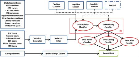
A simplified architecture of our system is shown in Figure 1. Unstructured notes are first processed with a collection of trigger lexicons. The first type of trigger lexicon targets medical concepts, covering diabetes mentions, CAD mentions, CAD events, CAD tests, CAD symptoms, hyperlipidemia mentions, hypertension mentions, obesity mentions, smoker mentions, and 18 different classes of medications. The second type of trigger lexicon targets measurements, containing base names for measurements within the note whose value is the result of the measurement. This lexicon type includes A1c, glucose, total cholesterol, LDL, blood pressure, and BMI (the waist circumference measurement is in the guidelines but not our system due to the lack of data). Each measurement base is paired with its value as determined by a regular expression (e.g., A1c is a real value with optionally one digit after the decimal) and a min/max range (e.g., in the range (0,100) for A1c, though the extreme values are admittedly unlikely). Measurements can therefore be considered a relation between base and value. At test time, the measurements are further filtered to only include those above the specified threshold. The third type of lexicon includes immediate family relations (e.g., mother, brother) for family history detection, which is a rule-based system and therefore separated from the other triggers. Table 3 reports the number of terms in each lexicon.

Figure 1.

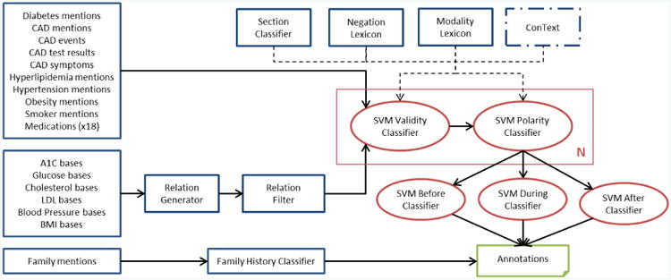
System architecture. Blue borders indicate rule-based modules while red borders indicate machine learning-based modules. N indicates there are different classification models for each annotation type. The primary exception to this architecture is the Smoker mention approach.

Table 3.

Number of terms in each annotation lexicon.

Annotation	Base Terms	Pre-Modifiers	Post-Modifiers
Diabetes Mention	20	30	44
A1C	37	-	-
Glucose	12	-	-
CAD Mention	7	2	-
CAD Event	31	-	-
CAD Test Result	18	-	-
CAD Symptom	6	-	-
Hyperlipidemia Mention	19	3	-
Cholesterol	4	-	-
LDL	3	-	-
Hypertension Mention	12	3	-
Blood Pressure	10	-	-
Obese Mention	4	6	-
BMI	1	-	-
Smoker Mention	25	13	13
Medication	565	-	-

After trigger extraction, the candidate risk factors go through a series of support vector machine (SVM) [26] classifiers that (1) filter out invalid triggers, (2) filter out negated triggers, and (3) classify time with three separate binary classifiers. Different SVM models are used by the validity and polarity classifiers for each annotation type, while each of the three time classifiers uses one model for all annotation types. The features used in all the classifiers are described below. The output of the three time classifiers is then subject to a set of constraints and exceptions:

1. Diabetes, CAD, hyperlipidemia, hypertension, and obesity mentions are assumed to be [before DCT, during DCT, after DCT] (i.e., all times). They therefore do not go through time classifiers.

2. A1c, glucose, CAD events, CAD test result, CAD symptoms, cholesterol, LDL, blood pressure, and BMI are assumed to have exactly one time. Therefore, the highest confidence positive result of the three time classifiers is used to determine their time.

3. Medications are the only annotation type with an unconstrained time. All three time classifiers are run and the corresponding times are assigned if the positive confidence is greater than the negative.

4. Smoker mentions are not run through either the time classifiers or a polarity classifier. Instead, a 5-way classifier is used to assign the smoking status, as explained below.

5. Glucose requires two measurements over 126. Therefore, if only one glucose measurement is present in a note, it is removed prior to time classification.

The features used in our classifiers are shown in Table 4. The first set of features is used in every classifier. The second set is used only in the measurement validity and polarity classifiers. The third set is used only in the three time classifiers. For the most part, the features used were quite simple, and chosen entirely based on our intuition for the ways in which validity, polarity, and temporality were expressed in the corpus. To illustrate these features, consider the following two examples, where the relevant risk factor spans are in bold:

1. He has a history of diabetes and sleep apnea.

2. His hemoglobin A1c was 7.4 % a month ago.

Table 4. Features used in ML classifiers.

All classifiers
F1 Indexed uncased previous words
F2 Indexed uncased next words
F3 Generic words within 5 tokens
F4 Has family term within 5 tokens
F5 Negation word in previous 10 tokens
F6 Modality word in previous 10 tokens
F7 ConText negation value
F8 ConText history value
F9 ConText hypothetical value
F10 ConText experiencer value
F11 Section name
Measurement classifiers only	Time classifiers only
F12 Words between base and value	F18 Annotation type
F13 Word shapes between base and value	F19 Medication type
F14 Value shape
F15 Base and value on same line
F16 Number of tokens between base and value
F17 Target word in previous 5 tokens

The first set of features provides simple external context. Since a different model is used for each risk factor, the internal information (e.g., whether the risk factor is spelled diabetes or DM) was largely irrelevant. These features are:

• F₁ and F₂ are simple contextual features to represent the caseless words before and after, respectively, the risk factor. For (1), F₁ would be {1:of, 2:history, 3:a, 4:has, 5:he}, while F₂ would be {1:and, 2:sleep, 3:apnea}.

• F₃ is a bag-of-words feature for a 5-word context around the risk factor where case is removed from words and numbers are replaced with 0. For (1), F₃ would be {a, apnea, has, he, history, of, sleep}.

• F₄ is a binary feature indicating whether a family word is in a 5-token context. This helps identify cases where the risk factor is associated with a family member and not the patient. The family member lexicon has 28 terms, including more than just the immediate family, as well as plural words (e.g., grandparents, aunts). Neither (1) nor (2) have such a word.

• F₅ and F₆ use negation and modality lexicons, respectively, to identify words in the 10 previous tokens that might indicate negation, modality, or temporality. These lexicons were first proposed in Kilicoglu & Bergler [27]. The negation lexicon includes words like hasn't, exclude, and prevent. The modality lexicon includes words like attempt, potentially, and unknown.

• F₇ to F₁₀ use the ConText algorithm [10] to provide contextual clues about negation (negated vs. affirmed), history (historical vs. recent), hypotheticality (not particular vs. recent), and experiencer (other vs. patient).

• F₁₁ provides the name of the section using a simple heuristic. The closest previous line ending in acolon and containing less than 10 tokens is considered the section header.

The second set of features provides internal context for measurements. Since the measurement candidate extraction simply looks for compatible base and value pairs within a reasonable distance, often the base and value do not correspond to each other (e.g., multiple measurements in the same sentence). The measurement features therefore are designed to indicate the relatedness between the base and value:

• F₁₂ is a bag-of-words feature between the base and value. For (2), F₁₂ would be {was}.

• F₁₃ is a bag-of-wordshapes feature between the base and value, where a wordshape is a case representation where all upper case letters are replaced with A, all lower case letters are replaced with a, and all numbers are replaced with 0. For (2), F₁₃ would be {aaa}.

• F₁₄ is the shape of the value, which helps capture legal types of values. For (2), F₁₄ would be {0.0}.

• F₁₅ is a binary feature that indicates whether the base and value are on the same line. In most cases this is true for gold measurements, but occasionally the measurements are located in multi-line tables which requires expanding the context beyond the line.

• F₁₆ indicates the token distance between the base and value. For (2), F₁₆ would be 1.0.

• F₁₇ is a binary feature that indicates if a “target” word is in the previous 5 tokens. Commonly, the notes express a desired measurement instead of an actual measurement (e.g., “target A1c value is 7.5” or “shooting for A1c of 8.0)”. This feature uses a lexicon of 17 target synonyms to help capture these cases.

The third set of features only applies to the time classifiers. Since all risk factors are classified with the same 3 time models, the two features in this set distinguish between the type of risk factor under the assumption that different risk factors have different temporal properties:

• F₁₈ indicates the type of annotation (e.g., A1C, Blood_pressure, Medication).

• F₁₉ indicates the type of medication (e.g., fibrate, diuretic, aspirin), and ignores non-medications.

Since smoking status is not binary, the heuristic of a single positive mention indicating the entire note is positive does not apply. Instead, the smoking status SVM is a document-level classifier. It uses the same set of base features, but the individual features for every valid smoking mention in the note is aggregated into a single feature. For example, with feature F₁₁, instead of returning a single section name for the smoker mention, F₁₁ returns the section names for all the smoker mentions in the note.

Finally, the family history of CAD module is a simple rule-based system that combines a lexicon of immediate family names with the output annotations from the previously described classifiers. The lexicon consists of 6 immediate family relations (father, mother, brother, sister, son, daughter). Within the immediate context (10 tokens) of one of these terms, a valid, non-negated CAD-related annotation (CAD mention or CAD event) must be present with an age below the specified threshold (55 for male, 65 for female) for the family history attribute to be considered Present. Otherwise the family history attribute is considered NotPresent. Additionally, if a synonym of the phrase “family history” appears with a CAD-related annotation, the presence of a family history of CAD is assumed regardless of age (since it is un-specified). In all cases, no syntactic processing is used, simply the presence of terms matching those described above within the local context is assumed to be an indication of a family history of CAD.

6 Results

The official results for our first two runs are shown in Table 5, along with the official aggregate results and other top submissions. Our third run performed worse on every measure and is omitted. Run #1 has the best recall of the two runs, while Run #2 has the best precision and F₁-measure. Run #1 is the system as described in the Risk Factor Identification section. Run #2 is essentially the same, but with two filtering steps to improve precision. First, all glucose results are removed since the vast majority of the glucose measurements in the gold data are not annotated as a risk factor, which results in models that predict large amounts of false positives. Second, a set of 52 low-precision triggers is filtered out (e.g., chest for CAD symptom, substance for smoker mention). These two filtering steps raise precision considerably (0.8702 to 0.8951) without a large drop in recall (0.9694 to 0.9625), thus raising the overall F₁-measure (0.9171 to 0.9276).

Table 5.

Official submission results, sorted by micro-F₁, including our two submissions, aggregate results, and other top submissions.

System	Micro			Macro
	P	R	F1	P	R	F1
NLM Run #2 (1st)	0.8951	0.9625	0.9276	0.8965	0.9611	0.9277
Harbin (2nd)	0.9106	0.9436	0.9268	0.9119	0.9399	0.9257
Kaiser Permanente (3rd)	0.8972	0.9409	0.9185	0.8998	0.9429	0.9209
Linguamatics (4th)	0.8975	0.9375	0.9171	0.8989	0.9361	0.9171
NLM Run #1	0.8702	0.9694	0.9171	0.8694	0.9682	0.9162
Nottingham (5th)	0.8847	0.9488	0.9156	0.8885	0.9411	0.9141
Median	0.852	0.908	0.872	0.849	0.904	0.870
Mean	0.808	0.835	0.815	0.800	0.834	0.812
Min	0.455	0.203	0.305	0.455	0.258	0.365

The per-annotation type results for Run #2 are shown in Table 6. Compared to the overall F₁-measure for the run (micro 0.9276, macro 0.9277), many of the risk factors perform much better or worse. Every mention annotation except CAD outperforms the overall F₁, while every measurement annotation under-performs the overall F₁. For all but 6 of the annotations, recall outperformed precision. Additionally, for the lower performing risk factors, if one ignores the time attribute, their performances are significantly improved. Most of the individual validity and polarity classifiers achieve a classification accuracy of over 95%. Much of the loss, therefore, comes from time classification. This is why many of the chronic diseases, which are almost always [before DCT, during DCT, after DCT], have high overall performance, while many of the measurements have lower overall performance.

Table 6.

Results by risk factor for Run #2. Notes: (1) Glucose was omitted from this run. (2) Smoking status is a 5-way classification, hence precision and recall should be identical and equal to the accuracy. However, some documents are inadvertently missing a smoking status, so only the recall is equal to the accuracy on the sub-set of documents with a smoking status. (3) There are no examples of Amylin in either the training or test data, while only the training data contains examples of anti diabetes medications.

Type	Risk Factor	P	R	F1
Diabetes	Mention	0.9568	0.9972	0.9766
	A1C	0.8235	0.8537	0.8383
	Glucose	-	-	-
	ALL	0.9473	0.9593	0.9533
CAD	Mention	0.8705	0.9767	0.9205
	Event	0.6719	0.9281	0.7795
	Test Result	0.4425	0.8475	0.5814
	Symptom	0.6170	0.4143	0.4957
	ALL	0.7648	0.9082	0.8303
Hyperlipidemia	Mention	0.9419	0.9578	0.9498
	Cholesterol	0.6000	0.5455	0.5714
	LDL	0.7333	0.7586	0.7458
	ALL	0.9292	0.9441	0.9366
Hypertension	Mention	0.9581	1.0000	0.9786
	Blood Pressure	0.7627	0.9231	0.8353
	ALL	0.9247	0.9884	0.9555
Obesity	Mention	0.9325	0.9592	0.9457
	BMI	0.7692	0.5882	0.6667
	ALL	0.9245	0.9351	0.9298
Family History	Present	0.8000	0.6316	0.7059
	Accuracy		0.9805
Smoking	Status		0.8555
Medication	ACE Inhibitor	0.8754	0.9707	0.9206
	Amylin	-	-	-
	Anti Diabetes	-	-	-
	ARB	0.8972	0.9948	0.9435
	Aspirin	0.9427	0.9887	0.9651
	Beta Blocker	0.9019	0.9904	0.9441
	Calcium Channel Blocker	0.9031	0.9688	0.9348
	Diuretic	0.7955	0.9646	0.9719
	DPP4 Inhibitor	1.0000	0.8333	0.9091
	Ezetimibe	0.7805	0.8889	0.8312
	Fibrate	0.9195	0.8889	0.9040
	Insulin	0.8588	0.9544	0.9041
	Metformin	0.8561	0.9946	0.9202
	Niacin	0.6250	1.0000	0.7692
	Nitrate	0.7723	1.0000	0.7692
	Statin	0.9301	0.9767	0.9528
	Sulfonylurea	0.9135	0.9896	0.9500
	Thiazolidinedione	0.8406	0.9508	0.8923
	Thienopyridine	0.9213	0.9894	0.9542
	ALL	0.8890	0.9766	0.9307

7 Discussion

7.1 Error Analysis

As the results in the previous section show, our system is heavily skewed toward recall. To some extent, this is a natural result of our system's design: the lexicons are high-recall by design, and most of the validity and polarity classifiers are trained on data that is heavily skewed positive. While the gold test data contains 10,974 annotations, our system output 11,801 annotations (almost 8% more). This evaluation is complicated, however, by the way times were evaluated. No partial credit is given for an incorrect time, and risk factors that occur before, during, and after the hospital visit receive three times the amount of credit as a risk factor with only one time. Biasing toward recall can thus help here: guessing [before DCT, during DCT] for a risk factor that is only [during DCT] results in an F₁-measure of 66.7, while guessing just [before DCT] results in an F₁-measure of 0.0. Upon examination of the precision errors made by the system, the majority were indeed due to an excessive emphasis on recall. This includes medications in the allergy section (i.e., should have been negated, but their presence in a list structure meant there was no local context cues) as well as those with a super-set of the valid times (e.g., marking discontinued medications as after DCT in addition to before DCT and during DCT). There were some examples, though, of mentions missed by the original annotators and picked up by our system, possibly including following examples:

1. A 75-year-old diabetic whose glycemic control is good.

2. His CRF include HTN, elevated cholesterol, smoking, male gender.

3. 2/02: A1c 6.50.

4. Test Description	Result	Abnormal Flag	Ref. Range	Ref. Units
   … (table) …
   Cholesterol	245			mg/dl

The first example is a diabetes mention that was missed by the annotators, likely because it is the adjective form instead of the noun (it was observed at least once in the training data, however, and was therefore in our lexicon). In the second example, “elevated cholesterol” is generally considered to be a hyperlipidemia mention in the training data, as well as much of the test data. In the third example, while 6.5 is not strictly “over 6.5”, many times in the training data an A1c of 6.5 was marked as a high A1c value. In the fourth example, the total cholesterol's value is located within a tabular structure (tables, in general, were not only difficult for the automatic system, but they also were time-consuming to annotate due to the large number of quantitative values).

These examples demonstrate the difficulty of attempting to replicate the implicit annotation standard used by the original annotators. During our annotation process, when a question arose as to the legitimacy of a certain annotation, we generally consulted the training data. If around half the times in the training data (or more) a phrase was annotated a particular way, our annotators were instructed to do that as well. When a question arose where no example in the training data existed to guide our decisions, we relied on the clinical expertise of the annotators to determine if the given risk factor applied to the patient. In general, we erred on the side of recall. In practice, this again resulted in ML classifiers with unbalanced data, creating clear errors in our output. An example is this case where the abbreviation NG is mistaken for a nitrate, since it was used that way once in the training data and thus appeared in our lexicon:

• 5. NG tube lavage showed 200 cc of pink tinged fluid, cleared after 50 cc.

Other low-precision examples include “chest” in the CAD mention lexicon and “cholesterol” in the hyperlipi-demia lexicon. While these examples were used at least once as positive mentions in the original data, it was felt that they had sufficiently low precision that we removed these and other mention candidates (a total of 52 different lexicon items) for Run #2, which outperformed Run #1 in both precision and F₁ at the cost of a small drop in recall. Ideally, the classifiers would have filtered these errors out to maintain the superior recall, but it is likely there was not sufficient data for the classifiers to properly handle these fairly rare terms. Integration of methods for abbreviation disambiguation [28] and concept normalization [29] could potentially handle such cases without any additional data directly related to this task, as each of those methods indirectly incorporates additional data into their models.

The CAD event, test result, and symptom risk factors are some of the most difficult to annotate (Table 2) as well as detect automatically (Table 6). While the original annotations generally had predictable spans, and normalization typically involved adding or removing a few words, the three non-mention CAD risk factors often had entirely unpredictable spans in the original annotations. For example, the following typify the provided annotations:

• Event: “s/p ant SEMI + stent LAD”, “PTCA w/ Angioplasty to LAD”

• Test Result: “Stress (3/88): rev. anterolateral ischemia”, “normal ECG but a small anteroseptal zone of ischemia”

• Symptom: “occasional and very transient episodes of angina”, “Since 11/19/2096 he has had complaints of increasing dyspnea on exertion and chest pain”

These were shortened in our lexicon to one-word terms such as “infarction” and “stent” for event, “ecg” and “catheterization” for test result, and “angina” and “cp” (chest pain) for symptom. However, our main reason for normalization was to learn consistent lexical context, but the loose descriptions seen above meant that many of the contexts in the test data were never seen in the training data. Due to the diversity of phrasing, we attempted to find the most minimal set of lexicon terms to cover all the cases in the training data. Thus, we chose “chest” instead of “chest pain” for symptoms to cover cases such as “a dull and mid scapular discomfort that radiated to his upper chest”. However, it was found that “chest” was too imprecise and was removed for Run #2 without adding “chest pain” to the lexicon. This missing term alone probably accounts for a significant loss of recall for CAD symptoms. Instead of mention-level classification, these risk factors may perhaps be better suited for sentence classification, where n-gram features can overcome the sparsity in phrases.

A surprising result was the poor performance on BMI, as our method performed quite well on BMI with the training data. There were not very many BMI instances in the data, however: Run #2 had 10 true positives, 3 false positives, and 7 false negatives. The false positives are indeed system errors: one marked a BMI of 30 when the standard requires over 30 (though for other measurements in the training data, values at the threshold were sometimes marked as positive), and twice a [during DCT] was marked as a [before DCT], which also resulted in two false negatives. Four of the false negatives (recall errors) could easily be argued to be annotation mistakes: twice a BMI was marked as [before DCT, during DCT, after DCT] when the system classified [during DCT] despite the annotation convention generally favoring marking only a single time for a measurement. The final false negative was the result of the note providing a height and weight, implicitly allowing for a BMI calculation, but the actual BMI was not in the note (this type of BMI annotation never came up in the training data).

Several of the errors made by our system were the result of our additional annotations. Ultimately, given that the original annotations and the NLM annotations were created by two different sets of annotators, and without a highly detailed guideline to ensure consistency, it would be impossible to expect the two sets of annotations to line up perfectly. A prime example of this is the glucose annotation, which was annotated in only 24 documents in the original training data, but was labeled by our annotators hundreds of times. Even when applying the “two times” filter, there were still far more glucose measurements using our annotations. As a result, we removed them from Run #2, resulting in a large precision gain for a small drop in recall.

7.2 System Design

A notable aspect about our system is its lack of reliance on many third-party tools to provide higher-level linguistic information, such as syntax and semantics. This has inherent advantages on its own, since many tools (e.g., a part-of-speech tagger) demonstrate significant performance variation on different texts. However, we make no claim that such information would not have improved our performance further on this task. It is quite likely our performance would have been even higher if we had incorporated parts-of-speech, syntactic dependencies, named entities, ontological knowledge, and more. This type of information was certainly beneficial to other participants in the 2014 i2b2 task. Actually, very little work was done at all in feature engineering. The set of features in Table 4 were chosen completely based on our sense of the important lexical information that could be captured. Removing some of the features might easily help the score, and there are certainly other lexical features worth adding. No experiments were attempted to adjust this initial feature set, largely due to the time-consuming nature of feature engineering. Such experiments, as well as adding syntactic and semantic features, would almost certainly have increased system performance. Due to the significant number of such features in the literature, however, we leave such improvements to future work. Despite this, it should be noted that even without the lack of risk factor customization, the performance across the mention-type annotations is quite good, all of which have an F₁-measure of at least 0.92. Our method, therefore, would likely generalize well to other diseases with similar data, though certainly disease-specific processing would be ideal.

Given the limited amount of time available for system development in the 2014 i2b2 task, we simply chose to devote our resources instead to creating more fine-grained annotations. Importantly, this is analogous to a very common real-world problem when developing NLP systems: given limited resources (time, funding, etc.), are those resources better spent (a) developing more advanced systems, or (b) creating higher quality data? While there is no one absolutely correct answer, and while we make no claim as to the generalizability of our results beyond the 2014 i2b2 task, these results do provide an interesting case study to help explore this important question.

One way to evaluate the effect of the fine-grained annotations is simply to examine the system rankings in Table 5. Instead, we would prefer some quantitative measure of the value of these fine-grained annotations independent of the system itself. That is, if we had two nearly identical systems, one with access to the fine-grained annotations and one without, how would these systems compare? To do this, we utilize the same basic information extraction approach: identical lexicons, architecture, ML features. The main factors to remove are the NLM annotations (both positive and negative) and the normalized concept boundaries. We thus consider four different systems, with increasing reliance on the NLM annotations:

• nonorm: Uses only the original, uncorrected annotations provided by the organizers. Since this leaves only positive mention-level annotations, we use a heuristic to create negative annotations: any lexicon match in a negative document is considered a negative annotation.

• norm: Same as nonorm, but the boundaries in the original annotations are normalized to be consistent with the lexicon.

• goldneg: Same as Norm, but instead of the heuristically annotated negative concepts, the NLM-annotated negative gold concepts are used.

• run2: The official NLM Run #2. Same as goldneg, except all NLM-annotated gold concepts are used (i.e., includes additional positive annotations).

The results on these four experiments are shown in Table 7. The nonorm method (i.e., the system without any changes to the original annotations) would only have achieved an F₁-measure of 0.9021, a large drop compared to the submitted F₁ of 0.9276. This would have only been enough for 7th place in the task, which is still above the median but not at all close to the top participants. The Norm method, which didn't add any additional annotations but changed the boundaries of the original annotations to be more consistent with the lexicon, shows a slight improvement (from 0.9021 to 0.9043). This gain is likely due to the fact that the risk factors' context in the training data is better captured with the more consistent span boundaries. Additionally, there were several dozen incorrect annotations that were removed from the original data, which is reflected in this score as well.

Table 7.

Post-hoc experiments with varying degrees of reliance on the NLM annotations. Place is the theoretical ranking (micro F₁) had the given system been submitted as an official result.

System	Micro			Macro			Place
	P	R	F1	P	R	F1
nonorm	0.8470	0.9648	0.9021	0.8456	0.9629	0.9005	7th
norm	0.8506	0.9652	0.9043	0.8484	0.9630	0.9021	7th
goldneg	0.9030	0.9579	0.9296	0.9041	0.9560	0.9294	1st
run2	0.8951	0.9625	0.9276	0.8965	0.9611	0.9277	-

The goldneg results show the very large improvement made by adding the manually-labeled negative annotations (from 0.9043 to 0.9296). Interestingly, this F₁-measure is higher than that from run2. This means that while adding the gold negatives provided a large boost in performance, adding gold positives actually hurt slightly. The most likely explanation for this is the lack of annotation alignment between the original annotators and the NLM annotators. While the benefit of negative annotations far outweighed the cost of mis-aligned negative annotations, there was insufficient benefit in the additional positive annotations to overcome the disagreement between the two annotator groups. We can speculate this would not have been the case if (a) the same set of annotators labeled both data sets, or (b) extremely detailed annotation guidelines were provided to increase the inter-group agreement.

These observations lead us to several points for potentially improving the system used in Run #2. First, either the NLM-annotated positive concepts should be removed, or a deeper investigation should be performed to determine the key points of inter-group disagreement. Second, further experiments with the lexical ML features should be performed to determine if any of the features in Table 4 actually degrade performance, or if any other lexical features improve performance. Third, further experiments with syntactic, semantic, and discourse-level features should be performed to assess what additional value they may provide. The features utilized by other top-performing systems in the 2014 i2b2 task are a useful starting point for such features.

8 Conclusion

This article has described our submission to the 2014 i2b2 task, which was a fairly simple supervised information extraction method based on lexicons and mention-level classification. Our key contribution to the task was a large set of mention-level annotations for the various heart disease risk factors. We have explored the impact of fine-grained annotations, both manually and heuristically labeled, to assess the value of this data. Despite being a relatively simple system that employs only lexical features, our submission achieved the high-est scores (micro- and macro-F₁, and micro- and macro-recall) out of the 20 participants. The official results of this task, as well as the post-hoc experiments we performed, demonstrate the importance of high-quality, fine-grained natural language annotations.

1. Supervised information extraction to identify risk factors for heart disease in EHRs.

2. Approach achieved the highest overall F₁-measure on the 2014 i2b2 challenge.

3. Finer-grained annotations are used over those provided by the organizers.

4. Approach relies on lexical features that are mediocre with the original annotations.

5. Demonstrates a simple approach with better data can outperform more advanced NLP.

References

- 1.Stubbs Amber, Kotfila Christopher, Xu Hua, Uzuner Özlem. Practical applications for NLP in Clinical Research: the 2014 i2b2/UTHealth shared tasks. J Biomed Inform. 2015 doi: 10.1016/j.jbi.2015.10.007. [DOI] [PMC free article] [PubMed] [Google Scholar]
- 2.Uzuner Özlem, South Brett, Shen Shuying, DuVall Scott L. 2010 i2b2/VA challenge on concepts, assertions, and relations in clinical text. J Am Med Inform Assoc. 2011;18:552–556. doi: 10.1136/amiajnl-2011-000203. [DOI] [PMC free article] [PubMed] [Google Scholar]
- 3.Uzuner Özlem, Bodnari Andreea, Shen Shuying, Forbush Tyler, Pestian John, South Brett. Evaluating the state of the art in coreference resolution for electronic medical records. J Am Med Inform Assoc. 2011;18:552–556. doi: 10.1136/amiajnl-2011-000784. [DOI] [PMC free article] [PubMed] [Google Scholar]
- 4.Sun Weiyi, Rumshisky Anna, Uzuner Ozlem. Evaluating Temporal Relations in Clinical Text: 2012 i2b2 Challenge Overview. J Am Med Inform Assoc. 2013;20(5):806–813. doi: 10.1136/amiajnl-2013-001628. [DOI] [PMC free article] [PubMed] [Google Scholar]
- 5.Demner-Fushman Dina, Chapman Wendy W, McDonald Clement J. What can Natural Language Processing do for Clinical Decision Support? J Biomed Inform. 2009;42(5):760–772. doi: 10.1016/j.jbi.2009.08.007. [DOI] [PMC free article] [PubMed] [Google Scholar]
- 6.Aronson AR, Lang FM. An overview of MetaMap: historical perspective and recent advances. J Am Med Inform Assoc. 2010;17:229–236. doi: 10.1136/jamia.2009.002733. [DOI] [PMC free article] [PubMed] [Google Scholar]
- 7.Friedman Carol. A broad-coverage natural language processing system. Proceedings of the AMIA Annual Symposium. 2000:270–274. [PMC free article] [PubMed] [Google Scholar]
- 8.Savova Guergana K, Masanz James J, Ogren Philip V, Zheng Jiaping, Sohn Sunghwan, Kipper-Schuler Karin C, Chute Christopher G. Mayo clinical Text Analysis and Knowledge Extraction System (cTAKES): architecture, component evaluation and applications. J Am Med Inform Assoc. 2010;17:507–513. doi: 10.1136/jamia.2009.001560. [DOI] [PMC free article] [PubMed] [Google Scholar]
- 9.Chapman Wendy W, Bridewell Will, Hanbury Paul, Cooper Gregory F, Buchanan Bruce G. A Simple Algorithm for Identifying Negated Findings and Diseases in Discharge Summaries. J Biomed Inform. 2001 Oct;34(5):301–310. doi: 10.1006/jbin.2001.1029. [DOI] [PubMed] [Google Scholar]
- 10.Harkema Henk, Dowling John N, Thornblade Tyler, Chapman Wendy W. ConText: An algorithm for determining negation, experiencer, and temporal status from clinical reports. J Biomed Inform. 2009;42(5):839–851. doi: 10.1016/j.jbi.2009.05.002. [DOI] [PMC free article] [PubMed] [Google Scholar]
- 11.Pradhan S, Elhadad N, South BR, Martinez D, Christensen L, Vogel A, Suominen H, Chapman WW, Savova G. Evaluating the state of the art in disorder recognition and normalization of the clinical narrative. J Am Med Inform Assoc. 2015;22(1):143–154. doi: 10.1136/amiajnl-2013-002544. [DOI] [PMC free article] [PubMed] [Google Scholar]
- 12.Uzuner Özlem, Luo Yuan, Szolovits Peter. Evaluating the State-of-the-Art in Automatic De-Identification. J Am Med Inform Assoc. 2007;14(5):550–563. doi: 10.1197/jamia.M2444. [DOI] [PMC free article] [PubMed] [Google Scholar]
- 13.Uzuner Özlem, Goldstein Ira, Luo Yuan, Kohane Isaac. Identifying Patient Smoking Status from Medical Discharge Records. J Am Med Inform Assoc. 2008;15(1):15–24. doi: 10.1197/jamia.M2408. [DOI] [PMC free article] [PubMed] [Google Scholar]
- 14.Uzuner Özlem. Recognizing Obesity and Co-morbidities in Sparse Data. J Am Med Inform Assoc. 2009;16(4):561–570. doi: 10.1197/jamia.M3115. [DOI] [PMC free article] [PubMed] [Google Scholar]
- 15.Uzuner Özlem, Solti Imre, Cadag Eithon. Extracting Medication Information from Clinical Text. J Am Med Inform Assoc. 2010;17:514–518. doi: 10.1136/jamia.2010.003947. [DOI] [PMC free article] [PubMed] [Google Scholar]
- 16.Pestian John P, Matykiewicz Pawel, Linn-Gust Michelle, South B, Uzuner Ozlem, Wiebe Jan, Cohen B, Hurdle John, Brew Christopher. Sentiment Analysis of Suicide Notes: A Shared Task. Biomedical Informatics Insights. 2012;5(Suppl. 1) doi: 10.4137/BII.S9042. [DOI] [PMC free article] [PubMed] [Google Scholar]
- 17.Cimino James J, Bright Tiffani J, Li Jianhua. Medication Reconciliation Using Natural Language Processing and Controlled Terminologies. Studies in Health Technology and Informatics (MEDINFO) 2007:679–683. [PubMed] [Google Scholar]
- 18.Gold Sigfried, Elhadad Noémie, Zhu Xinxin, Cimino James J, Hripcsak George. Extracting structured medication event information from discharge summaries. Proceedings of the AMIA Annual Symposium. 2008:237–241. [PMC free article] [PubMed] [Google Scholar]
- 19.Goryachev Sergey, Kim Hyeoneui, Zeng-Treitler Qing. Identification and Extraction of Family History Information from Clinical Reports. Proceedings of the AMIA Annual Symposium. 2008:247–251. [PMC free article] [PubMed] [Google Scholar]
- 20.Lewis Neal, Gruhl Daniel, Yang Hui. Extracting Family History Diagnoses from Clinical Texts. Proceedings of the 3rd International Conference on Bioinformatics and Computational Biology (BICoB) 2011:128–133. [Google Scholar]
- 21.Friedlin Jeff, McDonald Clement J. Using A Natural Language Processing System to Extract and Code Family History Data from Admission Reports. Proceedings of the AMIA Annual Symposium. 2006:925. [PMC free article] [PubMed] [Google Scholar]
- 22.Zhou Li, Melton Genevieve B, Parsons Simon, Hripcsak George. A temporal constraint structure for extracting temporal information from clinical narrative. J Biomed Inform. 2006;39(4):424–439. doi: 10.1016/j.jbi.2005.07.002. [DOI] [PubMed] [Google Scholar]
- 23.Bramset Philip, Deshpande Pawan, Lee Yoong Keok, Barzilay Regina. Finding Temporal Order in Discharge Summaries. Proceedings of the AMIA Annual Symposium. 2006:81–85. [PMC free article] [PubMed] [Google Scholar]
- 24.D'Souza Jennifer, Ng Vincent. Knowledge-rich temporal relation identification and classification in clinical notes. Database. 2014:1–20. doi: 10.1093/database/bau109. [DOI] [PMC free article] [PubMed] [Google Scholar]
- 25.Stubbs Amber, Uzuner Özlem. Annotating Risk Factors for Heart Disease in Clinical Narratives for Diabetic Patients. J Biomed Inform. 2015 doi: 10.1016/j.jbi.2015.05.009. [DOI] [PMC free article] [PubMed] [Google Scholar]
- 26.Fan RE, Chang KW, Hsieh CJ, Wang XR, Lin CJ. LIBLINEAR: A Library for Large Linear Classification. Journal of Machine Learning Research. 2008;9:1871–1874. [Google Scholar]
- 27.Kilicoglu Halil, Bergler Sabine. Syntactic Dependency Based Heuristics for Biological Event Extraction. Proceedings of the BioNLP 2009 Workshop Companion Volume for Shared Task. 2009:119–127. [Google Scholar]
- 28.Wu Yonghui, Denny Joshua C, Rosenbloom S Trent, Miller Randolph A, Giuse Dario A, Xu Hua. A comparative study on current clinical natural language processing systems on handling abbreviations in discharge summaries. Proceedings of the AMIA Annual Symposium. 2012:997–1003. [PMC free article] [PubMed] [Google Scholar]
- 29.Leaman Robert, Doğan Rezarta Islamaj, Lu Zhiyong. DNorm: disease name normalization with pairwise learning to rank. Bioinformatics. 2013;29(22):2909–2917. doi: 10.1093/bioinformatics/btt474. [DOI] [PMC free article] [PubMed] [Google Scholar]