The effects of sampling strategy on the quality of reconstruction of viral population dynamics using Bayesian skyline family coalescent methods: A simulation study

Abstract

The ongoing large-scale increase in the total amount of genetic data for viruses and other pathogens has led to a situation in which it is often not possible to include every available sequence in a phylogenetic analysis and expect the procedure to complete in reasonable computational time. This raises questions about how a set of sequences should be selected for analysis, particularly if the data are used to infer more than just the phylogenetic tree itself. The design of sampling strategies for molecular epidemiology has been a neglected field of research. This article describes a large-scale simulation exercise that was undertaken to select an appropriate strategy when using the GMRF skygrid, one of the Bayesian skyline family of coalescent methods, in order to reconstruct past population dynamics. The simulated scenarios were intended to represent sampling for the population of an endemic virus across multiple geographical locations. Large phylogenies were simulated under a coalescent or structured coalescent model and sequences simulated from these trees; the resulting datasets were then downsampled for analyses according to a variety of schemes. Variation in results between different replicates of the same scheme was not insignificant, and as a result, we recommend that where possible analyses are repeated with different datasets in order to establish that elements of a reconstruction are not simply the result of the particular set of samples selected. We show that an individual stochastic choice of sequences can introduce spurious behaviour in the median line of the skygrid plot and that even marginal likelihood estimation can suggest complicated dynamics that were not in fact present. We recommend that the median line should not be used to infer historical events on its own. Sampling sequences with uniform probability with respect to both time and spatial location (deme) never performed worse than sampling with probability proportional to the effective population size at that time and in that location and frequently was superior. As a result, we recommend this approach in the design of future studies. We also confirm that the inclusion of many recent sequences from a single geographical location in an analysis tends to result in a spurious bottleneck effect in the reconstruction and caution against interpreting this as genuine.

1. Introduction

The quantity of available genetic data on viruses and other pathogens is already very large and will only grow in future. The days when, in performing a phylogenetic analysis, it might be appropriate to use every sequence available simply as the result of scarcity of data are long gone for some species and cannot last long for many others. This raises the important question of how, in future, a set of sequences should be selected for analysis. There are two concerns here. Firstly, only very basic or approximate phylogenetic methods can analyse thousands of sequences in reasonable computational time, and those which can are often limited to reconstructing just the phylogeny itself; more sophisticated methods that fit epidemiological or population-genetic models to sequence data usually use Markov chain Monte Carlo (MCMC) procedures and often converge very slowly indeed on large datasets. Subsampling may be a necessity. Improved algorithms may eventually expedite procedures, and there are measures that could be employed at present to improve speed, for example, by reconstructing the phylogeny with a fast method and then using MCMC to estimate coalescence times and model parameters. However, the second problem will remain: a dataset consisting of every known sequence for a particular species will not have been sampled using any rigorous methodology, and the biases implicit in analysing one, or in any procedure by which one might be downsampled, must be considered. This has long been an important consideration in epidemiological studies; however, in molecular epidemiology, it has lagged as a concern, probably because in the past, genetic data of any sort has been at a premium. This must now start to be remedied.

In this article, we perform a large-scale simulation exercise to determine the effect of different sampling schemes on the reconstruction of the temporal dynamics of viral populations. The focus is on the design of sampling strategies for the investigation of the demographics of a large pathogen population causing endemic disease in diverse locations, rather than of an individual epidemic. For this reconstruction, we used the GMRF Skygrid plot (Gill et al. 2013). This is the most recent iteration in the Bayesian skyline family of methods (Drummond et al. 2005; Minin, Bloomquist, and Suchard 2008), which use coalescent theory to infer past variation in $N_{\text{e}}\tau$, the product of the effective population size (EPS) N_e, and the time between generations τ. Usually, no specific generation time is assumed and instead just the product is estimated. For brevity, when this article refers to ‘EPS’ it actually refers to this product. Unlike simple, parametric models of EPS (common examples of which are constant size, exponential growth, or logistic growth), the members of the skyline family are non-parametric: the timeline is divided up into a finite number of intervals, and the EPS is assumed to be constant on each interval but can vary between them. Its value on each interval is estimated along with the phylogeny.

While coalescent-based methods were originally conceived with populations of organisms in mind, such that the EPS is product of the (effective) number of individuals and the time between births, in viral studies it has often been interpreted in an epidemiological sense, so that the population is of infected individuals and the generation time the serial interval. This has been shown to be mathematically inaccurate (Frost and Volz 2010; Volz 2012); coalescence rates under an epidemiological model are governed by both incidence and prevalence and cannot generally be used to infer prevalence alone. For this reason, we prefer to regard population size estimates as representing the effective genetic diversity of the virus at the host population level. Skyline inference also makes the assumption that lineages form a single, freely mixing population. For this reason, and also because the relationship between effective and census population sizes is rarely straightforward, the numerical values of estimates of the EPS do not literally refer to a number of individuals, and exact interpretation of them is generally not attempted. Instead, temporal trends are examined for evidence of changes in population dynamics over time.

The assumption of free mixing will always be violated in practice. Structured coalescent models, which subdivide the total population into freely mixing ‘demes’ and allow lineages to transfer between them, are well developed (Notohara 1990). However, current implementations of these in phylogenetics packages assume that the size of each deme is constant over time (Vaughan et al. 2014; De Maio et al. 2015). As historical changes in population size are of considerable epidemiological interest, the skyline family is often still used, despite the fact that a key model assumption is generally invalid. One aim of this study is to investigate the effects of this discrepancy.

The effects of sampling strategy on phylogenetic and phylodynamic inference are a neglected area of study, which has been identified as an important future problem (Frost et al. 2015). The small number of papers that have previously explored sampling effects on demographic reconstruction in a context specific to inference of pathogen ancestries (Stack et al. 2010; de Silva, Ferguson, and Fraser 2012; Karcher et al. 2015) reconstructed dynamics from simulations in which the free-mixing assumption was not violated. To our knowledge, no published simulation study on the effects of sampling schemes has explored the effect of population structure in an infectious disease context. However, there are examples from the literature of eukaryotic phylogenetics. The most important difference between a study of that sort and an analysis appropriate to a pathogen study is that in the former case, the time periods between collections of samples are regarded as negligible compared to the evolutionary timescale, and hence all tips of the tree are treated as contemporaneous. This makes any consideration of the temporal nature of the sampling scheme irrelevant. A notable finding of these studies (Chikhi et al. 2010; Heller, Chikhi, and Siegismund 2013) is that spurious population bottlenecks tended to be detected if the sampling scheme was such that samples from some demes were missing.

Two of the three earlier pathogen studies simulated phylogenies under a mathematical model of transmission (Stack et al. 2010; de Silva, Ferguson, and Fraser 2012) and subsequently reconstructed the dynamics under a coalescent model. Volz (2012) demonstrated how to simulate phylogenies under a coalescent process whose underlying dynamics were a potentially complex model of transmission. Nevertheless, we chose to simulate our trees under a coalescent process in a Wright–Fisher population whose EPS obeyed a given function directly, for three reasons. First, because this is the model under which the skyline-family models perform their reconstructions. Second, because in the Volz solution, prevalence through time is derived as a function of birth and movement rates, and it is not straightforward to pick an arbitrary function of interest to represent the ‘true’ dynamics. Finally, the primary focus of this exercise was to investigate the effect of sampling scheme on the investigation of the global dynamics of an endemic disease. Constructing an epidemiological model for the behaviour of an endemic virus on an international scale raises many questions that are beyond the scope of this article; we found it preferable to use an established model for the population dynamics of a collection of organisms. So, while the exact relationship between the reconstructed EPSs from a coalescent model and the dynamics of infection is complex (Frost and Volz 2010; Volz 2012), we assume that such a relationship can be quantified and deal only with the effective size of the viral population. The demographic functions here were thus not intended to follow any particular model of disease dynamics; we instead investigated the quality of the reconstruction for various scenarios of variation in population size.

The finding of Chikhi et al. (2010) and Heller, Chikhi, and Siegismund (2013) that sampling from some populations and not others can falsely suggest population declines in reconstructed dynamics is pertinent to virus research, as it is a quite common practice in molecular epidemiological studies to analyse a large number of sequences recently collected as part of a single study with a more sparsely sampled dataset from other locations and times for comparison. This means that some subpopulations will be highly oversampled, and one might expect to see a dip in EPS estimates at the point in time at which the newly determined sequences were acquired. This pattern can, indeed, be seen in recent studies of foot-and-mouth disease virus (Hall et al. 2013), influenza A virus (Lin et al. 2011), West Nile virus (Phillips et al. 2014), and peste des petits ruminants virus (Padhi and Ma 2014). It makes intuitive sense that the population structure might confound the analysis in this case; under the assumption of random mixing, if a large number of lineages coalesce very rapidly before sampling, it would suggest a small total population size, but if the population was in fact structured (as will always be the case in reality) and these samples were all taken from the same place this would be misleading as they would coalesce only with those from the same deme. Nevertheless, this has not been explicitly demonstrated in a population analogous to a population of pathogens with non-contemporaneous temporal sampling.

2. Methods

2.1 Sequence simulation

We simulated ‘master’ datasets of 50,000 sequences under five demographic scenarios. The first two used a coalescent process occurring among an unstructured population of freely mixing haploid individuals. The EPS, $N_{\text{e}}\tau$, in each population varied with a deterministic function N(t). The overall phylogeny for 50,000 simulated isolates was constructed by, firstly, randomly placing 50,000 tree tips over a period of 10 time units; the units t were intended to represent years and will be referred to as such hereafter. The 10 years were divided into 10,000 intervals, and each sequence was assigned in turn to an interval with probability proportional to the function N evaluated at the midpoint of the interval. The exact sampling time was then selected by a draw from the uniform distribution with bounds confined to that interval. With all tips placed, coalescence was simulated until one lineage remained; for full details of the algorithm, see the Supplementary Material. The scenarios in which an unstructured population was used were as follows:

• Scenario 1: A population of constant size: N(t) = 10.

• Scenario 2: A population whose size underwent oscillations: $N(t)=10+7.5(\text{sin\hspace{0.17em}}\pi t)$.

The remaining three scenarios assumed a structured population, and trees were simulated under a structured coalescent. This involved a finite number of demes $D_1,\dots ,D_n$, and the EPS within each deme varied according to functions $N_1,\dots ,N_n$. A set of rates M_ij determined movement between demes, such that M_ij is twice the rate per year at which a lineage in deme D_i will move to deme D_j (Wakeley 2008). When simulating, tips were first assigned to a time interval as above, based on the total population size across all demes at the midpoint of the interval. They were then assigned to a deme with probability proportional to the EPS of that deme at that midpoint, and then to an exact time point within the interval as before.

Fig.1 depicts the population structure. The circles represent six demes $D_1,\dots ,D_6$: two small (D₁ and D₄), two medium (D₂ and D₅), and two large (D₃ and D₆). The exact relative sizes of these varied depending on the scenario. Arrows represent non-zero M_ij. Movement rates are symmetrical and invariant over time in all scenarios; thick arrows represent a rate of 0.05 per lineage (M_ij = 0.1) in the source population per year between the respective demes; thin arrows 0.025 (M_ij = 0.05). In this way, there is movement between each deme and four of the five others, two at a fast rate and two at a slow one. Let $s_i=i\mathrm{\hspace{0.17em}\hspace{0.17em}}(\text{mod}3)$. The demographic scenarios considered were as follows:

• Scenario 3: A structured population of constant size. $N_i(t)=10s_i/12$. Hence ${\displaystyle {\sum }_{i=1}^6{N}_i}(t)=10$ and the total EPS is the same as in Scenario 1.

• Scenario 4: A structured population in which the size of each deme experiences oscillations, and the oscillations are all in sync: $N_i(t)=s_i(10+7.5(\text{sin}\mathrm{\hspace{0.17em}\hspace{0.17em}}\pi t))/12$.

• Scenario 5: A structured population in which the size of each deme oscillates, but such that the EPS of each deme is in exact sync with two demes (of differing size to itself) and exactly out of sync with the remaining three:

  $$N_i(t)=\{\begin{array}{cc}{s}_i(10+7.5(\text{sin}\mathrm{\hspace{0.17em}\hspace{0.17em}}\pi t))/12& i\in \{1,3,5\}\\ s_i(10+7.5(\text{sin}\mathrm{\hspace{0.17em}\hspace{0.17em}}\pi (t+1)))/12& i\in \{2,4,6\}.\end{array}$$

Figure 1.

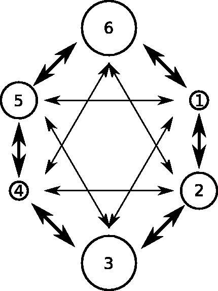
Depiction of the population structure used in structured coalescent simulations. Circles represent demes; two are small, two medium, and two large. Thick arrows represent fast rates of movement between demes (0.05 transitions per lineage per year) and thin arrows slower rates (0.025 per lineage per year).

Note that ${\displaystyle {\sum }_{i=1}^6{N}_i}(t)=10$; the total EPS is constant.

To convert the simulated ‘master’ phylogeny for each scenario to a set of sequences, the program $\pi$BUSS (Bielejec et al. 2014) was then used. This works by placing a random, ancestral sequence at the root of the tree and letting it evolve along the tree’s branches according to a stochastic model of sequence evolution. The sequence length and substitution process chosen was intended to roughly mimic the VP1 gene of foot-and-mouth disease virus; it had a length of 600 bp, and mutations occurred according to a strict molecular clock with a rate of $2.7\times {10}^{-3}$ substitutions per site per year. Mutations occurred according to the HKY substitution model (Hasegawa, Kishino, and Yano 1985) with a transition/transversion ratio of 2.718.

2.2 Subsampling for analysis

In every scenario, a variety of sampling schemes were used to select a subset of the master set for analysis. The 10-year sampling period was broken up into forty intervals. An interval was picked according to a temporal sampling scheme. In unstructured scenarios, a sequence was picked uniformly at random (without replacement) from the subset of the master set whose sequence dates were in this interval. For structured scenarios, where every sample in this subset was also annotated with a deme, a sequence was picked a spatial sampling scheme. This was repeated until the desired number of samples was achieved.

Temporal sampling schemes explored were:

• Uniform sampling: All intervals have equal probability.

• Proportional sampling: Intervals are chosen with probability proportional to the value of the demographic function describing the total EPS, evaluated at the midpoint of the interval.

• Reciprocal-proportional sampling: Intervals are chosen with probability proportional to the reciprocal of value of that demographic function.

Spatial sampling schemes explored were:

• Uniform sampling: All demes have equal probability.

• Proportional sampling: Demes are chosen with probability proportional to the EPS, relative to the EPSs of all other demes, of the deme at the midpoint of the interval.

• Reciprocal-proportional sampling: Demes are chosen with probability proportional to the reciprocal of the above.

In each scenario, all schemes under investigation were used to select a set of 300 samples, and this procedure was independently replicated fifty times. In addition, for Scenario 1, only we investigated the effect of sample size; this was done by taking five replicates of sample sizes from 25 to 500 in increments of twenty-five sequences. Another additional analysis was performed for Scenario 3 only, in order to explore whether the population bottlenecks often seen towards the end of the timeline in skyline plots could be the spurious result of an analysis that included many sequences acquired recently from a small geographical area. The sampling scheme for these was to randomly select 250 sequences using one of the above methods and then select an additional fifty at random from a single deme only during the last 0.25 years of the timeline. This procedure was replicated fifty times for each of the six possible oversampled demes, for a total of 300 datasets.

2.3 MCMC analysis

The samples from each replicate of each sampling scheme were analysed separately in BEAST 1.8 (Drummond et al. 2012), assuming HKY as the nucleotide substitution model, a strict molecular clock, and a skygrid tree prior (Gill et al. 2013). The skygrid analysis had 199 grid points and a cut-off of 20 years and unless otherwise stated the BEAST default $\text{Gamma}(0.001,0.001)$ prior distribution was used on the precision parameter. In the first instance each MCMC chain was run for 30,000,000 states, sampling every 3,000 and discarding the first 10 per cent as burn-in; all results were checked for an effective sample size of at least 200 for all numerical model parameters and where this was not achieved, the burn-in was adjusted or the analysis re-run with a longer chain.

2.4 Performance evaluation

The performance of the skygrid in reconstructing the demographic history of the simulated population was evaluated with four measures, two of which were used by Gill et al. (2013) in their paper introducing the method. They are percent error, percent bias, adjusted percent error, and highest posterior density (HPD) size. As the behaviour of the reconstructed dynamics often diverged substantially and rapidly from reality in the period before sampling started (Fig. 2), we restricted our evaluation to the 10-year period during which sampling was taking place. Let R be the time of the last tip of the tree, in a timeline that goes from the start of sampling at t = 0 to its end at t = 10. Let N(t) represent the true value of the EPS function at time t, $\widehat{N}(t)$ the posterior median estimated EPS, ${\widehat{N}}_{2.5}(t)$ the bottom of the 95 per cent HPD interval, and ${\widehat{N}}_{97.5}(t)$ its top. The percent error is defined as:

$$100\times \frac{1}{R}{\displaystyle {\int }_0^R\frac{|\widehat{N}(t)-N(t)|}{N(t)}}dt$$

and represents the divergence of the median line of the reconstructed skygrid plot from the true curve of the EPS.

Figure 2.

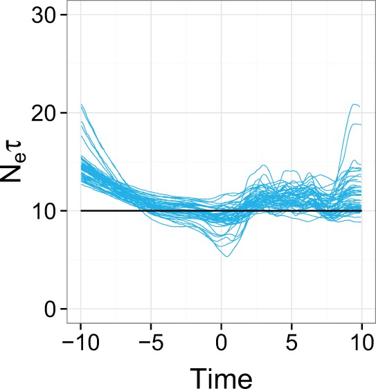
Overlaid median lines of reconstructed skygrid plots for 50 replicates of the uniform temporal sampling scheme in Scenario 1. The black line is the true population size.

The percent bias is the same without the modulus:

$$100\times \frac{1}{R}{\displaystyle {\int }_0^R\frac{\widehat{N}(t)-N(t)}{N(t)}}dt.$$

A negative value of this statistic represents a reconstruction in which the median line of the reconstruction is most often beneath the curve representing the true dynamics, while a positive value represents one in which is it most often above it.

It can, however, be argued that bias in a skyline-family reconstruction is not of great concern. The exact numerical EPS estimates are very difficult to interpret and researchers rarely attempt to do so, instead interpreting the variation in these estimates as representing past demographic variation. As a result, we also calculated an adjusted percent error statistic, which is the percent error once bias has been eliminated. This was determining, for each single analysis, by estimating the constant K which minimizes the absolute value of the percent bias in the function $\widehat{N}(t)+K$, and then using this K to calculate the percent error of $\widehat{N}(t)+K$.

Finally, HPD size is a measure of the precision of the reconstruction:

$$\frac{1}{R}{\displaystyle {\int }_0^R\frac{|{\widehat{N}}_{97.5}(t)-{\widehat{N}}_{2.5}(t)|}{N(t)}}dt,$$

with larger values reflecting wider credible intervals.

The values of these four statistics were calculated for the MCMC analysis that had been performed on every separate replicate of each sampling scheme. The results were then used as the basis for a kernel density estimate (KDE) for the probability density function of each statistic for each sampling scheme. These used a Gaussian kernel and bandwidth picked using the Sheather and Jones (1991) method. For Scenarios 2–5, distributions were then compared by estimation of the coefficient of overlapping, using the OVL₅ estimator described by Schmid and Schmidt (2006). This estimates the area shared by both distributions, ranging from 0 if they have entirely disjoint support and 1 if they are identical. Hypothesis tests were also employed to check whether features of the KDEs and hence coefficients of overlapping were likely to be simply due to chance; as we felt it unwise to make assumptions about the distribution of these statistics, we used non-parametric tests. With so little prior research to base hypotheses on, a post-hoc testing strategy was employed, with the Nemenyi test identifying pairs of sampling schemes for which there was evidence that the distribution of each statistic was different. Test statistic calculations were conducted using the Tukey–Kramer method.

2.5 Marginal likelihood estimation

The only sampling scheme that was employed in analysing Scenario 1 was uniform temporal sampling. While in every other scenario the intention was to compare the performance of different schemes, here we had two other objectives. The first was to determine whether, if spurious (non-constant) dynamics were reconstructed by the skygrid as a result of the particular set of samples selected for analysis, this stochastic sampling effect might be accepted as genuine using formal hypothesis tests. For reasons of computational time, this investigation was restricted to the five sampling replicates whose skygrid reconstructions showed the highest percent error. We perform a formal model comparison between the skygrid (which allows for population dynamics that are not governed by any deterministic function) and a model of constant population size (which should, in this case, be sufficient as it represents the true dynamics). The sequences from the five replicates were re-analysed, replacing the skygrid tree prior with the constant model, and both models were compared by calculating marginal likelihood estimates (MLEs) using both path sampling and stepping-stone sampling (Baele et al. 2013). Ratios of the MLEs were calculated to give a Bayes Factor (BF) comparing the two models.

2.6 Sample size

The second objective in investigating Scenario 1 concerned the size of the sample. For the extra datasets of varying size generated under this scenario, we used weighted least-squares regression (Galecki and Burzykowski 2013) to fit curves for the relationship between adjusted percent error and sample size, and HPD size and sample size. The values of these statistics suggested the possibility of heteroscedasticity, so an assumption of constant variance was not made. The general form of these models for a statistic s of an analysis replicate of sample size n is $g(s)=Af(n)+B+\mathrm{ϵ}$, where f and g are functions, A and B are constants, and ϵ is normally distributed with mean 0 and variance ${\sigma }^2{v}^2(n)$ with v a positive function and ${\sigma }^2$ a scaling factor. A, B, ${\sigma }^2$, and the parameters of v(n) are fit by the regression procedure. For g and f, we considered a linear relationship $s=An+B+\mathrm{ϵ}$, a logarithmic relationship $s=A\text{ln}(n)+B+\mathrm{ϵ}$, a reciprocal relationship $s=\frac{A}{n}+B+\mathrm{ϵ}$, an exponential relationship $\text{ln}(s)=An+B+\mathrm{ϵ}$, and a power law relationship $\text{ln}(s)=A\text{ln}(n)+B+\mathrm{ϵ}$. For the unscaled standard deviation v(n), we considered a null model (such that the variance of estimates was not affected by sample size), an exponential relationship $v(n)=e^{tn}$, a power law relationship $v(n)=|n{|}^t$, and a power law plus constant $v(n)=t_1+|n{|}^{t_2}$, where t, t_1, and t₂ are constants. Modelled relationships were compared with each other using sample-size corrected Akaike information criterion (AICc); where the response variable was transformed, AICc values were corrected appropriately by the addition of the log of the Jacobian determinant of the transformation matrix. The model with the lowest AICc was taken to be the most appropriate.

3. Results

3.1 Skygrid reconstruction

3.1.1 Scenario 1: single population, constant size.

Fig. 2 overlays the median lines for the reconstructions for all fifty replicates of the uniform temporal scheme, with the red line representing the true dynamics. Two observations are immediate: the universal departure of each median line from the true line in the period prior to sampling (which also occurred in every other scenario and is the reason that we concentrated on evaluating the performance of the reconstruction during the sampling period only) and that there is a clear bias towards overestimating population sizes. Fig. 3 displays KDEs for the distribution of each of the four statistics. The performance of the skygrid in reconstructing the true dynamics is variable, even when the samples are chosen according to different replicates of the same scheme; this can be seen in Fig. 4, which shows all reconstructed plots from the analyses of the fifty replicates of the sampling scheme sorted in order of increasing percent error. The best reconstructions are nearly flawless, whereas the worst have spurious features that might lead an unwary researcher to the wrong conclusions. However, the line representing the true EPS does lie within the 95 per cent HPD interval for the entire length of the sampling period in the considerable majority of replicates, and it also always lies within the interval in the period prior to sampling, despite the curve of the median line.

Figure 3.

KDEs for the distribution of statistics indicating the accuracy and precision of the skygrid reconstructions in Scenario 1.

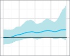
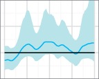
Figure 4.

Skygrid reconstructions for the 50 replicates of the uniform sampling scheme in Scenario 1, sorted by increasing percent error. The black line is the true EPS, the dark blue line the median estimate, and the 95 per cent HPD region is in light blue.

The results of the MLE investigation of the worst five reconstructions (the bottom line in Fig. 4) are summarized in Table 1. BFs greater than 1 support the skygrid over the constant model. In two cases, the constant model is favoured by both estimation methods. In one, it is favoured by stepping-stone sampling, but the skygrid is slightly preferred by path sampling; nevertheless, the BF is only slightly greater than 1 and this would not be interpreted as conclusive. However, the last two replicates give figures that would support the rejection of a constant size population model in favour of more complex dynamics. These dynamics are purely a sampling artefact. In particular, for the replicate with the highest error of all (bottom right, Fig. 4), the difference is dramatic and the hypothesis of constant size would, with no knowledge of the true situation, be decisively rejected.

Table 1.

Results of marginal likelihood estimation.

Skygrid graph	Path sampling			Stepping-stone sampling
	log MLE (Constant)	log MLE (Skygrid)	BF	log MLE (Constant)	log MLE (Skygrid)	BF
	−6,012.19	−6,012.22	0.97	−6,012.63	−6,014.24	0.20
	−5,780.95	−5,782.16	0.30	−5,782.33	−5,784.48	0.12
	−5,665.63	−5,655.55	1.08	−5,655.48	−5,656.52	0.35
	−5,783.08	−5,782.00	2.92	−5,785.65	−5,782.94	15.00
	−5,897.60	−5,892.42	176.81	−5,899.30	−5,893.56	310.21

The five replicates of the uniform sampling scheme, Scenario 1, whose reconstructed skygrid plots had highest percent error in the median line were re-analysed using both the skygrid and a constant population size coalescent model as tree priors. Figures given are the log marginal likelihoods for both priors, estimated using both path sampling and stepping-stone sampling. The BFs given are for the hypothesis that the skygrid model fits the data better than the constant population model.

Fig. 5 displays scatter plots for the adjusted percent error and HPD size statistics against sample size, together with curves representing the fitted models. The model e(n) of adjusted percent error as a function of sample size n with the lowest AICc was a power law relationship, given by:

$$e(n)=4.03\times n^{-0.329}\times \text{exp}({\mathrm{ϵ}}_e),$$

Figure 5.

Scatter plots depicting the relationship between sample size and statistics used to evaluate the performance of the skygrid reconstruction for 100 replicates of the uniform sampling scheme in Scenario 1. The red line represents the best-fit model determined by weighted least squares regression and corrected Akaike information criterion and the grey lines the limit of the 95 per cent confidence interval given by the fitted values of the error term of this model. (a) plots adjusted percent error against sample size and (b) HPD size against sample size.

where ϵ_e has mean 0 and standard deviation $0.668\times \text{exp}(-7.95\times {10}^{-4}\times n)$. The preferred model s(n) of HPD size was also given by a power law:

$$s(n)=12.5\times n^{-0.472}\times \text{exp}({\mathrm{ϵ}}_s),$$

where ϵ_s has mean 0 and standard deviation $21.9\times (n^{-1.11}+5.11\times {10}^{-3})$. The red curves in Fig. 5 are the fitted relationships when the error terms ϵ_e and ϵ_s are equal to zero, and the grey curves the boundaries of the 95 per cent confidence interval according to those error terms. For full tables of AICc scores, and the reconstructed plot from the analysis of every replicate, see the Supplementary Material.

3.1.2 Scenario 2: single population, oscillations.

Fig. 6 displays KDEs for each of the four statistics, with each colour representing a different temporal sampling scheme. The suggestion here is that uniform sampling performs best in each case; even in cases where the distribution of statistics for another scheme has a similar mode, it has a longer tail. The estimated coefficients of overlapping of these KDEs and results of the post-hoc tests comparing results are listed in Table 2. (The OVL₅ estimator has a known tendency to underestimate overlap when the true value is greater than around 0.8 (Schmid and Schmidt 2006), which may be the case in some comparisons here.) While there is considerable overlap (>0.6 in every case) between each pair of distributions, the test results do suggest evidence for a difference between uniform and proportional sampling, which is in favour of the former, at the P < 0.05 level for all four statistics, and also between uniform and reciprocal-proportional sampling (also in favour of the former) for HPD size only. Plots of overlaid median lines for every reconstruction in this scenario and every subsequent one can be found in the Supplementary Material.

Figure 6.

KDEs for the distribution of statistics indicating the accuracy and precision of the skygrid reconstructions in Scenario 2. Distributions are coloured by sampling scheme.

Table 2.

Estimated coefficients of overlapping for distributions of statistics in Scenario 2.

Statistic	Scheme 1	Scheme 2
		Reciprocal-proportional	Uniform
Percent error	Uniform	0.8 (0.289)
	Proportional	0.7 (0.0699)	0.62 ($6.06\times {10}^{-4}$)
Percent bias	Uniform	0.76 (0.166)
	Proportional	0.76 (0.807)	0.76 (0.0395)
Adjusted percent error	Uniform	0.76 (0.0763)
	Proportional	0.74 (0.792)	0.78 (0.0132)
HPD size	Uniform	0.68 ($2.12\times {10}^{-3}$)
	Proportional	0.72 (0.984)	0.7 ($3.87\times {10}^{-3}$)

Each entry in each table compares a statistic between two sampling schemes. Numbers in parentheses are P values from post-hoc (Nemenyi) tests for the null hypothesis that the data used to estimate each KDE came from the same distribution, where these are <0.05 the coefficient of overlapping is given in boldface.

3.1.3 Scenario 3: structured population, constant size.

Fig. 7 displays the KDEs for each statistic. (Note that in this case, the proportionality or reciprocal-proportionality refers to spatial sampling; as the overall population size was constant, we used uniform temporal sampling.) For coefficients of overlapping and results of post-hoc tests, see Table 3. The performance of the uniform and proportional schemes are basically equivalent, but reciprocal-proportional sampling is very different: it is no more accurate, but the bias occurs in the opposite direction. It also gives slightly more precise reconstructions than the other two. Once bias is accounted for, there is no suggestion that the three schemes differ in accuracy.

Figure 7.

KDEs for the distribution of statistics indicating the accuracy and precision of the skygrid reconstructions in Scenario 3. Distributions are coloured by sampling scheme.

Table 3.

Estimated coefficients of overlapping for distributions of statistics in Scenario 2.

Statistic	Scheme 1	Scheme 2
		Reciprocal-proportional	Uniform
Percent error	Uniform	0.78 (0.935)
	Proportional	0.84 (0.671)	0.98 (0.87)
Percent bias	Uniform	0.44 ($2.6\times {10}^{-11}$)
	Proportional	0.22 ($4.8\times {10}^{-14}$)	0.76 (0.504)
Adjusted percent error	Uniform	0.8 (0.178)
	Proportional	0.74 (0.74)	0.78 (0.554)
HPD size	Uniform	0.64 ($4.61\times {10}^{-4}$)
	Proportional	0.54 ($9.18\times {10}^{-6}$)	0.9 (0.649)

Each entry in each table compares a statistic between two sampling schemes. Numbers in parentheses are P values from post-hoc (Nemenyi) tests for the null hypothesis that the data used to estimate each KDE came from the same distribution, where these are <0.05 the coefficient of overlapping is given in boldface.

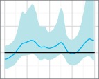
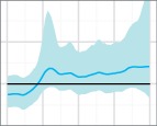
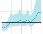
This is the scenario in which the effect of oversampling a single deme towards the end of the timeline was investigated. (The 250 sequences in these analyses that were not part of the oversampling were selected using reciprocal-proportional spatial sampling, as this was marginally the best-performing scheme.) When overlaying the plots (Fig. 8), a spurious bottleneck effect is immediately clear, and it is more extreme if the oversampled deme is smaller. The true value of $N_{\text{e}}\tau$ was outside the 95 per cent HPD interval at the very end of the timeline in 100 per cent of replicates where the oversampled deme was small, 98 per cent where it was medium-sized, and 60 per cent where it was large.

Figure 8.

Overlaid median lines of 50 reconstructed skygrid plots for Scenario 5, where additional samples are selected from one deme in the last 0.25 years of the timeline. The black line is the true population size. Plot titles refer to the oversampled deme and its size.

3.1.4 Scenario 4: structured population, oscillations.

For analyses of this dataset, the default $\text{Gamma}(0.001,0.001)$ prior on the precision parameter of the skygrid was replaced by a more informative $\text{Gamma}(0.1,0.1)$ distribution. This was because, if this was not done, there was a tendency for the skygrid reconstructions to be smoothed such that the median line was virtually flat and no oscillatory behaviour was discernible by eye. This behaviour was accompanied by high posterior estimates for the precision parameter, so the prior was adjusted to place much more weight on low values.

Fig. 9 compares KDEs for different temporal sampling schemes for the same spatial sampling scheme; Fig. 10 does the opposite. The full 9 × 9 tables comparing different schemes by overlapping coefficient and post-hoc tests can be seen in Supplementary Table S3 of the Supplementary Material; the key points are summarized here.

Figure 9.

KDEs for the distribution of statistics indicating the accuracy and precision of the skygrid reconstructions in Scenario 4. Each graph plots the distributions of each statistic for several temporal sampling schemes when the spatial sampling scheme is fixed.

Figure 10.

KDEs for the distribution of statistics indicating the accuracy and precision of the skygrid reconstructions in Scenario 4. Each graph plots the distributions of each statistic for several spatial sampling schemes when the temporal sampling scheme is fixed.

A reciprocal-proportional temporal scheme outperformed a proportional scheme (for the same spatial scheme) in every statistic. For percent error, the largest overlapping coefficient was 0.3 ($P=1.56\times {10}^{-13}$), for percent bias 0.38 ($1.58\times {10}^{-6}$), for adjusted percent error 0.56 ($2.68\times {10}^{-9}$), and for HPD size 0.68 (0.0314). A uniform temporal scheme always outperformed a proportional scheme in three statistics, with maximum coefficients of 0.56 ($3.93\times {10}^{-5}$) for percent error, 0.64 (0.0226) for percent bias, and 0.68 ($2.48\times {10}^{-3}$) for adjusted percent error; for HPD size, evidence for superior precision only existed at the 0.05 level when the spatial scheme was uniform. While the KDE graphs for error and bias suggest that reciprocal-proportional sampling is superior to uniform, in most cases there was insufficient evidence that this difference was genuine, and there is no suggestion of it at all for adjusted error or HPD size.

When spatial sampling schemes were compared for the same temporal scheme, there was no suggestion at all of a difference in performance with regard to percent error, but reciprocal-proportional sampling was clearly less biased, with a maximum overlapping coefficient of 0.36 ($7.63\times {10}^{-7}$) when compared to a proportional scheme or 0.42 ($7.89\times {10}^{-6}$) to a uniform scheme. There was no evidence of any difference between the uniform and proportional schemes. There was also generally little evidence of the superiority of any scheme to any other in regard to adjusted error, but the KDE graphs do suggest that the reciprocal-proportional scheme is in fact worse than the other two in this case and there was some evidence for this when the temporal sampling scheme was itself reciprocal-proportional. For HPD size, again the reciprocal-proportional scheme was more precise; the maximum coefficient was 0.65 ($2.3\times {10}^{-5}$) when comparing to a proportional scheme and 0.64 (0.0145) when comparing to a uniform. There was no evidence of a difference in precision when comparing proportional and uniform schemes.

3.1.5 Scenario 5: structured population, oscillations, out of phase.

The total population size being constant through time in this scenario, we varied only the spatial sampling scheme. In contrast to any other scenario examined here, the bias is universally towards underestimating sizes (Fig. 11). Notably, this bias is most serious for the reciprocal-proportional scheme.

Figure 11.

KDEs for the distribution of statistics indicating the accuracy and precision of the skygrid reconstructions in Scenario 5. Distributions are coloured by sampling scheme.

The final set of coefficients of overlapping and post-hoc test P values are given in Table 4. There is very little to separate the uniform and proportional schemes, but the poor performance of reciprocal-proportional sampling is evident. Superior performance for the uniform scheme over the reciprocal-proportional scheme is also indicated at the 0.05 level for adjusted error, but the difference appears slight as there is considerable overlap in the KDEs. The reciprocal-proportional scheme also retains the superior precision found in other scenarios.

Table 4.

Estimated coefficients of overlapping for distributions of statistics in Scenario 5.

Statistic	Scheme 1	Scheme 2
		Reciprocal-proportional	Uniform
Percent error	Uniform	0.14 ($5.04\times {10}^{-14}$)
	Proportional	0.06 ($2.23\times {10}^{-14}$)	0.8 (0.607)
Percent bias	Uniform	0.18 ($7.28\times {10}^{-14}$)
	Proportional	0.06 ($3.73\times {10}^{-14}$)	0.82 (0.31)
Adjusted percent error	Uniform	0.84 (0.022)
	Proportional	0.84 (0.297)	0.78 (0.476)
HPD size	Uniform	0.64 ($6.62\times {10}^{-3}$)
	Proportional	0.52 ($2.51\times {10}^{-6}$)	0.8 (0.144)

Each entry in each table compares a statistic between two sampling schemes. Numbers in parentheses are P values from post-hoc (Nemenyi) tests for the null hypothesis that the data used to estimate each KDE came from the same distribution, where these are <0.05 the coefficient of overlapping is given in boldface.

4. Discussion

The simulation exercise described here is a more comprehensive effort than any previously published to investigate the effects that sampling schemes have on the reconstruction of the temporal dynamics of viral (or other pathogen) populations from nucleotide sequences. Caution must be taken in generalizing the results here. The range of demographic scenarios that could be simulated is effectively limitless and covering every possible complication or nuance is not feasible. We also assumed a simple, and invariant, mutation model. If demes are taken to be geographical locations, it is also a great simplification to model this under a structured coalescent by assuming that all lineages within each area mix freely. Researchers wishing to investigate sampling effects in a situation analogous to a particular study that they are conducting may wish to design similar simulations with population structures that are more appropriate for their work. Nevertheless, there are several results of this analysis which should inform sampling strategies in general.

We made the choice to analyse multiple replicates of sampling schemes drawing from the same pool of sequences, rather than taking the approach of previous work (Chikhi et al. 2010; Heller, Chikhi, and Siegismund 2013) in which separate coalescent simulations were performed from the same collection of tips; in that situation every sampling ‘replicate’ actually has a unique phylogenetic tree. We feel that our approach is more reflective of the process of devising an actual scheme in the real world, and it also added an element of stochastic variation in the process of sample collection. A drawback is that each master set is a unique stochastic realization of the coalescent simulation, and as a result, some features may be unique only to that realization. Nevertheless, each of the five scenarios considered here used a different master set, and many of the phenomena noted are consistent across them.

It is certainly concerning that stochastic variation in the sequences picked by a sensible sampling scheme can nonetheless introduce spurious temporal variation in skygrid reconstructions, to the extent that hypothesis tests can actually reject an accurate simple model in favour of a more complicated one, although the latter phenomenon was basically absent in three of the five examples tested and only overwhelming in one, which is in all probability an outlier. We make two recommendations as a result of this. The first is that the behaviour of the median line in a plot from the Bayesian skyline family should be regarded with scepticism, and certainly the HPD region must be taken into account. For example, the median lines of the bottom five graphs in Fig. 4 could lead an unwary researcher to suggest many potentially interesting historical scenarios, all of which would in fact be entirely sampling artefacts. But in all but two plots in that figure, a straight line representing an invariant EPS could be drawn through the HPD bounds over the entire extent of the graph. The second recommendation, especially when using a random procedure to downsample large datasets of sequences collected in the past, is to compare the results of analyses from more than one replicate of the scheme, in case any distinctive features of the reconstruction are no more than the results of the samples chosen. While the reconstruction of truly misleading features for this reason does appear to be rare, the possibility should not be ignored.

An alternative to re-running analyses with different sets of sequences would be to include more sequences in the first place, but the results here suggest diminishing gains in accuracy and precision as the sample size increases, which must be weighed against the extra computational time required to analyse a larger dataset. While there are clear advantages in moving from, for example, 25 to 100 sequences, moving from 425 to 500 will have limited impact. The indiscriminate addition of extra sequences without reference to their time and place of origin may also do more harm than good by introducing spurious dynamics to the reconstruction.

One practice that certainly should not continue is the presentation of demographic reconstructions based on datasets consisting disproportionately of a collection of recent isolates taken from the same area. This clearly introduces a spurious bottleneck effect. While this observation is not entirely new (Chikhi et al. 2010; Heller, Chikhi, and Siegismund 2013), it has only been previously shown in situations where all tips in the tree are contemporaneous, and where some demes are entirely unrepresented in the data, and those papers have rarely been cited in the viral phylogenetics literature; here, we have confirmed that it does also hold when tips are distributed over a wider time period and all demes are (unevenly) represented.

The bias towards overestimating EPSs, even in Scenario 1, is unexpected, as the original Bayesian skyline has been shown to be unbiased as an estimator of the harmonic mean of the EPS on an interval (Pybus, Rambaut, and Harvey 2000). It transpires that this is the result of the process of simulating large trees under a particular demographic model and then taking a small subsample of the tips for analysis, as this does not occur if trees are simulated individually on a smaller set of tips and all sequences are used in the analysis (see Supplementary Section S3 of the Supplementary Text).

The superiority of uniform over proportional temporal sampling was recently confirmed in an article by Karcher et al. (2015); the authors did not address spatial sampling and we show here that the uniform approach is also non-inferior in that case. They also propose a new framework in which the distribution of sampling times is explicitly modelled, as a Poisson process with intensity proportional to the EPS. Along similar lines, Volz and Frost (2014) proposed a means by which the coalescent can be augmented with a model of the sampling process, and the birth–death family of tree priors, which replace the coalescent with a forwards-time epidemiological model of transmission, also explicitly account for sampling (Stadler et al. 2011, 2013; Kühnert et al. 2014; Leventhal et al. 2014). Nevertheless, these papers all make the assumption that the sampling process is both known and relatively simplistic. Sampling in the real world is complex and will defy such simple rules; caution should be taken in making a blanket assumption that they hold. This is particularly true when dealing with historical data from the era before methodological sequencing was even contemplated; while it may now be possible to design studies with sampling schemes that mirror the model to be used in the analysis, this is certainly not how isolates were chosen for sequencing in the past. As a result, we argue for uniform sampling as a recommendation for best practice in the most general case. It is also, happily, by far the easiest scheme to design, especially given the complicated relationship between the EPS and disease dynamics (Volz et al. 2009; Frost and Volz 2010; Volz 2012). In more standard epidemiological terminology, uniform sampling is stratification by time period and location. We would caution, however, that a uniform sampling scheme must be carefully designed lest it become effectively proportional. This would occur, for example, if one stratified by year for a pathogen causing disease with a strong seasonal aspect; a random selection from a year’s worth of influenza samples will probably result in a set in which most come from the winter. Care must therefore be taken not to select too wide a time window.

Reciprocal-proportional sampling, unexpectedly, performed as well as uniform sampling in terms of (unadjusted) error and bias in every scenario except 5, and in some cases the suggestion is that it is actually superior. When comparing spatial schemes, it also performs better in regard to HPD size. This finding, which might suggest that the best strategy would be to include epidemiologically rare isolates at a greater frequency than more common ones, should be interpreted with caution, as it is likely that this scheme simply mitigates an existing bias. While in the first four scenarios, the tendency towards overall overestimation of EPSes is present, in Scenario 5 all schemes result in underestimation, with reciprocal-proportional sampling showing the greatest bias in this direction. Since the reciprocal-proportional scheme oversamples small populations, and this depresses reconstructed population sizes (as is clear from the scheme we used in Scenario 3 where a single deme is oversampled), the effect on error and bias seen in other scenarios is most likely to be just a trade-off between two biases in opposite directions. Reciprocal-proportional sampling notably never outperforms uniform sampling for the adjusted error statistic, where bias has been eliminated, although it is often still better than proportional sampling. The gain in precision, on the other hand, appears to genuine, but this is not sufficient reason to adopt this scheme in of itself.

In the situations simulated here, the skygrid provided a reasonable reconstruction of the dynamics of the total population size even where that population was subdivided. For a constant total size, if one compares Fig. 3 to Fig 7 or Fig. 11, there is no obvious difference between the distribution of the percent error or adjusted percent error statistics in the reconstructions of Scenario 1 and Scenario 3 (regardless of sampling scheme) or Scenario 5 (except for reciprocal-proportional sampling). For an oscillating total size, on the other hand, when comparing Fig. 6 to Fig 11, there was rather more error in all reconstructions in Scenario 5 compared to Scenario 2, but the difference is still not massive. Nevertheless, a biasing effect of population structure has been noted before (Heller, Chikhi, and Siegismund 2013) and the extent to which it occurs is likely a consequence of the relative values of the coalescence and migration rates, which we did not vary here. There is scope for further work attempting to identify situations in which this is likely to be a problem.

Ideally, population structure would be accounted for by the use of a model that is aware of it; while publicly available methods of this type currently do not allow for changes in deme sizes over time (Vaughan et al. 2014; De Maio et al. 2015), we anticipate that this may change in future. An alternative approach would be to perform separate analyses on the sequences in each deme, although since this ignores the possibility of migration, it is also a simplification and is most suitable for situations where between-deme movements are not common.

To conclude, we would make four recommendations as the result of this study. First, since the variation in population sizes reconstructed by Bayesian skyline family methods can be subject to spurious phenomena caused by nothing more than the choice of samples, it would be preferable if researchers were to repeat analyses with different sample sets. Second, the behaviour of the median line of a skyline family plot should not be overinterpreted if the HPD region would support several alternative interpretations. Third, when selecting past sequences to use from an uneven set of samples, or as a baseline methodology in the design of future studies, sequence selection should be stratified by time period and location, without reference to the size of the pathogen population, or number of infections, at that location or during that period. Finally, we advise against the disproportionate inclusion of a large amount of sequence data from a single location, as this introduces false dynamics which should not be interpreted as a genuine decline in the size of viral populations.

Data availability

Data (complete simulated sequence datasets, XML files for BEAST, and data used to generate KDEs) are made available as part of the Supplementary Material.

Supplementary data

Supplementary data are available at Virus Evolution online.

References

- Baele G., et al. (2013) ‘Accurate Model Selection of Relaxed Molecular Clocks in Bayesian Phylogenetics’, Molecular Biology and Evolution, 30: 239–43. [DOI] [PMC free article] [PubMed] [Google Scholar]
- Bielejec F., et al. (2014) ‘πBUSS: A Parallel BEAST/BEAGLE Utility for Sequence Simulation Under Complex Evolutionary Scenarios’, BMC Bioinformatics, 15: 133. [DOI] [PMC free article] [PubMed] [Google Scholar]
- Chikhi L., et al. (2010). ‘The Confounding Effects of Population Structure, Genetic Diversity and the Sampling Scheme on the Detection and Quantification of Population Size Changes’, Genetics, 186: 983–95. [DOI] [PMC free article] [PubMed] [Google Scholar]
- De Maio N., et al. (2015) ‘New Routes to Phylogeography: A Bayesian Structured Coalescent Approximation’, PLoS Genetics, 11: e1005421. [DOI] [PMC free article] [PubMed] [Google Scholar]
- de Silva E., Ferguson N. M., Fraser C. (2012) ‘Inferring Pandemic Growth Rates from Sequence Data’, Journal of The Royal Society Interface, 9: 1797–808. [DOI] [PMC free article] [PubMed] [Google Scholar]
- Drummond A. J., et al. (2005) ‘Bayesian Coalescent Inference of Past Population Dynamics from Molecular Sequences’, Molecular Biology and Evolution, 22: 1185–92. [DOI] [PubMed] [Google Scholar]
- Drummond A. J., et al. (2012) ‘Bayesian Phylogenetics with BEAUti and the BEAST 1.7’, Molecular Biology and Evolution, 29: 1969–73. [DOI] [PMC free article] [PubMed] [Google Scholar]
- Frost S. D. W., Volz E. M. (2010) ‘Viral Phylodynamics and the Search for an ‘Effective Number of Infections’’, Philosophical Transactions of the Royal Society of London B Biological Sciences, 365: 1879–90. [DOI] [PMC free article] [PubMed] [Google Scholar]
- Frost S. D. W., et al. (2015) ‘Eight Challenges in Phylodynamic Inference’, Epidemics, 10: 88–92. [DOI] [PMC free article] [PubMed] [Google Scholar]
- Galecki A., Burzykowski T. (2013) Linear Mixed-Effects Models Using R: A Step-by-Step Approach, English. 2013 edn. New York: Springer. [Google Scholar]
- Gill M. S., et al. (2013) ‘Improving Bayesian Population Dynamics Inference: A Coalescent-Based Model for Multiple Loci’, Molecular Biology and Evolution, 30: 713–24. [DOI] [PMC free article] [PubMed] [Google Scholar]
- Hall M. D., et al. (2013) ‘Reconstructing Geographical Movements and Host Species Transitions of Foot-and-Mouth Disease Virus Serotype SAT 2’, mBio, 4: e00591–13. [DOI] [PMC free article] [PubMed] [Google Scholar]
- Hasegawa M., Kishino H., Yano T. A. (1985) ‘Dating of the Human-Ape Splitting by a Molecular Clock of Mitochondrial DNA’, Journal of Molecular Evolution, 22: 160–74. [DOI] [PubMed] [Google Scholar]
- Heller R., Chikhi L., Siegismund H. R. (2013) ‘The Confounding Effect of Population Structure on Bayesian Skyline Plot Inferences of Demographic History’, PLoS One, 8: e62992. [DOI] [PMC free article] [PubMed] [Google Scholar]
- Karcher M. D., et al. (2015) ‘Quantifying and Mitigating the Effect of Preferential Sampling on Phylodynamic Inference’, arXiv:1510.00775 [q-bio, stat]. arXiv: 1510.00775. [DOI] [PMC free article] [PubMed] [Google Scholar]
- Kühnert D., et al. (2014) ‘Simultaneous Reconstruction of Evolutionary History and Epidemiological Dynamics from Viral Sequences with the Birth–Death SIR Model’, Journal of the Royal Society Interface, 11: 20131106. [DOI] [PMC free article] [PubMed] [Google Scholar]
- Leventhal G. E., et al. (2014) ‘Using an Epidemiological Model for Phylogenetic Inference Reveals Density Dependence in HIV Transmission’, Molecular Biology and Evolution, 31: 6–17. [DOI] [PMC free article] [PubMed] [Google Scholar]
- Lin J.-H., et al. (2011) ‘Phylodynamics and Molecular Evolution of Influenza A Virus Nucleoprotein Genes in Taiwan Between 1979 and 2009’, PLoS One, 6: e23454. [DOI] [PMC free article] [PubMed] [Google Scholar]
- Minin V. N., Bloomquist E. W., Suchard M. A. (2008) ‘Smooth Skyride Through a Rough Skyline: Bayesian Coalescent-Based Inference of Population Dynamics’, Molecular Biology and Evolution, 25: 1459–71. [DOI] [PMC free article] [PubMed] [Google Scholar]
- Notohara M. (1990) ‘The Coalescent and the Genealogical Process in Geographically Structured Population’, Journal of Mathematical Biology, 29: 59–75. [DOI] [PubMed] [Google Scholar]
- Padhi A., Ma L. (2014) ‘Genetic and Epidemiological Insights into the Emergence of Peste Des Petits Ruminants Virus (PPRV) Across Asia and Africa’, Scientific Reports, 4: 7040. [DOI] [PMC free article] [PubMed] [Google Scholar]
- Phillips J. E., et al. (2014) ‘Evolutionary Dynamics of West Nile Virus in Georgia, 2001–2011’, Virus Genes, 49: 132–6. [DOI] [PubMed] [Google Scholar]
- Pybus O. G., Rambaut A., Harvey P. H. (2000) ‘An Integrated Framework for the Inference of Viral Population History from Reconstructed Genealogies’, Genetics, 155: 1429–37. [DOI] [PMC free article] [PubMed] [Google Scholar]
- Schmid F., Schmidt A. (2006) ‘Nonparametric Estimation of the Coefficient of Overlapping—Theory and Empirical Application’, Computational Statistics and Data Analysis, 50: 1583–96. [Google Scholar]
- Sheather S. J., Jones M. C. (1991) ‘A Reliable Data-Based Bandwidth Selection Method for Kernel Density Estimation’, Journal of the Royal Statistical Society Series B (Methodological), 53: 683–90. [Google Scholar]
- Stack J. C., et al. (2010) ‘Protocols for Sampling Viral Sequences to Study Epidemic Dynamics’, Journal of the Royal Society Interface, 7: 1119–27. [DOI] [PMC free article] [PubMed] [Google Scholar]
- Stadler T., et al. (2011) ‘Estimating the Basic Reproductive Number from Viral Sequence Data’, Molecular Biology and Evolution, 29: 347–57. [DOI] [PubMed] [Google Scholar]
- Stadler T., et al. (2013) ‘Birth-Death Skyline Plot Reveals Temporal Changes of Epidemic Spread in HIV and Hepatitis C Virus (HCV)’, Proceedings of the National Academy of Sciences of the United States of America, 110: 228–33. [DOI] [PMC free article] [PubMed] [Google Scholar]
- Vaughan T. G., et al. (2014) ‘Efficient Bayesian Inference Under the Structured Coalescent’, Bioinformatics, 30: 2272–9. [DOI] [PMC free article] [PubMed] [Google Scholar]
- Volz E. M. (2012) ‘Complex Population Dynamics and the Coalescent Under Neutrality’, Genetics, 190: 187–201. [DOI] [PMC free article] [PubMed] [Google Scholar]
- Volz E. M., Frost S. D. W. (2014) ‘Sampling Through Time and Phylodynamic Inference with Coalescent and Birth–Death Models’, Journal of The Royal Society Interface, 11: 20140945. [DOI] [PMC free article] [PubMed] [Google Scholar]
- Volz E. M., et al. (2009) ‘Phylodynamics of Infectious Disease Epidemics’, Genetics, 183: 1421–30. [DOI] [PMC free article] [PubMed] [Google Scholar]
- Wakeley J. (2008) Coalescent Theory: An Introduction. Greenwood Village, CO: Roberts & Co. [Google Scholar]
Associated Data
This section collects any data citations, data availability statements, or supplementary materials included in this article.
Supplementary Materials
Data Availability Statement