

Abstract
Recent observations of dynamic water systems beneath the Greenland and Antarctic ice sheets have sparked renewed interest in modelling subglacial drainage. The foundations of today's models were laid decades ago, inspired by measurements from mountain glaciers, discovery of the modern ice streams and the study of landscapes evacuated by former ice sheets. Models have progressed from strict adherence to the principles of groundwater flow, to the incorporation of flow ‘elements’ specific to the subglacial environment, to sophisticated two-dimensional representations of interacting distributed and channelized drainage. Although presently in a state of rapid development, subglacial drainage models, when coupled to models of ice flow, are now able to reproduce many of the canonical phenomena that characterize this coupled system. Model calibration remains generally out of reach, whereas widespread application of these models to large problems and real geometries awaits the next level of development.
Keywords: cryosphere, subglacial hydrology, basal processes, hydraulics, hydrological models, glacier and ice-sheet dynamics
1. Introduction
The past decade has seen a proliferation of studies from the Greenland and Antarctic ice sheets that implicate subglacial water in driving rapid ice-flow variations detected many hundreds of metres above at the ice surface. The discovery of filling and draining subglacial lakes in Antarctica [1–3] and their association with persistent fast-flow features [4–6] and transient acceleration [7], along with terrestrial evidence for subglacial flooding [8], has revealed unexpected dynamism in this subglacial system isolated from the surface. In Greenland, measurements of seasonal [9–12] and short-term [13–15] variations in outlet-glacier flow have prompted research into surface-to-bed hydrological coupling [16–18] and the role of surface meltwater in overall ice-sheet dynamics [19–21]. These observations have invigorated the development of new subglacial drainage models. Numerous reviews have been written on glacier hydrology, but most have focused on observational work from temperate [22–24] or polythermal glaciers [25,26]. Others have included treatment of theoretical work [27–29], but the only reviews to address modelling explicitly have focused on surface hydrology and runoff prediction [30,31]. This review addresses drainage-system modelling applicable to ice dynamics, and is motivated by the observations described above as well as recent and significant advances in the models themselves.
2. Background
Water was recognized to play a facilitatory role in glacier flow by some of the earliest pioneers of modern glaciology [32,33] (see Clarke [34]). It was not until the 1960s, 1970s and 1980s, however, that the theoretical foundations for our modern conceptual models of glacier drainage were laid (figure 1). This work focused on the mathematical description of individual elements of the basal drainage system, including water sheets [35–37], cavities formed in the lee of bedrock obstacles [38–41], ice-walled conduits [42,43] and bedrock channels [44]. In some cases, natural experiments in the form of glacier surges [45] or outburst floods [46] furnished data with which to test these models. Alongside observations of ordinary glacier behaviour, these phenomena revealed the dynamic nature of drainage-system morphology in which spatial and temporal transitions between fast/efficient/channelized and slow/inefficient/distributed flow play an important role [47].
Figure 1.

Development of and motivation for spatially distributed models of subglacial drainage. (a) Conceptual diagram of scientific progress from (1) theoretical models of drainage-system ‘elements’ to (4) current multi-element models, plotted qualitatively as a function of model sophistication and spatial dimension. (b) Number of drainage-model publications per year, 1960–2014, partitioned by application to glaciers and icecaps, paleo ice sheets, Antarctica and Greenland.
The first models of glacier hydrology were developed to quantify glacier contribution to the timing and volume of run-off [48–50], and thus to assess the role played by glaciers in the hydrological cycle (see references [27,31,51] for reviews). A separate trajectory of model development was motivated by the recognition that the retention, evacuation and distribution of subglacial water is a fundamental control on glacier and ice-sheet dynamics [52,53], and thus on many interesting phenomena observed at the ice surface. Walder [29] cites Röthlisberger [43] and Shreve [42] as evidence of a transition in glacier hydrology from a subdiscipline of surface hydrology to one of glaciology in its methodology and motivation. Early attempts to model the glacier drainage system for the purpose of informing ice dynamics borrowed principles from groundwater hydrology in treating the subglacial horizon as an aquifer [54,55]. Studies concerned with englacial or subglacial water routing used calculations of fluid potential and flow nets to determine hypothetical water pathways through the glacier system [42,56].
The next generation of models sought more realistic representations of the basal drainage system [57–63], with the ultimate goal of coupling these models to ice dynamics. This led to compromise in the explicit representation of individual drainage elements in some cases, or to restrictive requirements that a pre-existing drainage network be defined in others. Such compromise, however, enabled the first hydrologically coupled ice-flow models to be developed [57,58]. Subsequent work (figure 1a) has attempted a more explicit representation of both fast (i.e. channelized) and slow (i.e. distributed) drainage [64–67], but until recently, these models have been limited to one dimension or lacked realistic transient two-way coupling between the elements (cf. [68,69]).
The latest developments have seen these obstacles overcome through a two-dimensional numerical framework that allows a slow (continuum) drainage system to interact with a network of discrete channels in a manner that permits transient evolution of drainage system morphology [70–72]. This advance makes use of the basic elements of a bedrock-floored drainage system—linked cavities and Röthlisberger channels—but implements them in two dimensions which allows straightforward coupling with iceflow models. These models have been developed for application to mountain glaciers and the margins of the Greenland ice sheet (figure 1b), where conditions permit access of surface melt-water to a bed that is often assumed rigid and impermeable (‘hard beds’ in the glaciological lexicon). A largely separate strand of research, inspired by the glacial deposits of former ice sheets and evidence for deformable sediments beneath the modern ice streams, has focused on the hydrology of permeable subglacial sediments (‘soft beds’). Most ‘soft-bed’ hydrology models to date have targeted Antarctica (cf. [73]), with a particular focus on ice-streams [74–80]. Studies of Antarctic basal hydrology are not limited to treating deformable sediment however [81,82], and have recently expanded to include the dynamics of subglacial lakes [83–85].
This review blends chronological and thematic approaches in order to trace the evolution of the discipline, while providing a framework for classifying subglacial drainage models based on methodology and application. It begins with a recipe for drainage models (§3) and a review of theoretical drainage-system ‘elements’ (§4), which form the building blocks of most models. The sections that follow provide an overview of the early models influenced by groundwater hydrology (§5), ‘next-generation’ models aimed at more realistic representation of drainage at the ice–bed interface (§6), models that incorporate multiple drainage elements (§7) and models of Antarctic hydrology (§8). I have chosen to omit a review of the observational basis for these models, as this has been summarized elsewhere for alpine glaciers [23,24,26] and ice sheets [15,86,87]. I have also chosen to focus on spatially distributed models generally aimed at informing ice dynamics, and have thus excluded much important work on jökulhlaups (glacier outburst floods) except where it bears directly on the models discussed herein.
3. Recipe for a subglacial drainage model
Spatially distributed models of glacier drainage require several common ingredients. Conservation of mass gives rise to the continuity equation,
| 3.1 |
written here for an incompressible fluid with an aerially averaged water volume or water depth h (L), water flux q (L2 T−1) and source/sink term b (L T−1). Potential water sources and sinks,
| 3.2 |
arise from melt, rain or runoff from the ice surface bs, water produced through englacial processes such as strain heating be, groundwater recharge/discharge in underlying or adjacent aquifers ba and basal water production or consumption bb. In situ basal water production commonly includes melt due to the geothermal flux Qg/(ρiL) and the frictional heat flux associated with glacier sliding Qf/(ρiL), with ρi the density of ice and L the latent heat of fusion.
Conservation of linear momentum can be used to derive an expression for fluid velocity u, from which flux q can be computed by integrating velocity over flow depth h. More commonly, however, models simply adopt empirical expressions for flux of the following general form:
| 3.3 |
where K is a rate factor, ∇ϕ is the fluid potential gradient and exponents α and β depend on the conceptual model of the drainage system, including whether flow is laminar or turbulent. For α=β=1, (3.3) reduces to Darcy's law for laminar flow, whereas and are typical for turbulent flow through a sheet or cavity system. In its most general form, the rate factor Kij(x,y,z,t) is a tensor field, allowing for both anisotropy and heterogeneity. For pipe-like rather than sheet-like subglacial drainage, an expression for discharge Q (L3 T−1) rather than flux q (L2 T−1) would be used, with a flow cross section S replacing the equivalent flow depth h. In this case, K might be a function of the hydraulic radius and wetted perimeter of the flow element as well as its surface roughness.
The fluid potential ϕ is the total mechanical energy per unit volume of fluid required to move the fluid from one state to another, where the states differ by a pressure pw and an elevation z
| 3.4 |
where ρw is the density of water and g is the gravitational acceleration. Gradients in potential, ∇ϕ, are the primary drivers of water flow. Some models require a relationship between h and pw to close the equations. Other models set ϕ=ρigH+ρwgz, with ice thickness H, such that fluid potential is defined only by ice geometry.
Finally, models that allow the drainage system itself to evolve require additional equations of the form
| 3.5 |
where h′ is a measure of the effective drainage-system capacity, such that h=h′ implies saturation. The opening and closure terms are specific to the conceptual model. Ice-walled conduits are the most common example of evolving drainage elements, where opening is described by melting of the conduit walls and closure by the inward creep of ice.
4. Elements of the basal drainage system
Numerous drainage-system structures have been envisioned over the years (figure 2), inspired primarily by inference based on deglaciated landscapes [88] or measurements of proglacial stream variables, including electrical conductivity [89], concentration of chemical species [90], suspended sediment [91] or injected tracers [45,92,93]. Measurements of subglacial water pressure [94–99], along with the less common measurements of borehole turbidity, electrical properties and geochemistry [100–103], have also been used to study drainage-system structure and dynamics [103–106]. Direct visual observations are rare, though borehole imagery [107,108] and exploration of englacial/subglacial tunnels [109,110] and cavities [111] have furnished some important and surprising information [112].
Figure 2.

Idealized ‘elements’ of the subglacial drainage system as described in the literature. Elements are grouped into those associated with ‘fast’, ‘efficient’ or ‘channelized’ drainage, versus those associated with ‘slow’, ‘inefficient’ or ‘distributed’ drainage. Canals may be classified either way, depending on the relative efficiency of opening and closure processes.
Common to the descriptions of many of the elements is a consideration of (i) the mechanisms of element opening (e.g. by melting of the ice roof, removal of fines from unconsolidated sediment, erosion of bedrock, glacier sliding over bedrock obstacles) and closure (e.g. by ice creep, sediment deformation, freeze-on of supercooled water), (ii) whether water flow through the elements is laminar or turbulent, (iii) the relationship between water discharge and effective pressure and (iv) the stability of the drainage system to perturbations in discharge. Although other reviews describe the elements below (see [28] in particular), they are included here as the basis for most subsequent model development.
(a). Sheets
The water sheet or film was among the first conceptual models of subglacial drainage described in the literature. A lubricating film of water was initially invoked by Weertman [113] as part of his theory of sliding by regelation and enhanced creep around bedrock obstacles. Weertman [35] asserted that ‘catastrophic’ glacier advance was possible if, among other things, the film attained a thickness greater than the height of the obstacles providing the bulk of resistance to sliding by regelation and enhanced creep. Steady-state sheet thickness D was computed by equating the mean flow velocity v of water between two rigid plates and the velocity required to balance the water production rate W (from geothermal and frictional heat flux) under a given hydraulic gradient α:
| 4.1 |
with water viscosity μ, density ρ and distance downglacier x. Nye [44] argued that this film could not both support regelation and convey an appreciable water flux through the subglacial drainage system, suggesting that the regelation film would be of micrometre-scale thickness and that ice- and bedrock channels would convey most water in the drainage system. Using perturbation analysis, Walder [37] concluded that water sheets in excess of several millimetres would grow unstably on planar beds, and thus could not comprise the primary drainage system under realistic conditions. Although undulating beds [44], variable sheet thickness [36,37] and water flow over saturated sediments [75] had already been considered, Creyts & Schoof [114] introduced an extra measure of realism by including partial support of the ice roof by clasts. Stable steady-state sheets are possible in this analysis owing to a negative feedback between sheet thickness and closure rate of the ice roof. Contact area between the ice roof and the supporting clasts diminishes as the water sheet thickens, thus increasing the effective stress on the clasts that remain in contact with the ice. This increase in effective stress drives sheet closure through regelation and creep. Both the prescribed clast sizes and their spatial distribution influence the stability regions of the water sheet, but centimetre- to decimetre-thick sheets are possible if supported by clasts of comparable radii [114].
(b). Channels
Conduits formed partially or entirely within glacier ice represent the canonical ‘fast’ or efficient drainage element. Englacial and subglacial drainage through a three-dimensional channelized system was articulated by Shreve [42], whereas Röthlisberger [43] described the physics of the ice-walled conduits that now bear his name (‘R-channels’). Röthlisberger [43] assumed saturated flow in a circular or semicircular conduit, where the rate of melt opening owing to the viscous dissipation of heat in the flow [115] is balanced by the rate of closure owing to creep of the surrounding ice [116]:
| 4.2 |
and
| 4.3 |
with conduit cross-sectional area S, time t, discharge Q=vS, mean turbulent flow velocity v, densities of ice ρi and water ρw, latent heat of fusion L, gravitational acceleration g, conduit elevation z, flow-following spatial coordinate s, the change in melting temperature with pressure (Clausius–Clapeyron slope) ct, specific heat capacity of water cp, water pressure pw, ice flow-law coefficient A and exponent n=3 and ice overburden pressure pi. The first term in (4.2) represents the conversion of gravitational potential energy into heat available for enlargement of the conduit walls by melting. The second term is the energy contribution from the pressure potential gradient, less the amount required to keep the water at the pressure-dependent melting temperature; this term represents an additional energy source if water flow is in the direction of increasing pressure potential. The constant 1−ctρwcp has a value close to 0.7, thus reducing the total energy available for wall melting by approximately 30% for a flat glacier bed (∂z/∂s=0). By adopting an expression for turbulent pipe flow from hydraulics to describe velocity v, assuming a flat glacier bed and setting (4.2) and (4.3) equal, steady-state channel discharge is found to be weakly but inversely proportional to the pressure gradient:
| 4.4 |
Steeper pressure gradients are thus associated with smaller channels, implying a tendency for large channels to capture water from small ones. This property leads to a positive feedback that makes channels inherently unstable in the presence of an adequate water supply [117]. Under conditions of steady state and for a typical valley glacier geometry, the above would lead to an arborescent drainage system whereby very few large channels are fed by a network of smaller tributaries [42,43].
Broad and low conduits were proposed as more plausible than semicircular R-channels by Hooke et al. [118], who asserted that higher creep closure rates than those predicted by the Röthlisberger model yielded a better match to measurements of basal water pressure. Lliboutry [119] and Hooke [120] challenged the assumption of saturated flow, with Hooke [120] suggesting that unsaturated or air-filled conduits would be common on steep bed slopes and under thin ice according to the discharge condition
| 4.5 |
with ice thickness Z, glacier bed slope β and constant C4, which depends on the ice flow-law coefficient and the assumed channel roughness. The conditions under which channels would be over- or under-full have been explored in a recent holistic analysis of a coupled cavity–conduit drainage system model [121].
The study of jökulhlaups, or glacier outburst floods [46,122], has produced many of the subsequent advances in modelling drainage through subglacial channels. Time-dependence and heat transfer [117,123,124] were two significant additions to the original theory, motivated by an interest in simulating the dynamics and the hydrographs of jökulhlaups [125,126]. Clarke [127] addressed the issues of numerical stiffness in the comprehensive Spring–Hutter formulation to produce a spatially resolved time-dependent model of jökulhlaup propagation. This model demonstrates the inadequacy of assuming a constant and uniform fluid potential gradient along the flowpath, and accounts for advection of heat in the conduit (cf. [117]), producing more plausible values of calibrated channel roughness. Although successful in simulating many aspects of the classical jökulhlaup hydrograph (cf. [64]), current models still overestimate outlet flood-water temperature (see reference [128] for a review), pointing to a persistent shortcoming in the treatment of jökulhlaup thermodynamics [129]. The most sophisticated subglacial drainage models we have still employ the basic concepts and mathematics laid down by Röthlisberger [43] over 40 years ago.
(c). Cavities
Separation of the ice and bed during the sliding process, or cavitation, was considered in the early sliding theory of Lliboutry [38] and incorporated into subsequent work concerned with the relationship between basal sliding and effective pressure [39,130–132], but it was Kamb [41] who is credited with the theoretical description of a system of ‘linked cavities’ that still features widely in the interpretation of basal drainage phenomena. Lliboutry [38] considered the processes of regelation and enhanced creep both with and without cavitation, in the presence of a bed comprising superimposed sinusoidal bumps. He calculated basal water pressures for several limiting cases, suggesting a role for water in governing basal friction and thus sliding speed. Cavity hydraulics were explored theoretically by Walder [40] and cavity pressure–sliding relationships in a numerical model by Iken [39]. Walder [40] considered steady-state water-filled cavities that enlarge by melt opening and glacier sliding, and close by ice creep. By assuming a defined geometry and constant hydraulic gradient, he calculated steady-state cavity length and discharge, showing that (i) cavity pressure increases with discharge, unlike the relationship in R-channels, and cavities are thus stable to perturbations above a threshold effective pressure [39], (ii) cavities become unstable at low effective pressures when creep closure cannot balance cavity opening and (iii) mean water flow speed through cavities is lower than through R-channels of the same cross section under the same hydraulic gradient.
Similar conclusions were reached in the detailed analysis by Kamb [41], where the properties and stability of a linked cavity system were investigated. Such a system was envisioned to form as ice slides over a rough impermeable bed, and was inspired by detailed observations of the 1982–1983 surge of Variegated Glacier [45]. Kamb [41] considers cavities decimetres in height and metres in width, connected by narrow passages (‘orifices’), which accommodate all of the fluid potential drop in the system and ‘throttle’ the flow between cavities. Orifice dynamics, which include melt of the ice roof by viscous dissipation of heat in the flow, opening by glacier sliding and closure by ice creep, therefore hold the key to system behaviour and stability. Adopting two geometrical idealizations of the cavity system, step-like and wave-like bed obstacles, expressions for discharge as a function of effective pressure are derived that confirm a behaviour opposite to that of R-channels: steady-state effective pressure decreases (or water pressure increases) with increasing discharge. This relationship defines one of the key differences between ‘fast’ (e.g. R-channel) and ‘slow’ (e.g. linked cavity) drainage systems, and for step-like orifices is written
| 4.6 |
where N0 is the number of orifices across the width of the glacier, M is the Manning roughness, α is the longitudinal hydraulic gradient, Λ is the head gradient concentration factor, ω is the tortuosity of the system, η is ice viscosity, ν is sliding velocity, σ is effective pressure and ϕ is a flux factor, not to be confused with (3.4). For the same values of hydraulic gradient and discharge, a linked-cavity system has a much greater cross-sectional area and operates at higher basal water pressures than a channel-dominated system. Stability is another key difference between R-channels and linked cavities, as Kamb [41] demonstrates through the orifice melting-stability parameter, here written for a step-like geometry:
| 4.7 |
with D=ρiL/ρwg and the other variables as defined above. The system becomes dominated by viscous heating when Ξ>1 (or Ξ>1.5 for a wave-like geometry), and thus unstable to small perturbations in conduit size or effective pressure. Above these thresholds of Ξ, the cavity system may develop unstably in a manner not dissimilar to R-channel formation. This instability provides a mechanism for a morphological transition from anastomosing (distributed) drainage to arborescent (channelized) drainage, consistent with observations of the termination of the Variegated Glacier surge [45] and numerous observations since [133]. While channels are unstable to infinitesimal perturbations, a linked cavity system is stable over a finite range of perturbations, allowing it to be long-lived particularly in the presence of high sliding rates. Although numerous assumptions were made in the interest of tractability, the basic physics of cavity systems articulated by Kamb [41] have changed little in subsequent model development [70].
(d). Sedimentary canals
Interest in the hydromechanical properties of unconsolidated (‘soft’) glacier beds, prompted by an association between fast ice flow and till deformation [52,134,135], inspired theoretical work on more realistic representations of drainage elements appropriate for soft beds [54,75,136–139]. Shoemaker [54] envisaged a series of parallel channels within a deforming subglacial aquifer that would convey water to the ice-sheet margin, but did not consider the processes of sediment transport and creep that would influence channel shape and evolution. A more detailed consideration of till processes led Alley [137] to conclude that subglacial channels can exist within till sheets, owing to the shear strength and/or viscosity of the till which limits the lateral extent over which creep occurs. Depending on assumed till rheology and other model parameters, creep was found to operate over distances of 5–10 times the till thickness [137].
Walder & Fowler [138] outlined a mathematical description of till-floored and ice-roofed conduits, in which melt opening and ice creep [43] govern the evolution of the conduit roof, and sediment erosion and till creep [140] govern the evolution of the conduit floor. Using a viscous rheology for till [141], they compute a critical effective pressure that separates regimes dominated by ice creep above and till creep below:
| 4.8 |
with subscripts ‘s’ and ‘i’ referring respectively to sediment and ice, densities ρ, conduit perimeters l, conduit-closure shape factors K, ice flow-law parameters A and n, and till flow-law exponents a and b. For plausible values of the above parameters, Walder & Fowler [138] estimate . For effective pressure in the conduit , discharge Q∝N5nc, thus defining an R-channel-dominated regime in which effective pressure increases with discharge. For , a canal-dominated regime exists in which discharge Q∝N−nc. Subsequent calculations suggest that the steeper surface slopes (and thus hydraulic gradients) of alpine glaciers favour R-channel-dominated drainage, while the shallower slopes characteristic of ice sheets favour canal-dominated drainage. Ng [142] refined this model by introducing a more complete treatment of sediment transport and allowing longitudinal variation in model variables. Ng found a tendency for canals to deepen and widen downstream, as well as a dependence of canal effective pressure on sediment discharge: , where Q and Qs are water- and sediment discharge, respectively.
(e). Porous flow
Based on the observation of widespread till deposits of the former ice sheets [143], as well as the discovery of saturated sediment beneath fast-flowing Antarctic ice streams [52], treating the subglacial drainage system as a porous medium [54,55] was a logical early step in drainage modelling. Such descriptions assume laminar flow in which water flux can be described by Darcy's law,
| 4.9 |
written here with dimensions of L T−1 (cf. (3.3)), with hydraulic conductivity K a function of the medium and the fluid, and hydraulic head h=z+Ψ a function of elevation head z and pressure head Ψ=p/ρwg, where p is the water pressure above some reference value p0, usually atmospheric pressure. Hydraulic head is closely related to the potential ϕ in (3.4) as h=ϕ/ρwg. Models typically assume saturated flow, and thus neglect capillary potential along with atmospheric pressure, taking p0=0. The hydraulic conductivity Kij=ρwgkij/μ, a tensor function of material permeability kij and fluid density ρw and viscosity μ, is usually assumed to be homogeneous and isotropic within a given hydrostratigraphic unit. Kij thus becomes a scalar K as in (4.9). The transient groundwater flow equation further requires that porosity and aquifer compressibility be known (here written for a homogeneous isotropic aquifer):
| 4.10 |
with specific storage Ss=ρwg(α+nβ) a function of aquifer porosity n, and the compressibilities of the aquifer α and fluid β.
In models concerned with deformable sediment, hydraulic conductivity K is parametrized to account for its dependence on changes in material porosity through compression and dilatation [144]. The continuum mixture model of Clarke [145] provides a mathematical framework for modelling a deformable subglacial till, including water and sediment transport, water and skeleton compressibility, shear deformation and dilatancy of the till layer and comminution of clasts. Models that couple basal hydrology and sediment deformation typically make use of the Mohr–Coulomb criterion to describe till shear strength τ* as a function of effective pressure N (see [146,147]),
| 4.11 |
with apparent cohesion c0 and friction angle ψ. In these models, till porosity or void ratio is nonlinearly related to shear strength, and therefore effective pressure.
5. Early models from groundwater hydrology
Many of the first models of subglacial drainage imported principles from the more mature discipline of groundwater hydrology (table 1). The motivation for such studies is varied, ranging from understanding basal effective pressure, till deformation and landform development [148,149] to assessing the influence of glaciation and permafrost on groundwater recharge, circulation and geochemistry [150–153]. The first theoretical models were hatched with the Pleistocene ice sheets in mind [144] (figure 3); geographically referenced model applications followed, first to the paleo ice sheets of Europe [154–157] and then North America [151,158–161]. Some of this work has been motivated by the prospective development of deep geologic repositories for nuclear waste [162,163], where the influence of glaciation on subsurface hydrogeology is important in terms of aquifer properties, groundwater geochemistry, saltwater–freshwater interactions and reorganization of groundwater flow (see Person et al. [164] for a review).
Table 1.
Selected models from groundwater hydrology, 1973–1997. Hydraulic conductivity (K), permeability coefficient (k), layer thickness (d), aquifer (af), aquitard (at), basement rock (bsmt), longitudinal coordinate x, transverse coordinate y, vertical coordinate z.
| references | model dimension | model domain | steady-state versus transient | drainage at ice–bed interface? | water sources | key parameters | application |
|---|---|---|---|---|---|---|---|
| Campbell & Rasmussen [49] | one (x) | glacier body | T | no | calculated surface melt | ksnow, kice | South Cascade Glacier (USA) |
| Boulton & Jones [144] | one (x) | deformable subglacial layer | SS | no | prescribed basal melt | Ktill, Kgravel | idealized ice-sheet outlet |
| Shoemaker [54] | one (y) | deformable aquifer over aquitard | SS | prescribed R channels | prescribed basal melt | Kaf, channel spacing | idealized transect |
| Shoemaker & Leung [136] | two (y–z) | till aquitard over aquifer | SS | prescribed R channels | prescribed basal melt | Kaf, Kat, daf, channel spacing | idealized transect |
| Lingle & Brown [55] | one (x) | subglacial aquifer | SS | no | calculated basal melt | Kaf, daf(x) | ice stream B, Antarctica |
| Boulton et al.[154] | two (x–z) | aquifers separated by aquitard | SS | no | prescribed basal melt, upstream flux | Kaf, Kat | Saalian ice sheet transect, Netherlands |
| Boulton et al.[155] | two (x–z) | aquifers separated by aquitard | T | instantaneous removal of excess subglacial water | modelled basal melt | Kaf, Kat, Kbsmt | European ice sheet flowline, Sweden to Germany |
| Piotrowski [156] | three | multi-layer subsurface | SS | tunnel valley outburst floods | prescribed basal melt, upstream flux | K(x,y), d(x,y) for each of 5 layers | Scandinavian ice sheet sector, NW Germany |
Figure 3.
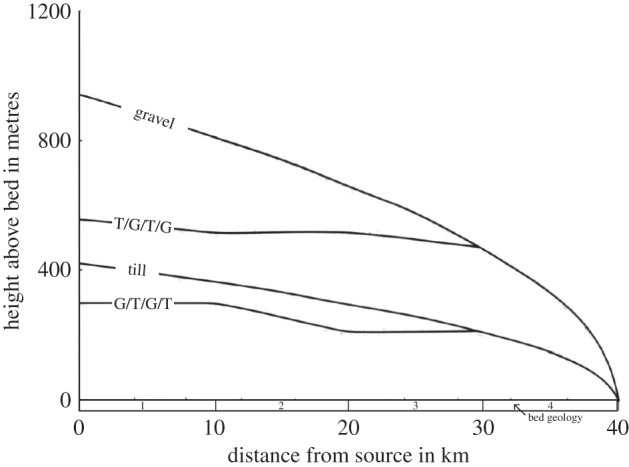
Steady-state surface profiles for an ice sheet resting on beds of gravel, till and alternating till and gravel (T/G/T/G, G/T/G/T) calculated by Boulton & Jones [144]. The distribution of basal water pressure is determined by inverting Darcy's law for computed values of the Darcy flux based on basal melt rates, and assuming a flat glacier bed. Subglacial sediment strength is determined by the Mohr–Coulomb failure criterion (4.11), with different values of cohesion and friction angle used for gravel versus till. Adapted from Boulton & Jones [144] with permission from the International Glaciological Society.
Given the timescales involved (e.g. glacial cycles), nearly all studies of groundwater circulation under ice sheets have been limited to steady state (cf. [155,158]). The subsurface is often described as a layered medium in which flow is either entirely horizontal [154,155,158] or horizontal in the more transmissive units (aquifers) and vertical in the more resistive units (aquitards) [157]. Early three-dimensional treatments were rare [156], as most model applications were confined to two-dimensional transects or paleo flowlines [157,158]. Recent work has seen increased use of three-dimensional models [151,152], though compromises are still necessary at the largest scales. In their investigation of groundwater flow beneath the North American ice sheets, Lemieux et al. [160,165] use a coarse classification of bedrock geology as one of four types (oceanic crust, orogenic belt, Canadian shield or sedimentary rocks) in order to implement their continental-scale model in HydroGeoSphere. Defining the subsurface hydrostratigraphy (thickness and properties of each hydrogeologic unit) is the only place that data figure prominently in most studies (cf. [158]). Well logs, borehole geophysical logs and outcrop studies are all relevant sources of information. Piotrowski [156] derived heterogeneous distributions of conductivity and thickness for each layer in his model based on geostatistical interpolation of such field data.
In problems examining the interplay between ice sheets and groundwater, the ice sheet is generally treated as an inert source of overburden and recharge (cf. [159]). Although most studies acknowledge the influence of ice-sheet loading on subsurface hydrogeological properties such as porosity and permeability, little account is generally taken of these effects (see [164]). Ice overburden has been used to establish Dirichlet boundary conditions (prescribed hydraulic head) in the top-most model layer [156], whereas prescribed infiltration/recharge rates are usually equated to basal melt rates of the ice sheet. In some cases, iceflow model output is used to generate temporal snapshots of basal melt rate [150,154,155,157], whereas other models simply assume a constant and uniform value (e.g. 6 mm yr−1, [158,161]). Unless the model domain extends to a hydraulic divide, some upstream boundary condition is required and often takes the form of a prescribed flux (Neumann condition). Most models assume temperate basal conditions, though the potential significance of permafrost, particularly near the ice-sheet margin and beyond, is acknowledged [157] and has been explored through prescribed model boundary conditions [152] as well as coupled modelling of ice-sheet–permafrost dynamics [159,160]).
While surface water is discussed as a potential source term in some of these studies, it was not explicitly included in ice-sheet drainage models until the work of Arnold & Sharp [58] (see §6). A surface-to-bed hydraulic connection is generally assumed to transmit water in sufficiently large quantities that some efficient drainage system at the ice–bed interface would be required for its evacuation. Most of the studies cited above conclude that subsurface aquifers are insufficient to evacuate even the basal melt generated by an ice sheet (cf. [155]), and that some interfacial drainage system is required. This excess water is dispatched through various means, from removing it instantaneously [155], to introducing a laminar film (less than 10 mm thick) at the ice–bed interface [158], to assuming Röthlisberger channels convey all subglacial water from the aquifer to the ice-sheet margin [54,136] (figure 4). The inadequacy of subsurface aquifer drainage led Piotrowski [156] to speculate on a system of cyclic water storage and release, and spurred the development of the next generation of models that would focus primarily on simulating drainage at the ice–bed interface.
Figure 4.

Conceptual model of drainage under ice sheets according to Shoemaker & Leung [136] with an aquifer overlain by an aquitard and possible drainage through R-channels. Adapted from Shoemaker & Leung [136] with permission from Wiley.
Two notable studies employ similar model physics, but stand out from the body of work described above in their application to modern ice masses: an investigation of drainage through South Cascade Glacier, WA, USA [49] (figure 5) and an early study of drainage beneath Ice Stream B, West Antarctica [55]. Campbell & Rasmussen [49] sought a simple means of relating surface meteorological conditions to proglacial discharge, and in so doing created one of the first spatially resolved numerical models of glacier hydrology. Using finite differences and an alternating-direction explicit method, they solved the transient groundwater flow equation in one dimension along a curvilinear coordinate axis following the glacier centreline. Infiltration of surface melt to the water table (recharge) was handled by calculating a time lag for the source term in the transient flow equation based on vertical seepage. Snow and ice were characterized by different values of the permeability coefficient, ksnow and kice, assumed homogeneous, isotropic and invariant with saturation. Favourable comparisons between modelled and measured discharge required realistic bed topography, and inclusion of the glacier-ice contribution to viscous retardation of water through the system. The results suggested the diurnal melt wave required more than one day to transit through the glacier (figure 5b).
Figure 5.

Drainage through South Cascade Glacier, USA, modelled by Campbell & Rasmussen [49] as a porous medium. (a) Polygons used to partition surface melt input to glacier aquifer. (b) Vertically integrated discharge in 103 m3 h−1 (solid lines) and change in saturated layer thickness in cm (2 h)−1 (dashed lines) modelled along the glacier centreline over the course of a day in 1961. Shaded area indicates increasing saturated layer thickness, and thus increasing water storage within the glacier system. Adapted from Campbell & Rasmussen [49] with permission from the author.
At a much larger scale, the same physics were applied to understand water pressures and fluxes beneath the centreline of Ice Stream B. Lingle & Brown [55] envisaged the subglacial drainage system as a single-layer porous medium of variable thickness and homogeneous isotropic hydraulic conductivity. The flowline distribution of basal effective pressure was first estimated by inverting the sliding law of Budd et al. [166], , with bed smoothness parameter c, effective pressure N=pi−pw the difference between ice and water pressures, basal shear stress τb and m=1. Sliding speed vb was calculated as the difference between the balance velocity and the deformational velocity estimated using the shallow-ice approximation. Darcy's law was then used to compute hydraulic conductivity K for a steady water flux determined from calculated sources and sinks. Profiles of bed smoothness c(x) and aquifer thickness T(x) were then iteratively estimated using additional constraints, including a requirement that pressure gradients be sufficient to drive water out of a bedrock overdeepening. Basal water pressures were determined to be in excess of 90% of flotation along the flowline, similar to the water pressures measured under the surging Variegated Glacier [45]. This led Lingle & Brown [55] to speculate that ice streams may be the manifestation of surging in ice sheets. The optimal value of hydraulic conductivity K=0.0346 m s−1 was close to the textbook value for gravel rather than till, prompting the authors to question previous interpretations of the material beneath Ice Stream B. Subsequent studies firmly established the fine-grained nature of this sediment [167], highlighting the difficulty in making direct geologic inferences from model parameters; K, in particular, is often better interpreted as an effective conductivity of the sampled drainage system, rather than a material property.
6. Next-generation glaciological models
Drainage model development through the 1990s and into the 2000s was largely motivated by a desire to more explicitly incorporate the influence of basal hydrology on ice dynamics via sliding. Most models of this generation are two-dimensional plan-view models employing a single element type to describe the morphology of the drainage system, e.g. a macroporous medium [61,62], a Weertman-type water film [57,59,63,81] or Röthlisberger channels [60] (table 2). A notable exception is the two-dimensional model of Arnold & Sharp [168] which combines descriptions of cavity- and channel-based drainage on a cell-by-cell basis, becoming the first plan-view model to incorporate multiple drainage elements.
Table 2.
Selected models, 1987–2002. Model dimension ‘2.5’ indicates two-dimensional in x–y and some representation of vertical transport.
| references | model dimension | steady-state versus transient | drainage morphology | effective pressure | water sources | coupling to dynamics | application |
|---|---|---|---|---|---|---|---|
| Budd & Jenssen [57] | two (x–y) | SS | laminar film | N=0 | modelled basal melt | yes | Ross Ice Shelf Basin, West Antarctica |
| Arnold & Sharp [58,168] | one (x), 1992; two (x–y), 2002 | SS | cavities or R-channels | equations (6.8) and (6.9) | modelled basal melt, surface melt | yes | Weichselian Scandinavian ice sheet |
| Alley [59] | one (y) | T | laminar film | equation (6.4) | — | yes | idealized mountain glacier |
| Arnold et al.[60] | 2.5 | T | R-channel network | N=0 for flow routing, channel pressures solved | modelled moulin input | no | Haut Glacier d'Arolla, Switzerland |
| Flowers & Clarke [61,62] | 2.5 | T | macroporous sheet | equation (6.14) | modelled basal melt, englacial/groundwater exchange | no | Trapridge Glacier, Canada |
| Johnson & Fastook [63] | two (x–y) | T | laminar/turbulent film | equation (6.4) | modelled basal melt | yes | Northern Hemisphere ice sheets |
(a). Ice-sheet hydrology
With the exception of two models developed for alpine glaciers [60,62], most were developed to inform ice-sheet boundary conditions, and make use of a water film [35] to describe subglacial water flow and its relationship to sliding [57,59,63,81] (figures 6 and 7). The description of film thickness d and velocity u generally assume laminar flow and follow [35]
| 6.1 |
and
| 6.2 |
with water viscosity μ, film discharge Q and fluid potential gradient ∇ϕ [57] (figure 6a). The possibility of turbulent flow was noted by Alley [59], and included by Johnson & Fastook [63] for film thicknesses d>10 cm. Instead of (6.2), they write
| 6.3 |
with Manning roughness η, hydraulic radius RH, p=2 and q=1 for laminar flow and and for turbulent flow. For the film-based models, sliding is often directly related to film thickness, rather than effective pressure. An inverse relationship between effective pressure and film thickness of the form [75]
| 6.4 |
is used to motivate sliding laws
| 6.5 |
with c=2 and r=1 [59] or r=0.5−1 [63]. An empirical approach is taken by LeBrocq et al. [81] in correlating modelled film thickness d to an inferred sliding parameter B in ub=Bτb; in this case, B is taken to be a hyperbolic tangent function of film thickness. A similar suggestion to make the sliding-law coefficient a function of film thickness was made by Budd & Jenssen [57]. Although sliding is directly related to film thickness in these approaches, effective pressure (or equivalently, water pressure) is still required to compute ∇ϕ for flow routing and film thickness and velocity. Water pressure equal to ice overburden (N=0) is typically assumed for ice sheets [57,63,81].
Figure 6.

Modelled water film thicknesses beneath the Ross Sea ice streams, Antarctica. (a) Film thicknesses contoured in millimetres by Budd & Jenssen [57]. Figure has been rotated for comparison with (b), which covers a similar domain. Adapted from Budd & Jenssen [57] with permission from Springer. (b) Film thicknesses in millimetres (colours) from LeBrocq et al. [81]. Adapted from Le Brocq et al. [81] with permission from the International Glaciological Society.
Figure 7.

Influence of basal hydrology on glacial-cycle simulations of the Northern Hemisphere ice sheets. (a) Volume of the Northern Hemisphere ice sheets modelled by Johnson & Fastook [63] with no sliding (fine solid line), sliding related to water film thickness (bold solid line) and sliding related to temperate basal conditions (dashed line). Adapted from Johnson & Fastook [63] with permission from Elsevier. (b) Ice extent along a transect through the Scandinavian ice sheet modelled by Arnold & Sharp [58] with (model 2) and without (model 1) dynamic subglacial hydrology at glacial maximum (top panel) and 3000 years after glacial maximum (bottom panel). Adapted from Arnold & Sharp [58] with permission from Wiley.
The film-based models applied to West Antarctica produce greater film thicknesses and velocities under fast-flowing regions, with maximum thicknesses on the order of approximately 5–15 mm beneath the Ross Sea ice streams [57,81] (figure 6). In Johnson & Fastook's [63] glacial-cycle simulations of the Northern Hemisphere ice sheets, the dependence of sliding on film thickness produces an ice volume record intermediate between a no-sliding case and a case with sliding related only to temperate basal conditions (figure 7a). Both sliding laws produce a lower profile ice sheet than the no-sliding case, whereas sliding-law dependence on film thickness introduces spatial structure in the flow regime thought to be consistent with evidence for paleo-ice-streams [63].
Although similar in its aims, the model of Arnold & Sharp [58,168] (figure 7b) attempts to represent efficient and inefficient drainage beneath the Scandinavian ice sheet, as well as allow for surface water as a source to the basal drainage system. The latter is computed and routed over the ice-sheet surface, whereupon it is injected directly to the bed if a prescribed threshold discharge Qcrit is reached and the bed is temperate. This threshold approach acknowledges that a critical water discharge is required to initiate and maintain a surface-to-bed connection through cold thick ice, a process that would not be well established until later [169,13]. Whether the basal drainage system is cavity- or channel-dominated is determined by the value of a flow stability parameter Λ relative to a critical value Λc [132]:
| 6.6 |
and
| 6.7 |
with a the amplitude of a representative bedrock bump and l its wavelength, A Glen's flow-law coefficient, N the effective pressure, n= Glen's flow-law exponent, the channel cross section as a function of roughness parameter fR, discharge QR and fluid potential ϕ, A* the total cross-sectional cavity area and μ a power function for self-similar bedrock [132]. In cells where Λ<Λc, channels are deemed stable and assumed to operate to the exclusion of cavities with one channel segment per 40 km gridcell. Grid-scale effective pressure is then calculated accordingly for cavities Nc or channels NR as
| 6.8 |
and
| 6.9 |
with rc a bed shadowing function [130], A and n Glen's flow-law parameters, L the latent heat of fusion, ϕ the fluid potential, discharges Qc and QR, cross-sectional areas Sc and SR and the number of flowpaths per glacier width nc. Water is routed down the fluid potential gradient ∇ϕ with pw=pi assumed. The above calculations yield mean basal water pressures of 60–80% of overburden in channel-dominated cells and 85–95% of overburden in cavity-dominated cells. As in Johnson & Fastook [63], the merits of incorporating hydrology into an ice-sheet model include spatially discriminated areas of fast flow; however, in this case, surface water and its prescribed threshold for reaching the bed, Qcrit, play a role in the manifestation and nature of these features.
(b). Glacier hydrology
Shorter timescales and smaller spatial scales, combined with access to different observables, led to alternative modelling approaches for glaciers in which the influence of surface melt is an important consideration. The seasonal drainage cycle of Haut Glacier d'Arolla, Switzerland, was simulated by Arnold et al. [60] using a network of Röthlisberger channels fed by surface water injected through moulins (figure 8a). This study stands out for its serious attempt to model surface water production and routing, in addition to englacial/subglacial water flow. It is also one of few studies where model validation is attempted, in this case through comparison of modelled and measured proglacial discharge (figure 8b), borehole water pressure and water flow velocities. A surface energy-balance scheme is used to model melt at 20 m grid scales, with vertical percolation and saturated horizontal flow accounted for within snow-covered grid cells. Water is then routed over the glacier surface to the appropriate moulin according to a topographic catchment structure, while accounting for transit time through both snow-covered and snow-free areas along the flowpath. An input hydrograph is thus derived for each mapped moulin.
Figure 8.

Drainage model of Arnold et al. [60] developed for Haut Glacier d'Arolla, Switzerland. (a) Subglacial R-channel network and moulin locations. (b) Modelled and measured proglacial discharge from Haut Glacier d'Arolla, 1993, for a simulation with a fixed drainage structure but variable channel size. Adapted from Arnold et al. [60] with permission from Wiley.
Within EXTRAN (US Environmental Protection Agency storm water management software) the Saint Venant equations are used to model water flow through the system, comprising vertical moulins and bed-parallel subglacial channels, with additional relationships describing the melt opening and creep closure of individual R-channel segments. Channel roughnesses are prescribed, but assumed to decrease with channel area. The architecture of the subglacial drainage network (figure 8a) is predefined using an upstream-area flow-routing algorithm based on subglacial fluid potential with the assumption pw=pi. Arnold et al. [60] experimented with fixed versus variable channel geometry, as well as attempting to introduce a distributed drainage system above the transient snow line by modelling flow through a bundle of tiny conduits or one broad and low conduit. Although constrained by the prescribed drainage-system structure and limited capacity for drainage system evolution, this study achieved a respectable match between modelled and measured glacier discharge (figure 8b) with a physically based treatment of englacial/subglacial drainage. A similar approach has been taken to model subglacial water routing in a catchment of western Greenland [170,171].
A simple yet comprehensive approach to modelling drainage through polythermal Trapridge Glacier was the goal of Flowers & Clarke [61,62,172] in constructing a multi-layer model representing surface, englacial, subglacial and groundwater drainage systems (figure 9). Two-dimensional plan-view water flow is modelled in each layer, with vertical exchange between adjacent layers (figure 9a inset) parametrized in terms of fluid potential gradients and solved simultaneously as coupling terms ψ in the respective continuity equations
| 6.10 |
| 6.11 |
| 6.12 |
| 6.13 |
with hr, he, hs and ha the areally averaged water volumes in the respective layers, M and bs the surface and basal source terms, qr, qe, qs and qa the horizontal fluxes in each layer, ψ the exchange terms between adjacent layers and ρa the groundwater density. Horizontal fluxes adopt the form of Darcy's law, with the interpretation and form of the hydraulic conductivity K varying by layer; K is written as for a fractured medium to describe the englacial drainage system, whereas it varies with hs in the subglacial system to emulate variable efficiency. To close the equations without assuming pw=pi, a relationship of the form
| 6.14 |
is adopted [61,62], with critical sheet thickness hc corresponding to flotation water pressures and derived from Trapridge Glacier borehole drilling data. This ad hoc relationship requires prescription of hc, but produces an inverse relationship between sheet thickness and effective pressure as in (6.4) and allows glaciological water pressures to be achieved for plausible macroporous sheet thicknesses of decimetres. Borehole water pressure data were used to tune model parameters unconstrained by other field observations (figure 9b), and the model was used to demonstrate qualitative characteristics of the seasonal cycle of glacier hydrology [62] as well as the response to a hydromechanical event documented by a variety of subglacial sensors [172]. A similar model, stripped of its surface and englacial layers, was applied to the larger scales of two Icelandic icecaps [173–176].
Figure 9.

Drainage model of Flowers & Clarke [172] developed for Trapridge Glacier, Yukon, Canada. (a) Conceptual model illustrating (1) supraglacial, (2) englacial, (3) subglacial and (4) groundwater drainage. Reprinted from Flowers & Clarke [172] with permission from the International Glaciological Society. (b) Modelled subglacial water pressures (dashed line) compared with mean measured values from 16 pressure transducers (solid line) within a single model gridcell [62]. Adapted from Flowers & Clarke [62] with permission from Wiley.
The strong observational basis for morphological transitions in the subglacial drainage system [93] motivated Arnold et al. [60] and Flowers & Clarke [61] to emulate aspects of these transitions without the need to alter model physics. Channels of different diametres and aspect ratios were used to mimic distributed (inefficient) drainage in the channel-based model of Arnold et al. [60], while a rapid increase in system transmissivity was used to mimic an abrupt increase in drainage efficiency in the macroporous model of Flowers & Clarke [61]. Neither approach was particularly successful. While some of the earlier models had already attempted to include fast (channelized) and slow (distributed) drainage [54], the next phase of model development would see increased attention paid to more properly representing the physics of fast and slow drainage elements.
7. Multi-element models
Longstanding observational studies of mountain glaciers (for review, see [23,24,146] for review), and more recent studies from the margins of the Greenland ice sheet [11,177], point to profound spatial and temporal variations in subglacial drainage-system morphology, itself defined by the presence and interaction of various drainage elements. Clarke [178] devised one of the first multi-element drainage models using hydraulic analogues to electrical circuits (figure 10). Circuit elements representing water sources and sinks, flow resistors, water storage and system switches are combined in series and parallel to produce hydraulic head responses reminiscent of borehole water-pressure records. Multi-element lumped models have been used to explain the results of dye-tracing experiments on alpine glaciers [179,180] and to interpret short-term flow variability of land-terminating Greenland outlet glaciers [181]. Subsequent development has focused on spatially resolved models, at the expense of this broad range and diversity of drainage elements (table 3).
Figure 10.

Clarke's [178] lumped model of glacier drainage based on hydraulic analogues to electrical circuits. (a) Symbols represent input discharge (Q0, Qp, Qm), hydraulic resistors characteristic of winter (R1W, R2W) and summer (R1S, R2S) drainage, switches (SW-1, SW-2), closed elastic storage (V2) and Darcian leakage (D1). (b) Hydraulic head response (solid lines) at nodes 1 and 2 to input discharge Q0 (dashed line) with activation of switches SW-1 and SW-2 at times t1 and t2. Adapted from Clarke [178] with permission from Wiley.
Table 3.
Selected multi-element drainage models, 1992–2014. *Insofar as sliding is used to determine whether drainage is cavity- versus channel-dominated.
| references | model dimension | slow-system morphology | fast-system morphology | drainage a function of sliding? | coupled to iceflow model? | application |
|---|---|---|---|---|---|---|
| Clarke [178] | lumped | various | various | no | no | generalized glacier system |
| Arnold & Sharp [58] | one | cavities | R-channels | yes* | yes | Scandinavian ice-sheet |
| Flowers et al.[64] | one | laminar/turbulent sheet | R-channels | no | no | Skeidarárjökull, Iceland |
| Kessler & Anderson [65] | one | cavities | R-channels | yes | no | idealized glacier |
| Flowers [182] | one | macroporous sheet | R-channels | no | no | idealized glacier |
| Hewitt & Fowler [66] | one | cavities | R-channels | yes | no | idealized glacier |
| Colgan et al.[183,184] | one | englacial storage | R-channels | no | yes | Sermeq Avannarleq, Greenland |
| Pimentel & Flowers [185] | one | macroporous sheet | R-channels | no | yes | idealized outlet glaciers |
| Hewitt et al.[121] | one | cavities | R-channels | yes | no | idealized outlet glacier |
| Kingslake & Ng [67] | one | cavities | R-channels | yes | no | idealized mountain glacier |
| Schoof et al.[186] | one | cavities | R-channels | yes | no | idealized mountain glacier |
| Arnold & Sharp [168] | two | cavities | R-channels (1 per cell) | yes* | yes | Scandinavian ice-sheet |
| Schoof [70] | two | cavities | R-channels (two-dimensional) | yes | no | idealized ice-sheet margin |
| Hewitt [68] | two | cavities | R-channels (one-dimensional) | yes | no | idealized ice-sheet margin |
| Hewitt [71] | two | cavities | R-channels (two-dimensional) | yes | yes | idealized ice-sheet margin |
| Werder et al.[72] | two | cavities | R-channels (two-dimensional) | yes | no | idealized ice-sheet margin, Gornergletscher |
| de Fleurian et al.[187] | two | porous medium | porous medium | no | yes | Haut Glacier d'Arolla |
| Hoffman & Price [69] | two | cavities | R-channel (one-dimensional) | yes | yes | idealized mountain glacier |
| Bougamont et al.[73] | 2.5 | till (z) | water routing scheme (x–y) | yes | yes | Russell Glacier catchment, West Greenland |
(a). One-dimensional models
One-dimensional multi-element models have proliferated in the past decade (table 3), variously motivated by studies of ice-dammed lake drainage [64,65,67,185], the seasonal evolution of glacier drainage and dynamics [65,66,183,185], the imprint of subglacial processes on discharge hydrographs [182] and oscillatory winter water pressures [186]. While the intended model applications are diverse, model demonstration is often limited to idealized settings. Nearly all models adopt the same basic elements to describe fast and slow drainage (table 3), but differ in the details of their implementation.
The assumption of a single evolving R-channel is common in one-dimensional multi-element models [67,185] and present in some form in some two-dimensional models [68,69,168]. Such an assumption can be justified for modelling a classical outburst flood [67] or drainage beneath an individual valley glacier [66] where discharge is likely to be dominated by a single channel. For a single saturated channel, conservation of ice and water mass, respectively, lead to
| 7.1 |
and
| 7.2 |
for conduit cross-sectional area S, discharge Q, flow-following coordinate s, fluid potential ϕ, water pressure pw, latent heat of fusion L, Glen's flow-law coefficient A and exponent n, γ=ρwctcp (see §4b) and source term bc. For saturated turbulent pipe flow, discharge is the product of velocity v and cross-sectional area S:
| 7.3 |
where for the common Darcy–Weisbach formulation,
| 7.4 |
with wetted perimeter Pwet, roughness fR, hydraulic radius RH and Manning roughness η′. Common model variations include (i) assuming semicircular (S=πr2/2, RH=πr/2(π+2), Pwet=r(π+2)) versus circular (S=πr2, RH=r/2, Pwet=2πr) channels, (ii) direct prescription of the Darcy–Weisbach friction factor fR rather than the Manning roughness η′, the latter approach permitting wall roughness to decrease with channel size (see [127]) and (iii) neglect of the pressure melting term γ, which reduces (or augments) the energy available for wall melting for water flow from high to low (or low to high) pressure [188].
Attempts to include more than a single channel in a one-dimensional multi-element model have either prescribed a latent channel spacing [64] (figure 11a) or a variable number of channel segments per unit width [183]. The former was inspired by the observed activation of multiple channels across a glacier margin during an outburst flood [64] and the objective of simulating broad-scale ice-sheet margins where more than one channelized outlet might be expected. It requires only a trivial modification to the water balance equation to partition source water between multiple channels, while leaving the channel evolution equation unchanged under the assumption that channels evolve identically. Subsequent work has demonstrated that the effective transmissivity of the distributed drainage system and channel spacing are related [68], so caution should be exercised in using models where these parameters are prescribed independently. Another approach [183] is predicated on the widely held notion that channel-dominated drainage systems are arborescent, with smaller more numerous branches upstream converging into fewer major channels downstream; Colgan et al. [183] prescribe an exponential decrease in channel spacing and maximum channel radius as a function of distance upstream from the terminus. Two-dimensional plan-view modelling of the drainage system suggests that valley glacier geometries can produce dendritic drainage networks [72], while ice-sheet-like geometries characterized by flatter beds and laterally uniform ice thicknesses produce quasi-regularly spaced flow-parallel channels in steady state [71].
Figure 11.

One-dimensional multi-element conceptual models of subglacial drainage. (a) Coupled flow-parallel R-channels, a macroporous sheet and groundwater aquifer in Flowers [182]. Adapted from Flowers [182] with permission from Wiley. (b) Coupled R-channel and linked cavities in Kessler & Anderson [65]. Adapted from Kessler & Anderson [65] with permission from Wiley. (c) Coupled R-channel, cavity system and ice-dammed lake in Kingslake & Ng [67]. Adapted from Kingslake & Ng [67] with permission from the International Glaciological Society.
Representation of the slow drainage system in one-dimensional multi-element models is straightforward for an effective porous medium in which some form of Darcy's law describes water flux, and drainage-system evolution is confined to the fast system [182,185]. Although a cavity system may be described as an effective porous medium at the scales relevant to drainage modelling [68], most cavity-based models include some representation of cavity-system evolution which the porous sheet models lack. Hewitt & Fowler [66] and Kingslake & Ng [67] take similar approaches in which the description of the cavity system follows the analysis of Walder [40] (see §4c) in relating cavity-system cross-sectional area Sc, discharge Qc, basal effective pressure Nc and sliding speed ub, e.g.
| 7.5 |
| 7.6 |
| 7.7 |
for constants βc, γc, c, p and q, Glen's n and basal shear stress τb [66] (figure 12a). Cavities thus open by sliding and close by creep, whereas melt opening is restricted to channels. Simplifying assumptions in this approach include the specification of a constant cavity-forming obstacle height (e.g. 0.1 m in reference [67]). In both models, coupling between hydrology and dynamics occurs through the relationship between sliding speed ub, cavity-system effective pressure Nc and cavity-system cross section Sc.
Figure 12.

Effective-pressure–discharge relationships for cavity–channel models. (a) Calculated steady-state effective pressure as a function of discharge in cavities (solid line) and channels (dashed line) from Hewitt [68]. Adapted from Hewitt [68] with permission from the International Glaciological Society. (b) Calculated steady-state effective pressure as a function of water input for cavity-like drainage (diamonds) and channel-like drainage (circles) from Schoof et al. [186]. Stable solutions are shaded solid. Adapted under the Creative Commons License.
Schoof et al. [186] exploit a unified description of cavities and channels as end-members of a conduit element, where each model node represents a single conduit that can evolve into an R-channel or cavity as dictated by hydraulic conditions [41,70]. The conduit evolution equation of Schoof et al. [186] includes, in order, terms representing melt opening, opening due to sliding and creep closure:
| 7.8 |
with conduit cross-sectional area S, positive constants c1, c2, v0 and S0, discharge Q, hydraulic potential ϕ, effective pressure N and Glen's n. This formulation allows spontaneous evolution of a distributed or channelized system (figure 12b) by retaining all sources of conduit opening and closure. Distributed englacial storage connected to the basal drainage system thus envisioned plays a key role in this model, driving intriguing oscillations (limit cycles) in basal effective pressure reminiscent of jökulhlaups. These oscillations only occur over a limited range of basal water supply (open symbols in figure 12b) [186].
Kessler & Anderson [65] similarly model a cavity system governed by melt opening, opening owing to sliding and creep closure. This system is comprised of high-tortuosity semicircular channels roughly orthogonal to ice flow and confluent with the arterial channel along the glacier centreline (figure 11b). The feeder-channels are cavity-like in that (i) sliding increases their cross sections (for two different prescribed bed-obstacle wavelengths) and (ii) the hydraulic head gradient is concentrated along a limited fraction () of the channel length taken to represent ‘orifices’ connecting numerous cavities (after [41]). This conceptual model inspired the spatially lumped cavity-system model of Bartholomaus et al. [189] applied to Kennicott Glacier, Alaska, to relate water storage to sliding speed derived from GPS records of surface motion. In the model of Kessler & Anderson [65] (and Bartholomaus et al. [189]) developed for valley glaciers, as well as that of Colgan et al. [183,184] applied to the margin of the Greenland ice sheet, englacial storage is assumed perfectly connected to the basal drainage system. The height of water within the englacial system, characterized as a macroporous medium, sets the hydraulic head at the bed. Changes in water input to the englacial system therefore directly drive changes in basal water pressure.
The unified treatment of fast- and slow drainage systems in the model of Schoof et al. [186] obviates the need for an explicit statement of water exchange between the two systems. Similarly, in treating the cavity system as tortuous channel-like tributaries, Kessler & Anderson [65] explicitly integrate the tributary contributions to discharge in the main arterial channel without invoking additional physics to describe cavity–channel water exchange. This particular approach assumes one-way flow between tributary and trunk channels. In most other one-dimensional multi-element models, water exchange is governed by pressure differences between the fast and slow systems under the assumption that both reside at the same elevation. In [64,182,185], this takes the form
| 7.9 |
with a valve represented by χs:c=[0,1], effective hydraulic conductivity and water depth at the sheet–conduit interface Ks:c and hs:c, latent conduit spacing d and sheet- and channel water pressures ps and pc. In Hewitt & Fowler [66] and Kingslake & Ng [67], exchange is similarly written
| 7.10 |
for constant k and effective pressures in the R-channel and cavity systems NR and Nc. In (7.9) and (7.10), water exchange between fast and slow drainage systems forms part of the solution and can take place in either direction.
With appropriate physics employed to describe the evolving morphology of the drainage system, multi-element models are generally better than their predecessors in simulating phenomena such as seasonal transitions (figure 13). Models coupled to sliding further allow simulation of seasonally accelerated iceflow associated with melt input (e.g. figure 14a) [65,66,184,185], perturbations to iceflow associated with flooding (e.g. figure 14b) [67,185] and hydrologically sensitive rates of deglaciation (e.g. figure 7) [58].
Figure 13.

Seasonal transition in drainage system morphology simulated with the simple one-dimensional sheet–conduit model of Flowers [182] (figure 11a). Each panel shows a variable (colour) plotted as a function of position downglacier (horizontal) and day number during the melt season (vertical). (a) Sheet–conduit water exchange. Positive values indicate water flow from the distributed sheet to the developing conduit system. (b) Conduit cross-sectional area, reflecting conduit growth and decay through the melt season. (c) Sheet discharge, peaking early in the melt season. (d) Conduit discharge, peaking late in the melt season. Adapted from Flowers [182] with permission from Wiley.
Figure 14.

Results of one-dimensional multi-element models coupled to sliding. (a) ‘Spring event’ simulated by Kessler & Anderson [65] with conceptual model in figure 11b. Upglacier incision of arterial channel (second panel), modelled sliding speed (third panel) for locations colour-coded in top panel and input (dashed) versus output (solid) discharge (bottom panel) highlighting times of increasing (shaded) and decreasing (unshaded) water storage. Adapted from Kessler & Anderson [65] with permission from Wiley. (b) Outburst flood simulation by Kingslake & Ng [67] with conceptual model in figure 11c. Lake level hL and discharge into conduit QR (upper left), modelled sliding speed at four locations along the glacier (lower left), cavity–channel water exchange as a function of distance downglacier and time (right) with positive values indicating water flow from the cavity system to the channel. Adapted from Kingslake & Ng [67] with permission from the International Glaciological Society.
While some of the one-dimensional models in table 3 are coupled to one- or two-dimensional iceflow models [58,184,185], the interaction between hydrology and dynamics is commonly demonstrated through sliding alone, for example, using the power-law in (7.7) [66,67]. Arnold & Sharp [58] adopt the sliding relation of McInnes & Budd [190],
| 7.11 |
with constants k1 and k2, and effective pressure N calculated according to drainage system structure following (6.8) or (6.9). Kessler & Anderson [65] introduce a sliding threshold pt, such that non-steady sliding occurs only above pt according to
| 7.12 |
with constant B and basal shear stress τb (see also [191]). Pimentel & Flowers [185] employ a Coulomb-friction law to describe sliding [192,193],
| 7.13 |
where C is a constant and Λ depends primarily on the geometry of bed obstacles involved in cavitation. Colgan et al. [184] use an empirical sliding law in the spirit of Bartholomaus et al. [189]:
| 7.14 |
where ub0 is a steady background sliding speed, nc is the number of channel segments per unit width of the glacier, k(x) is a tuning parameter, x is the longitudinal coordinate, m is set to 3 and ∂he/∂t is the rate of change of hydraulic head in the englacial aquifer (storage). Sliding does not exceed ub0 for |∂he/∂t|<0.25 m d−1.
(b). Two-dimensional models
Recent advances in the numerical representation of two-dimensional multi-element drainage systems have produced results of unprecedented realism [70–72], particularly in the simulation of spontaneous channel networks (figures 15 and 16). The first of these models is identical to that of Schoof et al. [186], but with each edge of a two-dimensional numerical mesh fitted with an individual conduit element. Each element can evolve into a cavity or an R-channel according to the balance of opening and closure processes (equation (7.8)), thus forming a network of interconnected channels even in the presence of uniformly distributed water input (figure 15).
Figure 15.

Two-dimensional steady-state drainage network simulated by Schoof [70] over an inclined glacier bed of 10×20 km with uniform water input. (a) Conduit cross-sectional area S highlighting the major channels. (b) Contours of effective pressure N showing increased N in the vicinity of channels. Adapted from Schoof [70] with permission from Macmillan Publishers.
Figure 16.

Simulations of subglacial drainage with two-dimensional models comprising cavity systems coupled to a network of spontaneously evolving R-channels. (a) Seasonal evolution of basal drainage (left column) and surface flow speed (right column) for an idealized outlet glacier simulated by Hewitt [71]. Blue shading indicates subglacial discharge and red contours subglacial effective pressure (left), whereas grey dots (left and right) show moulin locations through which surface melt is funnelled to the bed. Adapted from Hewitt [71] with permission from Elsevier. (b) Subglacial channel network after 200 model days for Gornergletscher, Switzerland, simulated by Werder et al. [72]. Channels are shown as blue lines with thicknesses coded by discharge (see legend). Basal effective pressure is shown in colour. Moulins are randomly distributed, with dot size proportional to melt input. Ice and water flow are generally from right to left. Adapted from Werder et al. [72] with permission from Wiley.
The models of Hewitt [71] and Werder et al. [72] (figure 16) (see also [121,194]) retain the treatment of the incipient channel system as defined along the edges of the numerical mesh, but incorporate a continuum description of distributed drainage whereby a system of cavities is defined within the mesh elements [68]. This description permits more than one cavity per gridcell, with cavities assumed identical in nature and the distributed system thus described as a ‘sheet’ with an effective transmissivity khα and
| 7.15 |
where α=3 and β=2 for laminar flow in Hewitt [68,71] and and for turbulent flow in Werder et al. [72]. Constant k is prescribed directly by Werder et al. [72], but cast as k=k0/ηw with permeability k0 and fluid viscosity ηw in Hewitt [68] and k=K/ρwg for hydraulic conductivity K in Hewitt [71]. The evolution of sheet thickness h takes the form of (3.5) and is related to the characteristic height of cavity-forming bed obstacles hr and their spacing lr as
| 7.16 |
with Glen's n and the ice flow-law coefficient including a multiplier that depends on cavity geometry. Englacial water storage, either in moulins or in some distributed reservoir, is included in references [71,72] as a function of sheet water pressure pw and a prescribed englacial void ratio ev: he=evpw/ρwg. This storage term damps transients in the drainage system, including diurnal oscillations, but does not affect steady-state solutions. The continuity equation for coupled water flow in the sheet and channel system, including englacial storage, can then be written [71]
| 7.17 |
with q as in (7.15), S the cross-sectional area of a conduit segment and s its flow-following coordinate here constrained to lie along the mesh edges, Q the conduit discharge, V the volumetric storage of water in moulins, m the basal melt rate, M the melt rate owing to viscous dissipation of heat in the conduits, R the source term to the moulins and δ(xm) and δ(xc) delta functions defining specified point locations of moulins and line locations of conduits, respectively.
This continuum description of the cavity system was first implemented by Hewitt [68] with channels treated as one-dimensional flow-parallel elements, and later implemented in a two-dimensional finite-difference framework and coupled to iceflow [71] (figure 16a). Finite-element descriptions of the cavity system and the coupled cavity–channel system were given in one-dimension by Schoof et al. [194] and Hewitt et al. [121], respectively, and then in two-dimensions by Werder et al. [72] (figure 16b). Although the description of the continuum cavity system may resemble an effective porous medium, it differs from the macroporous sheet in [182,185] in that (i) flow is generally assumed turbulent, rather than laminar (equation (7.15)), (ii) the sheet opens by sliding as in most of the one-dimensional cavity-based models (7.16) and (iii) water pressures are assumed identical between adjacent sheet and channel elements. The latter obviates the need for an explicit representation of water exchange as in [66,67,182] (e.g. equations (7.9) and (7.10)). Rather, water exchange is accomplished in such a way that sheet and channel pressures match at their boundaries. With this constraint, and the additional governing equation for h (7.16), an explicit relationship between sheet thickness h and pressure pw need not be defined (cf. [64,182,185]).
In separating channel elements from the cavity system, the models of Hewitt [71] and Werder et al. [72] also differ from those of Schoof et al. [70,186] and Kessler & Anderson [65] by applying all energy for melt opening to the channel elements, rather than the cavities. This small conceit is necessary and requires a parameter to describe the width over which channels collect melt energy from the cavity system [71,72]. These models yield robust simulations of classical drainage system behaviour on both synthetic [71] (figure 16a) and real topography [72] (figure 16b). The models have also demonstrated important consequences of the physics governing drainage, such as (i) the tendency for laterally homogeneous glacier geometry to produce non-arborescent flow-parallel channels in steady state, (ii) the existence of ‘blind’ channels that terminate before reaching the glacier margin and lead to convex, rather than concave, perturbations to the neighbouring hydraulic potential and (iii) the sensitivity of drainage structure in the presence of significant bed slopes to the often-neglected pressure-melting term in the conduit evolution equation (7.2) [72,188].
Two other two-dimensional approaches to modelling multi-element drainage have recently been taken. Hoffman & Price [69] largely follow the formulation of Hewitt [68] in describing a single channel nested with a system of cavities. They do this within the framework of the Community Ice Sheet Model using finite differences. de Fleurian et al. [187] incorporate a two-layer basal drainage model in the finite-element full-Stokes model Elmer/Ice, in which Darcy's law governs laminar flow in both fast and slow drainage systems [61]. These systems are characterized by contrasting values of prescribed hydraulic transmissivity and storativity. Both approaches [69,187] require somewhat arbitrary activation of the fast drainage system, precluding internally driven two-way morphological transitions (e.g. slow-to-fast and fast-to-slow). Hoffman & Price [69] define a dissipation factor Df as the ratio of cavity opening due to melt versus sliding:
| 7.18 |
with water flux q, potential gradient ∇ϕ, sliding speed ub, sheet thickness h, bed obstacle height hr and wavelength lr. Dissipation q⋅∇ϕ/ρiL is not applied to the cavity system [71,72], but rather computed for the purpose of calculating Df. When Df≥1, a single channel is activated within the domain and then evolves based on water exchange with the cavity system; exchange is governed by a lateral Darcy-like flux (as in references [64,66,67]). In the model of de Fleurian et al. [187], the efficient drainage layer is activated where and when required to maintain effective pressure N≥0 in the inefficient system (not unlike [158]). The efficient drainage system grows spatially by similar rules until it reaches an outlet, after which water exchange between the two systems is governed by a Darcy discharge that depends on a ‘leakage length scale’. Once activated, the efficient layer becomes permanent but water exchange can still occur in either direction. Both the above models couple hydrology and dynamics through some form of the Coulomb-friction law (7.13), and illustrate the glacier response to meltwater input. Hoffman & Price [69] specifically investigate the importance of two-way coupling between hydrology and dynamics, demonstrating the significant braking potential of cavity opening by sliding when two-way coupling is present (figure 17).
Figure 17.
Sliding response to basal water input for cavity-only (solid lines) and cavity–channel (dashed lines) drainage systems, with one-way (black lines) and two-way (red lines) coupling to dynamics in Hoffman & Price [69]. Water input is turned on at time zero, causing an increase in sliding that peaks and decays even in cavity-only simulations (solid black and red lines) owing to increased melt opening of cavities. Channel formation (dashed lines) causes a pronounced decrease in sliding below the initial value. The difference between red and black lines illustrates a significant negative feedback on sliding with two-way coupling (cavity opening rates increase with sliding), including delayed channel formation. Adapted from Hoffman & Price [69] with permission from Wiley.
In a departure from most other multi-element models, Bougamont et al. [73] combine a plan-view subglacial water routing scheme [85] with a sediment model that allows vertical transport of water into and out of the till [195]. A fast drainage system is assumed to exist at the ice–bed interface as needed, but not explicitly modelled. Surface and basal meltwater contribute to a subglacial water film of the form (6.1) which partially governs the vertical flux of water into a 5 m-thick till layer. ‘Excess pore pressure’ (pressure above hydrostatic) reduces sediment shear strength τ* through the Mohr–Coulomb failure criterion (4.11) with cohesion set to zero such that
| 7.19 |
and
| 7.20 |
where e is void ratio, a function of porosity n=e/(1+e), e0 is the reference void ratio at effective stress N0, ψ is the friction angle and C is the compression index. The novelty of this study is the application of a soft-bed hydrology model to Greenland, where although there is evidence for subglacial sediments [196], most models have assumed an impermeable bed. Bougamont et al. [73] suggest that soft-bed dynamics, namely the watering (weakening) and dewatering (strengthening) of till in response to vertical hydraulic gradients, provide an alternative explanation for the seasonal velocity cycle observed in western Greenland.
8. Models of Antarctic basal hydrology
Since the work of Budd & Jenssen [57], little large-scale hydrological modelling has been undertaken for the Antarctic ice sheet (cf. [81]). What has been done at the basin to continental scale has largely comprised implementation of algorithms for water routing [197,198] based on steady-state hydraulic potential structure computed from ice-sheet digital elevation models and estimates of basal melt or freezing [85,199–202]. While most large-scale ice-sheet models include sliding [203,204], few have attempted to relate sliding to hydrological variables (cf. [205,206]). Much of the effort has instead focused on modelling processes under ice streams [75], and since 2006, subglacial floods [2].
Attempts to understand Antarctic subglacial floods [2], including quantifying variables such as conduit size and peak discharge, have borrowed heavily from the theoretical principles of Röthlisberger [43], Nye [117] (e.g. [2,83,84]) and Walder & Fowler [138] (e.g. [207]). This problem is made difficult by validation data being limited to ice-surface elevation changes associated with lake filling and draining. To understand the role of lakes within the broader drainage system, spatially distributed modelling studies [85,199,208] have relied upon various implementations of steady-state flow routing algorithms [209].
While subglacial water has been included in coupled ice–till flow models to relate melt rates, void ratios, and till deformation [76,77,210–213], few models have attended to representing the drainage system itself (cf. [78,214]). Models that do treat hydrology have been developed for the Siple Coast ice streams, which are underlain by thick saturated sediments and lack strong topographic controls. Conceptual models thus employ water sheets [74] or porous flow [55], with localized drainage structures (e.g. canals) [139] only recently introduced [214].
Much of the recent work can be traced back to Alley [75] who considered water flow over the unconsolidated bed of ice stream B (now Whillans Ice Stream). Alley describes end-member models in which all water is conveyed in subglacial till (groundwater flow) versus all water being conveyed at the ice–bed interface. Channelized drainage is dismissed based on the relative efficacy of inward creep of sediment in an incipient channel, compared with sediment erosion by water flow. Subsequent investigations of till creep in the vicinity of canals concluded that (i) its lateral extent would be limited for thin till [137], (ii) creep rates depend critically on till permeability [140] and (iii) the role of creep is partially determined by the sediment budget along the canal [139,142]. For effective pressures characteristic of ice streams, Alley [75] argues that water would flow in a film several millimetres thick over a saturated till bed [74].
Sheet-like drainage under ice streams has been adopted by Kyrke-Smith et al. [78] in a two-dimensional plan-view model coupled to ice flow that exhibits spontaneous development of ice streams. A Weertman-like sheet overlies a saturated low-permeability till, and becomes unstable when it decouples from its supporting clasts [114] (figure 18a). This instability, which occurs at a critical water depth related to clast size, is responsible for the initiation of streaming (figure 18b). Streaming perpetuates through the deflection of water toward the ice streams and the enhanced production of basal melt due to steepening of the surface slope in the onset region. Analysis of the hydrologically coupled model suggests the possibility of a triple-valued relationship between ice thickness and velocity that depends on the critical sheet depth. Model simplifications include the assumption of temperate bed conditions and partial treatment of thermal processes (such that energy is not conserved), the use of idealized domain geometry, omission of sediment transport (including by till deformation) and a limit on water depth to prevent N=0. When sediment transport is added to the model [79], wide and shallow stable waterways develop through the combined effects of fluvial transport and shearing and squeezing of the saturated till.
Figure 18.

Conceptual models for drainage over unconsolidated beds and models of Antarctic ice streams. (a) Clast-supported water sheet of Creyts & Schoof [114]. Adapted from Creyts & Schoof [114] with permission from Wiley. (b) Simulation of sliding velocity (top panel) and subglacial water depth (bottom panel) by Kyrke-Smith et al. [78] after 360 model years during which ice streams form within the domain. Adapted under the Creative Commons License. (c) Conceptual model for drainage under Kamb Ice Stream according to van der Wel et al. [214] with broad shallow conduits incised in ice and till. Adapted from van der Wel et al. [214] with permission from Wiley.
The role of hydrology in generating ice-stream-like flow oscillations is investigated by van der Wel et al. [214] using a coupled model of ice, water and till in which subglacial canals are present (after Ng [142]; figure 18c). A Coulomb plastic rheology is assumed for the undrained 4 m-thick till layer of reference porosity 0.4 intended to emulate the conditions beneath Kamb Ice Stream (as in reference [76]). Effective pressure N is controlled by the till void ratio e according to (7.20) with e0=0.6 and C=0.25, while the Mohr–Coloumb criterion in (4.11) with cohesion c0=1 kPa sets the sediment shear strength. Ice and till thicknesses, water fluxes and thermal processes together control the void ratio e. A fixed number of flow-parallel canals are prescribed, but activated only when till porosity reaches its prescribed maximum value. Flow in the canals can be either laminar or turbulent based on the Darcy–Weisbach flux relation. Effective pressure in the canals is given by
| 8.1 |
where Qc is canal discharge and Kn is a complicated function that depends on the square root of the sediment flux. Water pressure in the canals can then be calculated from (8.1) and the ice-overburden pressure. Water fluxes into the canals are prescribed at the upstream boundary to represent inflow from subglacial lakes. The presence of canals that reach the grounding line generally increases the ice-stream oscillation period; in simulations without extensive canal activation, the oscillation period is regulated by thermal conditions alone. The primary role of the canal system in this model is to augment porewater availability for basal melting or refreezing, thereby altering the till void ratio and basal effective pressure. Temporal modes of ice-stream variability are also identified in the spatially lumped modelling of Robel et al. [215], where both thermal and hydrological controls on till properties are considered.
9. Summary and outlook
Since the early 1970s, subglacial drainage models have progressed from groundwater models applied directly to glaciers and ice sheets, to models that now capture realistic plan-view evolution of multiple, interacting drainage components. This progress is anchored in the theoretical foundations laid in the 1960s–1980s that established the mathematical details of various drainage ‘elements’. The most sophisticated models to date still draw directly from this early work, but have overcome the challenge of incorporating fundamentally one-dimensional and subgrid-scale structures (e.g. R-channels, individual cavities) in a two-dimensional continuum framework. Models have succeeded in (i) applying the correct physics to interacting fast- and slow drainage systems, (ii) adopting a numerical framework that elegantly suits the physics of the problem, (iii) simulating drainage-system evolution, including the spontaneous development of channel networks, in response to distributed and point-sources of water and (iv) two-way coupling between glacier hydrology and dynamics. Models developed specifically for Antarctic environments consider the coupled thermal and hydrological controls on ice flow, with attempts to represent increasingly realistic basal drainage and its influence on the spatial and temporal variability of ice streaming.
In pushing the science forward on these fronts, simplifications in other areas are necessary. Many of the current models, inspired heavily by observations from Greenland, presently assume temperate conditions and prescribe water input to the bed. Antarctic models are common exceptions to this, where thermal conditions cannot be ignored and source terms are generally limited to water derived from basal melt. The most sophisticated models designed for settings in which surface melt is important, nearly unanimously use the classical and tractable descriptions of R-channels and cavities to represent fast- and slow drainage, respectively. Such models require a numerical mesh that resolves individual channel segments.
Each of these simplifications presents an opportunity for further work. Future efforts should consider whether our current conceptual models embrace the full menagerie of necessary drainage elements, and whether a more unified treatment of hard- and soft-bed hydrology is warranted. We must also grapple with how best to represent basin-scale drainage networks in continental-scale models. Finely resolved models that simulate channel network evolution could be used to train coarsely resolved models that implement a statistical description of drainage system behaviour. Such models could be applied at the whole-ice-sheet scale with a reduced computational burden, filling a niche between the most sophisticated models and the simplest but most efficient ones.
Models would ultimately benefit from internally consistent and coupled treatment of water flow from the surface to the subsurface, taking advantage of progress in modelling supraglacial [216], englacial [17,18,217,218] and groundwater drainage [80]. Any model striving for broad applicability will have to treat polythermal bed conditions [188,206,214], a complication often neglected but potentially important for both drainage and ice dynamics [219,220]. In addition to a thermal patchwork at the glacier bed, direct observations of subglacial conditions (e.g. through boreholes) consistently affirm the heterogeneity of the drainage system and the importance of ‘connected’ versus ‘unconnected’ areas [104,221,222]. Until we develop alternatives to the present continuum models, or devise a means of including the unconnected bed, our ability to simulate drainage system fragmentation, high winter water pressures and more than a small fraction of the phenomena present in borehole water pressure records will be limited.
Finally, recent model development has outstripped the pace at which the data necessary for exploiting the full capabilities of the models, let alone performing respectable calibrations, are generated. More accurate and detailed maps of glacier-bed topography [223] are needed to resolve influential features of the drainage system [12], including the effects of pressure-melting on channel network architecture [72]. Even with detailed input data, models of basal drainage will continue to suffer from a lack of direct, independent and applicable data for calibration. Borehole records are the closest we have to direct observations of the basal drainage system, yet suffer from being point-scale in nature. An ambitious observational target would be a remote method of directly measuring variables relevant to basal drainage (e.g. water pressure, water depth, effective pressure, discharge) averaged over the relevant spatial scales.
With growing interest in whole-ice-sheet models of basal hydrology, near-term developments will still require parsimonious representation of drainage-system elements while retaining the salient influence of hydrology on basal processes. While the current focus seems squarely on developing drainage models for the purpose of informing ice-sheet boundary conditions, interest in subglacial chemical, erosional and biological processes may ultimately drive renewed interest in hydrology modelling in its own right.
Acknowledgements
I have had the privilege of working with and around people who have made outstanding contributions to our understanding of subglacial drainage modelling. For conversations old and new, I thank Garry Clarke, Helgi Björnsson, Tim Creyts, Christian Schoof, Ian Hewitt and Mauro Werder. I am grateful for the invitation to write this review, and to Richard Hindmarsh and Frank Pattyn for an opportunity to speak on this subject at the IGS-Chamonix Symposium in May 2014. Jean-Michel Lemieux pointed me to new literature on paleo-ice-sheet hydrology, while Neil Arnold and Ian Hewitt kindly reviewed pre-submission drafts of the manuscript. I am also grateful to two additional anonymous reviewers.
Funding statement
Funding was provided by the Natural Sciences and Engineering Research Council of Canada, the Canada Research Chairs Programme and Simon Fraser University.
References
- 1.Gray L, Joughin I, Tulaczyk S, Spikes VB, Bindschadler R, Jezek K. 2005. Evidence for subglacial water transport in the West Antarctic Ice Sheet through three-dimensional satellite radar interferometry. Geophys. Res. Lett. 32, L03501 (doi:10.1029/2004GL021387) [Google Scholar]
- 2.Wingham DJ, Siegert MJ, Shepherd A, Muir AS. 2006. Rapid discharge connects Antarctic subglacial lakes. Nature 440, 1033–1036. (doi:10.1038/nature04660) [DOI] [PubMed] [Google Scholar]
- 3.Smith BE, Fricker HA, Joughin IR, Tulaczyk S. 2009. An inventory of active subglacial lakes in Antarctica detected by ICESat (2003–2008). J. Glaciol. 55, 573–595. (doi:10.3189/002214309789470879) [Google Scholar]
- 4.Bell RE, Studinger M, Shuman CA, Fahnestock MA, Joughin I. 2007. Large subglacial lakes in East Antarctica at the onset of fast-flowing ice streams. Nature 445, 904–907. (doi:10.1038/nature05554) [DOI] [PubMed] [Google Scholar]
- 5.Fricker HA, Scambos T, Bindschadler R, Padman L. 2007. An active subglacial water system in West Antarctica mapped from space. Science 315, 1544–1548. (doi:10.1126/science.1136897) [DOI] [PubMed] [Google Scholar]
- 6.Langley K, Kohler J, Matsuoka K, Sinisalo A, Scambos T, Neumann T, Muto A, Winther J-G, Albert M. 2011. Recovery lakes, East Antarctica: radar assessment of sub-glacial water extent. Geophys. Res. Lett. 38, L05501 (doi:10.1029/2010GL046094) [Google Scholar]
- 7.Stearns LA, Smith BE, Hamilton GS. 2008. Increased flow speed on a large East Antarctic outlet glacier caused by subglacial floods. Nat. Geosci. 1, 827–831. (doi:10.1038/ngeo356) [Google Scholar]
- 8.Denton GH, Sugden DE. 2005. Meltwater features that suggest Miocene ice-sheet overriding of the Transantarctic Mountains in Victoria Land, Antarctica. Geogr. Ann. A 87, 67–85. (doi:10.1111/j.0435-3676.2005.00245.x) [Google Scholar]
- 9.Zwally HJ, Abdalati W, Herring T, Larson K, Saba J, Steffen K. 2002. Surface melt-induced acceleration of Greenland ice-sheet flow. Science 297, 218–222. (doi:10.1126/sciece.107270) [DOI] [PubMed] [Google Scholar]
- 10.Palmer S, Shepherd A, Nienow P, Joughin I. 2011. Seasonal seedup of the Greenland Ice Sheet linked to routing of surface water. Earth Planet. Sci. Lett. 302, 423–428. (doi:10.1016/j.epsl.2010.12.037) [Google Scholar]
- 11.Sole AJ, Mair DWF, Nienow PW, Bartholomew ID, King MA, Burke MJ, Joughin I. 2011. Seasonal speedup of a Greenland marine-terminating outlet glacier forced by surface melt-induced changes in subglacial hydrology. J. Geophys. Res. 116, F03014 (doi:10.1029/2010JF001948) [Google Scholar]
- 12.Joughin I. et al. 2013. Influence of ice-sheet geometry and supraglacial lakes on seasonal ice-flow variability. Cryosphere 7, 1185–1192. (doi:10.5194/tc-7-1185-2013) [Google Scholar]
- 13.Das SB, Joughin I, Behn MD, Howat IM, King MA, Lizarralde D, Bhatia MP. 2008. Fracture propagation to the base of the Greenland Ice Sheet during supraglacial lake drainage. Science 320, 778–781. (doi:10.1126/science.1153360) [DOI] [PubMed] [Google Scholar]
- 14.Shepherd A, Hubbard A, Nienow P, King M, McMillan M, Joughin I. 2009. Greenland ice sheet motion coupled with daily melting in late summer. Geophys. Res. Lett. 36, L01501 (doi:10.1029/2008GL035758) [Google Scholar]
- 15.Hoffman MJ, Catania GA, Neumann TA, Andrews LC, Rumrill JA. 2011. Links between acceleration, melting, and supraglacial lake drainage of the western Greenland Ice Sheet. J. Geophys. Res. 116, F04035 (doi:10.1029/2010JF001934) [Google Scholar]
- 16.van der Veen CJ. 2007. Fracture propagation as means of rapidly transferring surface meltwater to the base of glaciers. Geophys. Res. Lett. 34, L01501 (doi:10.1029/2006GL028385) [Google Scholar]
- 17.Tsai VC, Rice JR. 2010. A model for turbulent hydraulic fracture and application to crack propagation at glacier beds. J. Geophys. Res. 115, F03007 (doi:10.1029/2009JF001474) [Google Scholar]
- 18.Krawczynski MJ, Behn MD, Das SB, Joughin I. 2009. Constraints on the lake volume required for hydro-fracture through ice sheets. Geophys. Res. Lett. 36, L10501 (doi:10.1029/2008GL036765) [Google Scholar]
- 19.van de Wal RSW, Boot W, Van den Broeke MR, Smeets CJPP, Reijmer CH, Donker JJA, Oerlemans J. 2008. Large and rapid melt-induced velocity changes in the ablation zone of the Greenland ice sheet. Science 321, 111–113. (doi:10.1126/science.1158540) [DOI] [PubMed] [Google Scholar]
- 20.Cowton T, Nienow P, Sole A, Wadham J, Lis G, Bartholomew I, Mair D, Chandler D. 2013. Evolution of drainage system morphology at a land-terminating Greenlandic outlet glacier. J. Geophys. Res. 118, 29–41. (doi:10.1029/2012JF002540) [Google Scholar]
- 21.Meierbachtol T, Harper J, Humphrey N. 2013. Basal drainage system response to increasing surface melt on the Greenland Ice Sheet. Science 341, 777–779. (doi:10.1126/science.1235905) [DOI] [PubMed] [Google Scholar]
- 22.Hooke RL. 1989. Englacial and subglacial hydrology: a qualitative review. Arctic Alpine Res. 21, 221–233. (doi:10.2307/1551561) [Google Scholar]
- 23.Hubbard B, Nienow P. 1997. Alpine subglacial hydrology. Quat. Sci. Rev. 16, 939–955. (doi:10.1016/S0277-3791(97)00031-0) [Google Scholar]
- 24.Fountain AG, Walder JS. 1998. Water flow through temperate glaciers. Rev. Geophys. 36, 299–328. (doi:10.1029/97RG03579) [Google Scholar]
- 25.Hodgkins R. 1997. Glacier hydrology in Svalbard, Norwegian high arctic. Quat. Sci. Rev. 16, 957–973. (doi:10.1016/S0277-3791(97)00032-2) [Google Scholar]
- 26.Irvine-Fynn TDL, Hodson AJ, Moorman BJ, Vatne G, Hubbard AL. 2011. Polythermal glacier hydrology: a review. Rev. Geophys. 49, RG4002 (doi:10.1029/2010RG000350) [Google Scholar]
- 27.Röthlisberger H, Lang H. 1987. Glacial hydrology. In Glacio-fluvial sediment transfer: an alpine perspective (eds Gurnell AM, Clark MJ.), pp. 207–284. London, UK: John Wiley and Sons. [Google Scholar]
- 28.Jansson P, Näslund J-O, Rodhe L. 2007. Ice sheet hydrology - a review. Technical Report Stockholm, Sweden: Swedish Nuclear Fuel and Waste Management Company. [Google Scholar]
- 29.Walder JS. 2010. Röthlisberger channel theory: its origins and consequences. J. Glaciol. 56, 1079–1086. (doi:10.3189/002214311796406031) [Google Scholar]
- 30.Lang H. 1986. Forecasting meltwater runoff from snow-covered areas and from glacier basins. In River flow modelling and forecasting (eds Kraijenhoff DA, Moll JR.), pp. 99–127. The Netherlands: Springer. [Google Scholar]
- 31.Hock R, Jansson P. 2005. Modeling glacier hydrology. In Encyclopedia of hydrological sciences (ed. Anderson MG.), vol. 4, pp. 2647–2655. Chichester UK: John Wiley and Sons. [Google Scholar]
- 32.de Saussure H. 1779–1796 Voyages dans les Alpes, précédés d'un essai sur l'histoire naturelle des environs de Genève, (1779–1796), 4 vols. Neuchâtel: S. Fauche. [Google Scholar]
- 33.Forbes JD. 1843. Fourth letter on Glaciers. Edinburgh New Philos. J. 34, 1–10. [Google Scholar]
- 34.Clarke GKC. 1987. A short history of scientific investigations on glaciers. J. Glaciol. 4–24. [Google Scholar]
- 35.Weertman J. 1962. Catastrophic glacier advances. In Symp. of Obergurgl–Variations of the Regime of Existing Glaciers, International Association of Scientific Hydrology, Obergurgl, Austria, 10–18 September 1962, pp. 31–39. [Google Scholar]
- 36.Weertman J. 1972. General theory of water flow at the base of a glacier or ice sheet. Rev. Geophys. Space Phys. 10, 287–333. (doi:10.1029/RG010i001p00287) [Google Scholar]
- 37.Walder JS. 1982. Stability of sheet flow of water beneath temperate glaciers and implications for glacier surging. J. Glaciol. 28, 273–293. [Google Scholar]
- 38.Lliboutry L. 1968. General theory of subglacial cavitation and sliding of temperate glaciers. J. Glaciol. 7, 21–58. [Google Scholar]
- 39.Iken A. 1981. The effect of the subglacial water pressure on the sliding velocity of a glacier in an idealized numerical model. J. Glaciol. 27, 407–421. [Google Scholar]
- 40.Walder JS. 1986. Hydraulics of subglacial cavities. J. Glaciol. 32, 439–445. [Google Scholar]
- 41.Kamb B. 1987. Glacier surge mechanism based on linked cavity configuration of the basal water conduit system. J. Geophys. Res. 92, 9083–9100. (doi:10.1029/JB092iB09p09083) [Google Scholar]
- 42.Shreve RL. 1972. Movement of water in glaciers. J. Glaciol. 11, 205–214. [Google Scholar]
- 43.Röthlisberger H. 1972. Water pressure in subglacial channels. J. Glaciol. 11, 177–203. [Google Scholar]
- 44.Nye J. 1973. Water at the bed of a glacier. In Symp. on the Hydrology of Glaciers, International Association of Scientific Hydrology Publication 95, Cambridge, UK, 1969 (eds Glen J, Adie R, Johnson D.), pp. 189–194. [Google Scholar]
- 45.Kamb B, Raymond CF, Harrison WD, Engelhardt H, Echelmeyer KA, Humphrey N, Brugman MM, Pfeffer T. 1985. Glacier surge mechanism: 1982–1983 surge of Variegated Glacier, Alaska. Science 227, 469–479. (doi:10.1126/science.227.4686.469) [DOI] [PubMed] [Google Scholar]
- 46.Björnsson H. 1974. Explanation of jökulhlaups from Grímsvötn, Vatnajökull, Iceland. Jökull 24, 1–26. [Google Scholar]
- 47.Müller F, Iken A. 1973. Velocity fluctuations and water regime of Arctic valley glaciers. In Symp. on the Hydrology of Glaciers, International Association of Scientific Hydrology Publication 95, Cambridge, UK, 1969 (eds Glen J, Adie R, Johnson D.), pp. 165–182. [Google Scholar]
- 48.Derikx L. 1973. Glacier discharge simulation by ground-water analogue. In Symp.on the Hydrology of Glaciers, International Association of Scientific Hydrology Publication 95, Cambridge, UK, 1969 (eds Glen J, Adie R, Johnson D.), pp. 29–40. [Google Scholar]
- 49.Campbell WJ, Rasmussen LA. 1973. The production, flow and distribution of meltwater in a glacier treated as a porous medium. In Symp. on the Hydrology of Glaciers, International Association of Scientific Hydrology Publication 95, Cambridge, UK, 1969 (eds Glen J, Adie R, Johnson D.), pp. 11–27. [Google Scholar]
- 50.Gottlieb L. 1980. Development and applications of a runoff model for snow-covered and glacierized basins. Nord. Hydrol. 11, 255–272. [Google Scholar]
- 51.Fountain AG, Tangborn WV. 1985. The effect of glaciers on streamflow variations. Water Resour. Res. 21, 579–586. (doi:10.1029/WR021i004p00579) [Google Scholar]
- 52.Blankenship DD, Bentley CR, Rooney ST, Alley RB. 1986. Seismic measurements reveal a saturated porous layer beneath an active Antarctic ice stream. Nature 322, 54–57. (doi:10.1038/322054a0) [Google Scholar]
- 53.Iken A, Bindschadler R. 1986. Combined measurements of subglacial water pressure and surface velocity of Findelengletscher, Switzerland - conclusions about drainage system and sliding mechanism. J. Glaciol. 32, 101–119. [Google Scholar]
- 54.Shoemaker EM. 1986. Subglacial hydrology for an ice sheet resting on a deformable aquifer. J. Glaciol. 32, 20–30. [Google Scholar]
- 55.Lingle CS, Brown TJ. 1987. A subglacial aquifer bed model and water pressure dependent basal sliding relationship for a West Antarctic ice stream. In Dynamics of the West Antarctic ice sheet (eds van der Veen CJ, Oerlemans J.), pp. 249–285. Berlin, Germany: Springer. [Google Scholar]
- 56.Björnsson H. 1975. Subglacial water reservoirs, jökulhlaups and volcanic eruptions. Jökull 25, 1–14. [Google Scholar]
- 57.Budd WF, Jenssen D. 1987. Numerical modelling of the large-scale basal water flux under the West Antarctic Ice Sheet. In Dynamics of the West Antarctic ice sheet (eds van der Veen CJ, Oerlemans J.), pp. 293–320. Berlin, Germany: Springer. [Google Scholar]
- 58.Arnold N, Sharp M. 1992. Influence of glacier hydrology on the dynamics of a large Quaternary ice sheet. J. Quat. Sci. 7, 109–124. (doi:10.1002/jqs.3390070204) [Google Scholar]
- 59.Alley RB. 1996. Toward a hydrologic model for computerized ice-sheet simulations. Hydrol. Proc. 10, 649–660. (doi:10.1002/(SICI)1099-1085(199604)10:4<649::AID-HYP397>3.0.CO;2-1) [Google Scholar]
- 60.Arnold NS, Richards KS, Willis IC, Sharp MJ. 1998. Initial results from a distributed, physically based model of glacier hydrology. Hydrol. Proc. 12, 191–220. (doi:10.1002/(SICI)1099-1085(199802)12:2<191::AID-HYP571>3.0.CO;2-C) [Google Scholar]
- 61.Flowers GE, Clarke GKC. 2002. A multicomponent coupled model of glacier hydrology, 1, Theory and synthetic examples. J. Geophys. Res. 107, 2287 (doi:10.1029/2001JB001122) [Google Scholar]
- 62.Flowers GE, Clarke GKC. 2002. A multicomponent coupled model of glacier hydrology, 2, Application to Trapridge Glacier, Yukon, Canada. J. Geophys. Res. 107, 2288 (doi:10.1029/2001JB001124) [Google Scholar]
- 63.Johnson JV, Fastook JL. 2002. Northern hemisphere glaciation and its sensitivity to basal melt water. Quat. Int. 95–96, 65–74. (doi:10.1016/S1040-6182(02)00028-9) [Google Scholar]
- 64.Flowers GE, Björnsson H, Pálsson F, Clarke GKC. 2004. A coupled sheet–conduit mechanism for jökulhlaup propagation. Geophys. Res. Lett. 31, L05401 (doi:10.1029/2003GL019088) [Google Scholar]
- 65.Kessler MA, Anderson RS. 2004. Testing a numerical glacial hydrological model using spring speed-up events and outburst floods. Geophys. Res. Lett. 31, L18503 (doi:10.1029/2004GL020622) [Google Scholar]
- 66.Hewitt IJ, Fowler AC. 2008. Seasonal waves on glaciers. Hydrol. Proc. 22, 3919–3930. (doi:10.1002/hyp.7029) [Google Scholar]
- 67.Kingslake J, Ng F. 2013. Modelling the coupling of flood discharge with glacier flow during jökulhlaups. Ann. Glaciol. 54, 25–31. (doi:10.3189/2013AoG63A331) [Google Scholar]
- 68.Hewitt IJ. 2011. Modelling distributed and channelized subglacial drainage: the spacing of channels. J. Glaciol. 57, 302–314. (doi:10.3189/002214311796405951) [Google Scholar]
- 69.Hoffman M, Price S. 2014. Feedbacks between coupled subglacial hydrology and glacier dynamics. J. Geophys. Res. 119, 414–436. (doi:10.1002/2013JF002943) [Google Scholar]
- 70.Schoof C. 2010. Ice-sheet acceleration driven by melt supply variability. Nature 468, 803–806. (doi:10.1038/nature09618) [DOI] [PubMed] [Google Scholar]
- 71.Hewitt IJ. 2013. Seasonal changes in ice sheet motion due to melt water lubrication. Earth Planet. Sci. Lett. 371, 16–25. (doi:10.1038/ncomms6052) [Google Scholar]
- 72.Werder M, Hewitt I, Schoof C, Flowers G. 2013. Modeling channelized and distributed subglacial drainage in two dimensions. J. Geophys. Res. 118, 2140–2158. (doi:10.1002/jgrf.20146) [Google Scholar]
- 73.Bougamont M, Christoffersen P, Hubbard AL, Fitzpatrick AA, Doyle SH, Carter SP. 2014. Sensitive response of the Greenland Ice Sheet to surface melt drainage over a soft bed. Nat. Commun. 5, 5052 (doi:10.1038/ncomms6052) [DOI] [PubMed] [Google Scholar]
- 74.Weertman J, Birchfield GE. 1982. Subglacial water flow under ice streams and West Antarctic ice-sheet stability. Ann. Glaciol. 3, 316–320. [Google Scholar]
- 75.Alley RB. 1989. Water-pressure coupling of sliding and bed deformation: 1. Water system. J. Glaciol. 35, 108–118. (doi:10.3189/002214389793701527) [Google Scholar]
- 76.Tulaczyk S, Kamb WB, Engelhardt HF. 2002. Basal mechanisms of Ice Stream B, West Antarctica. 2. Undrained plastic bed model. J. Geophys. Res. B105, 483–494. (doi:10.1029/1999JB900328) [Google Scholar]
- 77.Bougamont M, Tulaczyk S, Joughin I. 2003. Response of subglacial sediments to basal freeze-on 2. Application in numerical modeling of the recent stoppage of Ice Stream C, West Antarctica. J. Geophys. Res. 108, 2223 (doi:10.1029/2002JB001936) [Google Scholar]
- 78.Kyrke-Smith TM, Katz RF, Fowler AC. 2014. Subglacial hydrology and the formation of ice streams. Proc. R. Soc. A 470, 20130494 (doi:10.1098/rspa.2013.0494) [DOI] [PMC free article] [PubMed] [Google Scholar]
- 79.Kyrke-Smith TM, Fowler AC. 2014. Subglacial swamps. Proc. R. Soc. A 470, 20140340 (doi:10.1098/rspa.2014.0340) [DOI] [PMC free article] [PubMed] [Google Scholar]
- 80.Christoffersen P, Bougamont M, Carter SP, Fricker HA, Tulaczyk S. 2014. Significant groundwater contribution to Antarctic ice streams hydrologic budget. Geophys. Res. Lett. 41, 2003–2010. (doi:10.1002/2014GL059250) [Google Scholar]
- 81.Le Brocq AM, Payne AJ, Siegert MJ, Alley RB. 2009. A subglacial water-flow model for West Antarctica. J. Glaciol. 55, 879–888. (doi:10.3189/002214309790152564) [Google Scholar]
- 82.Carter SP, Fricker HA, Siegfried MR. 2013. Evidence of rapid subglacial water piracy under Whillans Ice Stream, West Antarctica. J. Glaciol. 59, 1147–1162. (doi:10.3189/2013JoG13J085) [Google Scholar]
- 83.Evatt GW, Fowler AC, Clark CD, Hulton NRJ. 2006. Subglacial floods beneath ice sheets. Phil. Trans. R. Soc. A 364, 1769–1794. (doi:10.1098/rsta.2006.1798) [DOI] [PubMed] [Google Scholar]
- 84.Peters NJ, Willis IC, Arnold NS. 2009. Numerical analysis of rapid water transfer beneath Antarctica. J. Glaciol. 55, 640–650. (doi:10.3189/002214309789470923) [Google Scholar]
- 85.Carter SP, Fricker HA, Blankenship DD, Johnson JV, Lipscomb WH, Price SF, Young DA. 2011. Modeling 5 years of subglacial lake activity in the MacAyeal Ice Stream (Antarctica) catchment through assimilation of ICESat laser altimetry. J. Glaciol. 57, 1098–1112. (doi:10.3189/002214311798843421) [Google Scholar]
- 86.Bell RE. 2008. The role of subglacial water in ice-sheet mass balance. Nat. Geosci. 1, 297–304. (doi:10.1038/ngeo186) [Google Scholar]
- 87.Chu VW. 2014. Greenland ice sheet hydrology A review. Prog. Phys. Geogr. 38, 19–54. (doi:10.1177/0309133313507075) [Google Scholar]
- 88.Walder J, Hallet B. 1979. Geometry of former subglacial water channels and cavities. J. Glaciol. 23, 335–346. [Google Scholar]
- 89.Collins DN. 1979. Hydrochemistry of meltwaters draining from an alpine glacier. Arctic Alpine Res. 11, 307–324. (doi:10.2307/1550419) [Google Scholar]
- 90.Raiswell R. 1984. Chemical models of solute acquisition in glacial meltwaters. J. Glaciol. 30, 49–57. [Google Scholar]
- 91.Björnsson H. 1979. Glaciers in Iceland. Jökull 29, 74–80. [Google Scholar]
- 92.Hock R, Hooke RL. 1993. Evolution of the internal drainage system in the lower part of the ablation area of Storglaciären, Sweden. Geol. Soc. Am. Bull. 105, 537–546. (doi:10.1130/0016-7606(1993)105<0537:EOTIDS>2.3.CO;2) [Google Scholar]
- 93.Nienow P, Sharp M, Willis I. 1998. Seasonal changes in the morphology of the subglacial drainage system, Haut Glacier d'Arolla, Switzerland. Earth Surf. Proc. Land. 23, 825–843. (doi:10.1002/(SICI)1096-9837(199809)23:9<825::AID-ESP893>3.0.CO;2-2) [Google Scholar]
- 94.Mathews W. 1964. Water pressure under a glacier. J. Glaciol. 5, 235–40. [Google Scholar]
- 95.Iken A. 1972. Measurements of water pressure in moulins as part of a movement study of the White Glacier, Axel Heiberg Island, Northwest Territories, Canada. J. Glaciol. 11, 53–58. [Google Scholar]
- 96.Hodge SM. 1976. Direct measurement of basal water pressures: a pilot study. J. Glaciol. 16, 205–218. [Google Scholar]
- 97.Fountain AG. 1994. Borehole water-level variations and implications for the subglacial hydraulics of South Cascade Glacier, Washington State, USA. J. Glaciol. 40, 293–304. [Google Scholar]
- 98.Hubbard BP, Sharp MJ, Willis IC, Nielsen MK, Smart CC. 1995. Borehole water-level variations and the structure of the subglacial hydrological system of Haut Glacier d'Arolla, Valais, Switzerland. J. Glaciol. 41, 572–583. [Google Scholar]
- 99.Lappegard G, Kohler J, Jackson M, Hagen JO. 2006. Characteristics of subglacial drainage systems deduced from load-cell measurements. J. Glaciol. 52, 137–148. (doi:10.3189/172756506781828908) [Google Scholar]
- 100.Stone DB, Clarke GKC. 1996. In situ measurements of basal water quality and pressure as an indicator of the character of subglacial drainage systems. Hydrol. Proc. 10, 615–628. (doi:10.1002/(SICI)1099-1085(199604)10:4<615::AID-HYP395>3.0.CO;2-M) [Google Scholar]
- 101.Blake EW, Clarke GKC. 1999. Subglacial electrical phenomena. J. Geophys. Res. 104, 7481–7495. (doi:10.1029/98JB02466) [Google Scholar]
- 102.Kulessa B, Hubbard B, Brown GH. 2006. Time-lapse imaging of subglacial drainage conditions using three-dimensional inversion of borehole electrical resistivity data. J. Glaciol. 52, 49–57. (doi:10.3189/172756506781828854) [Google Scholar]
- 103.Tranter M, Sharp MJ, Lamb HR, Brown GH, Hubbard BP, Willis IC. 2002. Geochemical weathering at the bed of Haut Glacier d'Arolla, Switzerland: a new model. Hydrol. Proc. 16, 959–993. (doi:10.1002/hyp.309) [Google Scholar]
- 104.Murray T, Clarke GKC. 1995. Black-box modeling of the subglacial water system. J. Geophys. Res. 100, 10 231–10 245. (doi:10.1029/95JB00671) [Google Scholar]
- 105.Iken A, Fabri K, Funk M. 1996. Water storage and subglacial drainage conditions inferred from borehole measurements on Gornergletscher, Valais, Switzerland. J. Glaciol. 42, 233–248. [Google Scholar]
- 106.Fudge TJ, Humphrey NF, Harper JT, Pfeffer WT. 2008. Diurnal fluctuations in borehole water levels: configuration of the drainage system beneath Bench Glacier, Alaska, USA. J. Glaciol. 54, 297–306. (doi:10.3189/002214308784886072) [Google Scholar]
- 107.Engelhardt HF, Harrison WD, Kamb B. 1978. Basal sliding and conditions at the glacier bed as revealed by bore-hole photography. J. Glaciol. 20, 469–508. [Google Scholar]
- 108.Harper JT, Humphrey NF. 1995. Borehole video analysis of a temperate glacier's englacial and subglacial structure: implications for glacier flow models. Geology 23, 901–904. (doi:10.1130/0091-7613(1995)023<0901:BVAOAT>2.3.CO;2) [Google Scholar]
- 109.Holmlund P. 1988. Internal geometry and evolution of moulins, Storglaciären, Sweden. J. Glaciol. 34, 242–248. [Google Scholar]
- 110.Gulley JD, Benn DI, Screaton E, Martin J. 2009. Mechanisms of englacial conduit formation and their implications for subglacial recharge. Quat. Sci. Rev. 28, 1984–1999. (doi:10.1016/j.quascirev.2009.04.002) [Google Scholar]
- 111.Anderson RS, Hallet B, Walder J, Aubry BF. 1982. Observations in a cavity beneath Grinnell Glacier. Earth Surf. Proc. Land. 7, 63–70. (doi:10.1002/esp.3290070108) [Google Scholar]
- 112.Vincent C, Garambois S, Thibert E, Lefebvre E, Meur L, Six D. 2010. Origin of the outburst flood from Glacier de Tête Rousse in 1892 (Mont Blanc area, France). J. Glaciol. 56, 688–698. (doi:10.3189/002214310793146188) [Google Scholar]
- 113.Weertman J. 1957. On the sliding of glaciers. J. Glaciol. 3, 33–38. [Google Scholar]
- 114.Creyts TT, Schoof CG. 2009. Drainage through subglacial water sheets. J. Geophys. Res. 114, F04008 (doi:10.1029/2008JF001215) [Google Scholar]
- 115.Haefeli R. 1970. Changes in the behaviour of the Unteraargletscher in the last 125 years. J. Glaciol. 9, 195–212. [Google Scholar]
- 116.Nye JF. 1953. The flow law of ice from measurements in glacier tunnels, laboratory experiments and the Jungfraufirn borehole experiment. Proc. R. Soc. Lond. A 219, 477–489. (doi:10.1098/rspa.1953.0161) [Google Scholar]
- 117.Nye J. 1976. Water flow in glaciers: jökulhlaups, tunnels and veins. J. Glaciol. 17, 181–287. [Google Scholar]
- 118.Hooke RL, Laumann T, Kohler J. 1990. Subglacial water pressures and the shape of subglacial conduits. J. Glaciol. 36, 67–71. [Google Scholar]
- 119.Lliboutry L. 1983. Modifications to the theory of intraglacial waterways for the case of subglacial ones. J. Glaciol. 29, 216–226. [Google Scholar]
- 120.Hooke R. 1984. On the role of mechanical energy in maintaining subglacial water conduits at atmospheric pressure. J. Glaciol. 30, 180–187. [Google Scholar]
- 121.Hewitt I, Schoof C, Werder M. 2012. Flotation and free surface flow in a model for subglacial drainage. Part 2. Channel flow. J. Fluid Mech. 702, 157–187. (doi:10.1017/jfm.2012.166) [Google Scholar]
- 122.Mathews WH. 1973. Record of two jökullhlaups [sic]. In Symp. on the Hydrology of Glaciers, Int.Association of Scientific Hydrology Publication 95, Cambridge, UK, 1969 (eds Glen J, Adie R, Johnson D.), pp. 99–110. [Google Scholar]
- 123.Spring U, Hutter K. 1981. Numerical studies of jökulhlaups. Cold Reg. Sci. Technol. 4, 227–244. (doi:10.1016/0165-232X(81)90006-9) [Google Scholar]
- 124.Spring U, Hutter K. 1982. Conduit flow of a fluid through its solid phase and its application to intraglacial channel flow. Int. J. Eng. Sci. 20, 327–363. (doi:10.1016/0020-7225(82)90029-5) [Google Scholar]
- 125.Clarke GKC. 1982. Glacier outburst floods from ‘Hazard Lake’, Yukon Territory, and the problem of flood magnitude prediction. J. Glaciol. 28, 3–21. [Google Scholar]
- 126.Björnsson H. 1992. Jökulhlaups in Iceland: prediction, characteristics and simulation. Ann. Glaciol. 16, 95–106. [Google Scholar]
- 127.Clarke GKC. 2003. Hydraulics of subglacial outburst floods: new insights from the Spring–Hutter formulation. J. Glaciol. 49, 299–313. (doi:10.3189/172756503781830728) [Google Scholar]
- 128.Björnsson H. 2003. Subglacial lakes and jökulhlaups in Iceland. Glob. Planet. Change 35, 255–271. (doi:10.1016/S0921-8181(02)00130-3) [Google Scholar]
- 129.Fowler AC. 2009. Dynamics of subglacial floods. Proc. R. Soc. A 465, 1809–1828. (doi:10.1098/rspa.2008.0488) [Google Scholar]
- 130.Lliboutry L. 1979. Local friction laws for glaciers: a critical review and new openings. J. Glaciol. 23, 67–95. [Google Scholar]
- 131.Fowler AC. 1986. A sliding law for glaciers of constant viscosity in the presence of subglacial cavitation. Proc. R. Soc. Lond. A 407, 147–170. (doi:10.1098/rspa.1986.0090) [Google Scholar]
- 132.Fowler AC. 1987. Sliding with cavity formation. J. Glaciol. 33, 255–267. [Google Scholar]
- 133.Björnsson H. 1998. Hydrological characteristics of the drainage system beneath a surging glacier. Nature 395, 771–774. (doi:10.1038/27384) [Google Scholar]
- 134.Alley RB, Blankenship DD, Bentley CR, Rooney ST. 1987. Till beneath ice stream B: 3. Till deformation: evidence and implications. J. Geophys. Res. 92, 8921–8929. (doi:10.1029/JB092iB09p08921) [Google Scholar]
- 135.Clark PU. 1994. Unstable behavior of the Laurentide Ice Sheet over deforming sediment and its implications for climate change. Quat. Res. 41, 19–25. (doi:10.1006/qres.1994.1002) [Google Scholar]
- 136.Shoemaker EM, Leung HKN. 1987. Subglacial drainage for an ice sheet resting upon a layered deformable bed. J. Geophys. Res. 92, 4935–4946. (doi:10.1029/JB092iB06p04935) [Google Scholar]
- 137.Alley RB. 1992. How can low-pressure channels and deforming tills coexist subglacially? J. Glaciol. 38, 200–207. [Google Scholar]
- 138.Walder JS, Fowler A. 1994. Channelized subglacial drainage over a deformable bed. J. Glaciol. 40, 3–15. [Google Scholar]
- 139.Ng FSL. 2000. Canals under sediment-based ice sheets. Ann. Glaciol. 30, 146–152. (doi:10.3189/172756400781820633) [Google Scholar]
- 140.Fowler A, Walder J. 1993. Creep closure of channels in deforming subglacial till. Proc. R. Soc. A 441, 17–31. (doi:10.1098/rspa.1993.0046) [Google Scholar]
- 141.Boulton GS, Hindmarsh RCA. 1987. Sediment deformation beneath glaciers: rheology and geological consequences. J. Geophys. Res. 92, 9059–9082. (doi:10.1029/JB092iB09p09059) [Google Scholar]
- 142.Ng FSL. 2000. Coupled ice–till deformation near subglacial channels and cavities. J. Glaciol. 46, 580–598. (doi:10.3189/172756500781832756) [Google Scholar]
- 143.Prest VK. 1970. Quaternary geology of Canada. In Geology and economic minerals of Canada, economic geology report, 5th edn (ed. Douglas RJW.), pp. 675–764. Geological Survey of Canada. [Google Scholar]
- 144.Boulton GS, Jones AS. 1979. Stability of temperate icecaps and ice sheets resting on beds of deformable sediment. J. Glaciol. 24, 29–43. [Google Scholar]
- 145.Clarke GKC. 1987. Subglacial till: a physical framework for its properties and processes. J. Geophys. Res. 92, 9023–9036. (doi:10.1029/JB092iB09p09023) [Google Scholar]
- 146.Cuffey KM, Paterson WSB. 2010. The physics of glaciers, 4th edn San Diego, CA: Academic Press. [Google Scholar]
- 147.Clarke GKC. 2005. Subglacial processes. Annu. Rev. Earth Planet. Sci. 33, 247–276. (doi:10.1146/annurev.earth.33.092203.122621) [Google Scholar]
- 148.Boulton GS, Caban P. 1995. Groundwater flow beneath ice sheets: part II-its impact on glacier tectonic structures and moraine formation. Quat. Sci. Rev. 14, 563–587. (doi:10.1016/0277-3791(95)00058-W) [Google Scholar]
- 149.Forsberg CF. 1996. Possible consequences of glacially induced groundwater flow. Glob. Planet. Change 12, 387–396. (doi:10.1016/0921-8181(95)00029-1) [Google Scholar]
- 150.Lemieux J-M, Sudicky EA, Peltier WR, Tarasov L. 2008. Dynamics of groundwater recharge and seepage over the canadian landscape during the Wisconsinian glaciation. J. Geophys. Res. 113, F01011 (doi:10.1029/2007JF000838) [Google Scholar]
- 151.Hoaglund JR, Kolak JJ, Long DT, Larson GJ. 2004. Analysis of modern and Pleistocene hydrologic exchange between Saginaw Bay (Lake Huron) and the Saginaw Lowlands area. Geol. Soc. Am. Bull. 116, 3–15. (doi:10.1130/B25290.1) [Google Scholar]
- 152.Cohen D. et al. 2010. Origin and extent of fresh paleowaters on the Atlantic continental shelf, USA. Ground Water 48, 143–158. (doi:10.1111/j.1745-6584.2009.00627.x) [DOI] [PubMed] [Google Scholar]
- 153.Boulton G, Hartikainen J. 2004. Thermo-hydro-mechanical impacts of coupling between glaciers and permafrost. Elsevier Geo-Engieering Book Ser. 2, 293–298. (doi:10.1016/S1571-9960(04)80056-9) [Google Scholar]
- 154.Boulton GS, Slot T, Blessing K, Glasbergen P, Leijnse T, van Gijssel K. 1993. Deep circulation of groundwater in overpressured subglacial aquifers and its geological consequences. Quat. Sci. Rev. 12, 739–745. (doi:10.1016/0277-3791(93)90014-D) [Google Scholar]
- 155.Boulton GS, Caban PE, van Gijssel K. 1995. Groundwater flow beneath ice sheets: part I-large scale patterns. Quat. Sci. Rev. 14, 545–562. (doi:10.1016/0277-3791(95)00039-R) [Google Scholar]
- 156.Piotrowski JA. 1997. Subglacial groundwater flow during the last glaciation in northwestern Germany. Sediment. Geol. 111, 217–224. (doi:10.1016/S0037-0738(97)00002-X) [Google Scholar]
- 157.van Weert FHA, van Gijssel K, Leijnse A, Boulton GS. 1997. The effects of Pleistocene glaciations on the geohydrological system of Northwest Europe. J. Hydrol. 195, 137–159. (doi:10.1016/S0022-1694(96)03248-9) [Google Scholar]
- 158.Breemer CW, Clark PU, Haggerty R. 2002. Modeling the subglacial hydrology of the late Pleistocene Lake Michigan lobe, Laurentide Ice Sheet. Geol. Soc. Am. Bull. 114, 665–674. (doi:10.1130/0016-7606(2002)114<0665:MTSHOT>2.0.CO;2) [Google Scholar]
- 159.Cutler PM, MacAyeal DR, Mickelson DM, Parizek BR, Colgan PM. 2000. A numerical investigation of ice-lobe permafrost interaction around the southern Laurentide ice sheet. J. Glaciol. 46, 311–325. (doi:10.3189/172756500781832800) [Google Scholar]
- 160.Lemieux J-M, Sudicky EA, Peltier WR, Tarasov L. 2008. Simulating the impact of glaciations on continental groundwater flow systems: 2. Model application to the Wisconsinian glaciation over the Canadian landscape. J. Geophys. Res. 113, F03018 (doi:10.1029/2007JF000929) [Google Scholar]
- 161.Carlson AE, Jenson JW, Clark PU. 2007. Modeling the subglacial hydrology of the James Lobe of the Laurentide Ice Sheet. Quat. Sci. Rev. 26, 1384–1397. (doi:10.1016/j.quascirev.2007.02.002) [Google Scholar]
- 162.Boulton GS, Zatsepin S, Maillot B. 2001. Analysis of groundwater flow beneath ice sheets. Technical report TR-01-06 Stockholm, Sweden: Swedish Nuclear Fuel and Waste Management Company. [Google Scholar]
- 163.Provost AM, Voss CI, Neuzil C. 1998. SITE 94: Glaciation and regional ground-water flow in the Fennoscandian Shield. Technical report SKI Report 96:11, Stockholm, Sweden: Swedish Nuclear Power Inspectorate. [Google Scholar]
- 164.Person M, Bense V, Cohen D, Banerjee A. 2012. Models of ice-sheet hydrogeologic interactions: a review. Geofluids 12, 58–78. (doi:10.1111/j.1468-8123.2011.00360.x) [Google Scholar]
- 165.Lemieux J-M, Sudicky EA, Peltier WR, Tarasov L. 2008. Simulating the impact of glaciations on continental groundwater flow systems: 1. Relevant processes and model formulation. J. Geophys. Res. 113, F03017 (doi:10.1029/2007JF000928) [Google Scholar]
- 166.Budd WF, Keage PL, Blundy NA. 1979. Empirical studies of ice sliding. J. Glaciol. 23, 157–170. [Google Scholar]
- 167.Engelhardt H, Humphrey N, Kamb B, Fahnestock M. 1990. Physical conditions at the base of a fast moving Antarctic ice stream. Science 248, 57–59. (doi:10.1126/science.248.4951.57) [DOI] [PubMed] [Google Scholar]
- 168.Arnold NS, Sharp MJ. 2002. Flow variability in the Scandinavian ice sheet: modelling the coupling between ice sheet flow and hydrology. Quat. Sci. Rev. 21, 485–502. (doi:10.1016/S0277-3791(01)00059-2) [Google Scholar]
- 169.Boon S, Sharp M. 2003. The role of hydrologically-driven ice fracture in drainage system evolution on an Arctic glacier. Geophys. Res. Lett. 30, 1916 (doi:10.1029/2003GL018034) [Google Scholar]
- 170.Banwell AF, Willis IC, Arnold NS. 2013. Modelling subglacial water routing at Paakitsoq, W Greenland. J. Geophys. Res. 118, 1282–1295. (doi:10.1002/jgrf.20093) [Google Scholar]
- 171.Mayaud JR, Banwell AF, Arnold NS, Willis IC. 2014. Modeling the response of subglacial drainage at Paakitsoq, west Greenland, to 21st century climate change. J. Geophys. Res. 119, 2619–2634. (doi:10.1002/2014JF003271) [Google Scholar]
- 172.Flowers GE, Clarke GKC. 2000. An integrated modelling approach to understanding subglacial hydraulic release events. Ann. Glaciol. 31, 222–228. (doi:10.3189/172756400781820471) [Google Scholar]
- 173.Flowers GE, Björnsson H, Pálsson F. 2003. New insights into the subglacial and periglacial hydrology of Vatnajökull, Iceland, from a distributed physical model. J. Glaciol. 49, 257–270. (doi:10.3189/172756503781830827) [Google Scholar]
- 174.Flowers G, Marshall S, Björnsson H, Clarke G. 2005. Sensitivity of Vatnajökull ice cap hydrology and dynamics to climate warming over the next 2 centuries. J. Geophys. Res. 110, F02011 (doi:10.1029/2004JF000200) [Google Scholar]
- 175.Flowers G., Björnsson H., Geirsdóttir Á., Miller G., Clarke G. 2007. Glacier fluctuation and inferred climatology of Langjökull ice cap through the Little Ice Age. Quat. Sci. Rev. 26, 2337–2353. (doi:10.1016/j.quascirev.2007.07.016) [Google Scholar]
- 176.Flowers G, Björnsson H, Black J, Clarke G. 2008. Holocene climate conditions and glacier variation in central Iceland from physical modelling and empirical evidence. Quat. Sci. Rev. 27, 797–813. (doi:10.1016/j.quascirev.2007.12.004) [Google Scholar]
- 177.Bartholomew I, Nienow P, Mair D, Hubbard A, King MA, Sole A. 2010. Seasonal evolution of subglacial drainage and acceleration in a Greenland outlet glacier. Nat. Geosci. 3, 408–411. (doi:10.1038/ngeo863) [Google Scholar]
- 178.Clarke GKC. 1996. Lumped-element analysis of subglacial hydraulic circuits. J. Geophys. Res. 101, 17 547–17 599. (doi:10.1029/96JB01508) [Google Scholar]
- 179.Werder M, Funk M. 2009. Dye tracing a jökulhlaup: I. subglacial water transit speed and water-storage mechanism. J. Glaciol. 55, 889–898. (doi:10.3189/002214309790152447) [Google Scholar]
- 180.Werder M, Schuler T, Funk M. 2010. Short term variations of tracer transit speed on alpine glaciers. Cryosphere 4, 381–396. (doi:10.5194/tc-4-381-2010) [Google Scholar]
- 181.Bartholomew I, Nienow P, Sole A, Mair D, Cowton T, King MA. 2012. Short-term variability in Greenland Ice Sheet motion forced by time-varying meltwater drainage: implications for the relationship between subglacial drainage system behavior and ice velocity. J. Geophys. Res. 117, F03002 (doi:10.1029/2011JF002220) [Google Scholar]
- 182.Flowers GE. 2008. Subglacial modulation of the hydrograph from glacierized basins. Hydrol. Proc. 22, 3903–3918. (doi:10.1002/hyp.7095) [Google Scholar]
- 183.Colgan W, Rajaram H, Anderson R, Steffen K, Phillips T, Joughin I, Zwally HJ, Abdalati W. 2011. The annual glaciohydrology cycle in the ablation zone of the Greenland ice sheet: Part 1. Hydrology model. J. Glaciol. 57, 697–709. (doi:10.3189/002214311797409668) [Google Scholar]
- 184.Colgan W, Rajaram H, Anderson RS, Steffen K, Zwally HJ, Phillips T, Abdalati W. 2012. The annual glaciohydrology cycle in the ablation zone of the Greenland ice sheet: Part 2. Observed and modeled ice flow. J. Glaciol. 58, 51–64. (doi:10.3189/2012JoG11J081) [Google Scholar]
- 185.Pimentel S, Flowers GE. 2011. A numerical study of hydrologically driven glacier dynamics and subglacial flooding. Proc. R. Soc. A 467, 537–558. (doi:10.1098/rspa.2010.0211) [Google Scholar]
- 186.Schoof C, Rada C, Wilson N, Flowers G, Haseloff M. 2014. Oscillatory subglacial drainage in the absence of surface melt. Cryosphere 8, 959–976. (doi:10.5194/tc-8-959-2014) [Google Scholar]
- 187.de Fleurian B, Gagliardini O, Zwinger T, Durand G, Le Meur E, Mair D, Råback P. 2014. A double continuum hydrological model for glacier applications. Cryosphere 8, 137–153. (doi:10.5194/tc-8-137-2014) [Google Scholar]
- 188.Creyts TT, Clarke GKC. 2010. Hydraulics of subglacial supercooling: theory and simulations for clear water flows. J. Geophys. Res. 115, F03021 (doi:10.1029/2009JF001417) [Google Scholar]
- 189.Bartholomaus TC, Anderson RS, Anderson SP. 2011. Growth and collapse of the distributed subglacial hydrologic system of Kennicott Glacier, Alaska, USA, and its effects on basal motion. J. Glaciol. 57, 985–1002. (doi:10.3189/002214311798843269) [Google Scholar]
- 190.McInnes BJ, Budd WF. 1984. A cross-sectional model for West Antarctica. Ann. Glaciol. 5, 95–99. [Google Scholar]
- 191.Anderson RS, Anderson SP, MacGregor KR, Waddington ED, O'Neel S, Riihimaki CA, Loso MG. 2004. Strong feedbacks between hydrology and sliding of a small alpine glacier. J. Geophys. Res. 109, F3005 (doi:10.1029/2004JF000120) [Google Scholar]
- 192.Schoof CG. 2005. The effect of cavitation of glacier sliding. Proc. R. Soc. A 461, 609–627. (doi:10.1098/rspa.2004.1350) [Google Scholar]
- 193.Gagliardini O, Cohen D, Råback P, Zwinger T. 2007. Finite-element modeling of subglacial cavities and related friction law. J. Geophys. Res. 112, F02027 (doi:10.1029/2006JF000576) [Google Scholar]
- 194.Schoof CG, Hewitt IJ, Werder MA. 2012. Flotation and free surface flow in a model for subglacial drainage. Part 1. Distributed drainage. J. Fluid Mech. 702, 126–156. (doi:10.1017/jfm.2012.165) [Google Scholar]
- 195.Bougamont M, Price S, Christoffersen P, Payne AJ. 2011. Dynamic patterns of ice stream flow in a 3-D higher-order ice sheet model with plastic bed and simplified hydrology. J. Geophys. Res. 116, F04018 (doi:10.1029/2011JF002025) [Google Scholar]
- 196.Walter F, Chaput J, Lüthi MP. 2014. Thick sediments beneath Greenland's ablation zone and their potential role in future ice sheet dynamics. Geology 42, 487–490. (doi:10.1130/G35492.1) [Google Scholar]
- 197.Quinn PFBJ, Beven K, Chevallier P, Planchon O. 1991. The prediction of hillslope flow paths for distributed hydrological modelling using digital terrain models. Hydrol. Proc. 5, 59–79. (doi:10.1002/hyp.3360050106) [Google Scholar]
- 198.Tarboton DG. 1997. A new method for the determination of flow directions and upslope areas in grid digital elevation models. Water Resour. Res. 33, 309–319. (doi:10.1029/96WR03137) [Google Scholar]
- 199.Goeller S, Thoma M, Grosfeld K, Miller H. 2013. A balanced water layer concept for subglacial hydrology in large-scale ice sheet models. Cryosphere 7, 1095–1106. (doi:10.5194/tc-7-1095-2013) [Google Scholar]
- 200.Wolovick MJ, Bell RE, Creyts TT, Frearson N. 2013. Identification and control of subglacial water networks under Dome A, Antarctica. J. Geophys. Res. 118, 140–154. (doi:10.1002/2012JF002555) [Google Scholar]
- 201.Creyts TT. et al. 2014. Freezing of ridges and water networks preserves the Gamburtsev subglacial mountains for millions of years. Geophys. Res. Lett. 41, 8114–8122. (doi:10.1002/2014GL061491) [Google Scholar]
- 202.Schroeder DM, Blankenship DD, Young DA. 2013. Evidence for a water system transition beneath Thwaites Glacier, West Antarctica. Proc. Natl Acad. Sci. USA 110, 12 225–12 228. (doi:10.1073/pnas.1302828110) [DOI] [PMC free article] [PubMed] [Google Scholar]
- 203.Payne AJ. 1999. A thermomechanical model of ice flow in West Antarctica. Clim. Dyn. 15, 115–125. (doi:10.1007/s003820050271) [Google Scholar]
- 204.Pollard D, DeConto RM. 2009. Modelling West Antarctic ice sheet growth and collapse through the past five million years. Nature 458, 329–332. (doi:10.1038/nature07809) [DOI] [PubMed] [Google Scholar]
- 205.Huybrechts P. 1990. A 3-D model for the Antarctic ice sheet: a sensitivity study on the glacial-interglacial contrast. Clim. Dyn. 5, 79–92. (doi:10.1007/BF00207423) [Google Scholar]
- 206.Bueler E, Brown J. 2009. Shallow shelf approximation as a ‘sliding law’ in a thermomechanically coupled ice sheet model. J. Geophys. Res. 114, F03008 (doi:10.1029/2008JF001179) [Google Scholar]
- 207.Carter SP, Blankenship DD, Young DA, Peters ME, Holt JW, Siegert MJ. 2009. Dynamic distributed drainage implied by the flow evolution of the 1996–1998 adventure trench subglacial lake discharge. Earth Planet. Sci. Lett. 283, 24–37. (doi:10.1016/j.epsl.2009.03.019) [Google Scholar]
- 208.Carter SP, Fricker HA. 2012. The supply of subglacial meltwater to the grounding line of the Siple Coast, West Antarctica. Ann. Glaciol. 53, 267–280. (doi:10.3189/2012AoG60A119) [Google Scholar]
- 209.Le Brocq AM, Payne AJ, Siegert MJ. 2006. West Antarctic balance calculations: Impact of flux-routing algorithm, smoothing algorithm and topography. Comput. Geosci. 32, 1780–1795. (doi:10.1016/j.cageo.2006.05.003) [Google Scholar]
- 210.Christoffersen P, Tulaczyk S. 2003. Response of subglacial sediments to basal freeze-on 1. Theory and comparison to observations from beneath the West Antarctic Ice Sheet. J. Geophys. Res. 108, 2222 (doi:10.1029/2002JB001935) [Google Scholar]
- 211.Fowler AC, Johnson C. 1995. Hydraulic run-away: a mechanism for thermally regulated surges of ice sheets. J. Glaciol. 41, 554–561. [Google Scholar]
- 212.Fowler AC, Johnson C. 1996. Ice-sheet surging and ice-stream formation. Ann. Glaciol. 23, 68–73. [Google Scholar]
- 213.Sayag R, Tziperman E. 2008. Spontaneous generation of pure ice streams via flow instability: role of longitudinal shear stresses and subglacial till. J. Geophys. Res. 113, B05411 (doi:10.1029/2007JB005228) [Google Scholar]
- 214.van der Wel N, Christoffersen P, Bougamont M. 2013. The influence of subglacial hydrology on the flow of Kamb Ice Stream, West Antarctica. J. Geophys. Res. 118, 97–110. (doi:10.1029/2012JF002570) [Google Scholar]
- 215.Robel AA, DeGiuli E, Schoof C, Tziperman E. 2013. Dynamics of ice stream temporal variability: modes, scales, and hysteresis. J. Geophys. Res. 118, 925–936. (doi:10.1002/jgrf.20072) [Google Scholar]
- 216.Banwell AF, Arnold NS, Willis IC, Tedesco M, Ahlstrøm AP. 2012. Modeling supraglacial water routing and lake filling on the Greenland Ice Sheet. J. Geophys. Res. 117, F04012 (doi:10.1029/2012JF002393) [Google Scholar]
- 217.Clason C, Mair DWF, Burgess DO, Nienow PW. 2012. Modelling the delivery of supraglacial meltwater to the ice/bed interface: application to southwest Devon Ice Cap, Nunavut, Canada. J. Glaciol. 58, 361–374. (doi:10.3189/2012JoG11J129) [Google Scholar]
- 218.Phillips T, Rajaram H, Steffen K. 2010. Cryo-hydrologic warming: a potential mechanism for rapid thermal response of ice sheets. Geophys. Res. Lett. 37, L20503 (doi:10.1029/2010GL044397) [Google Scholar]
- 219.Phillips T, Rajaram H, Colgan W, Steffen K, Abdalati W. 2013. Evaluation of cryo-hydrologic warming as an explanation for increased ice velocities in the wet snow zone, Sermeq Avannarleq, West Greenland. J. Geophys. Res. 118, 1241–1256. (doi:10.1002/jgrf.20079) [Google Scholar]
- 220.Rempel AW. 2009. Effective stress profiles and seepage flows beneath glaciers and ice sheets. J. Glaciol. 55, 431–443. (doi:10.3189/002214309788816713) [Google Scholar]
- 221.Iken A, Truffer M. 1997. The relationship between subglacial water pressure and velocity of Findelengletscher, Switzerland, during its advance and retreat. J. Glaciol. 43, 328–338. [Google Scholar]
- 222.Andrews LC, Catania GA, Hoffman MJ, Gulley JD, Lüthi MP, Ryser C, Hawley RL, Neumann TA. 2014. Direct observations of evolving subglacial drainage beneath the Greenland Ice Sheet. Nature 514, 80–83. (doi:10.1038/nature13796) [DOI] [PubMed] [Google Scholar]
- 223.Morlighem M, Rignot E, Mouginot J, Seroussi H, Larour E. 2014. Deeply incised submarine glacial valleys beneath the Greenland ice sheet. Nat. Geosci. 7, 418–422. (doi:10.1038/ngeo2167) [Google Scholar]