Modeling epidemics on adaptively evolving networks: A data-mining perspective

Abstract

The exploration of epidemic dynamics on dynamically evolving (“adaptive”) networks poses nontrivial challenges to the modeler, such as the determination of a small number of informative statistics of the detailed network state (that is, a few “good observables”) that usefully summarize the overall (macroscopic, systems-level) behavior. Obtaining reduced, small size accurate models in terms of these few statistical observables – that is, trying to coarse-grain the full network epidemic model to a small but useful macroscopic one – is even more daunting. Here we describe a data-based approach to solving the first challenge: the detection of a few informative collective observables of the detailed epidemic dynamics. This is accomplished through Diffusion Maps (DMAPS), a recently developed data-mining technique. We illustrate the approach through simulations of a simple mathematical model of epidemics on a network: a model known to exhibit complex temporal dynamics. We discuss potential extensions of the approach, as well as possible shortcomings.

Introduction

Mathematical modeling of epidemic dynamics is an indispensable tool in understanding and mitigating the spreading of disease in the real world.^1-4 As computational power, numerical simulation techniques and, most recently, “big data” tools and techniques progress, the degree of realism in these mathematical models constantly improves. From simple nonlinear models of Susceptible-Infected-Recovered (SIR) or Susceptible-Infected-Susceptible (SIS) dynamics that are based on spatial averaging (so called mean-field models, consisting of a few nonlinear Ordinary Differential Equations (ODEs)) we have graduated to models with detailed spatial information and structure, incorporating not only geographical details of communities and cities but also information about the social interactions between the individuals involved.^5-7 From mean field ODEs the models now become large-scale, stochastic, individual-based simulations on networks (geographical as well as social). While this framework is convenient for investigating many different initial conditions combined with many different network connectivities and many different interaction/evolution rules, recording and rationalizing a useful summary of the dynamics (the relevant macroscopic, systems-level statistics of these scenarios) is crucial for systems-level understanding and control. Finding the right macroscopic observables for such detailed simulations, “the right variables,” to summarize the epidemic dynamics is still a daunting task.

Over the last decade our group has proposed and developed the so-called Equation-Free computational framework for complex/multiscale systems modeling: given a detailed (here, individual/agent-based) simulation algorithm, this framework enables the study of coarse-grained, systems level dynamics through the design, execution and processing the brief bursts of fine scale simulation data; Equation-Free algorithms like Coarse Projective Integration (CPI) take the form of “wrappers” around the fine scale code (say, an agent-based epidemic simulation code on an adaptive network).^8-11 Yet for this approach to be successful, one needs to a priori know what the right macroscopic statistics are (e.g., the right few leading moments of the distribution of susceptible or of infected individuals in the population) in terms of which the epidemic statistics can be informatively summarized.

This paper considers the case where such informative and parsimonious system-level statistics are not a priori known. In this case the Equation-Free modeling approach can still be carried through, as long as the right macroscopic variables can be discovered through the mining of (big) computational simulation data. This is a “doubly data-based” modeling strategy: using data produced from detailed, individual level, fine scale simulation bursts to detect the number and identity of the macroscopic observables; and then, armed with this knowledge, design and execute new, informative, microscale simulations to systematically explore the evolution of the epidemic. This jointly “equation-free, variable-free” approach holds great promise for accurate, fast and informative systems-level simulation of detailed, realistic epidemic models – the “right observables” come from the (previously computed) data, as does the design of “the right simulations” to obtain useful new information.

When the state of the fine-scale model at a given moment in time can be mathematically described as a (long) vector in ${\displaystyle {\Re }^n}$ (e.g., the state of a large number ${\displaystyle N}$ of agents), both linear data-mining techniques, such as Principal Component Analysis (PCA), as well as nonlinear data-mining techniques such as ISOMAP or Diffusion Maps (DMAPS) can be applied to simulation data ensembles to obtain “the right” macroscopic observables.^12-14 But when the data involve evolving graphs (in our case, we are interested in epidemic dynamics on adaptively evolving networks), finding good macroscopic observables based on simulation databases is a nontrivial task. We present a simple modification/extension of the DMAPS procedure that allows us to detect the small number of these observables for epidemics on adaptive networks based on data mining only. The “macro-variables” discovered by this process for the case of a SIS epidemic on an adaptive network will be presented, discussed, and contrasted to traditionally used macro-variables for the same problem.

Our approach is motivated by, and illustrated through, SIS dynamics on adaptive networks.^1,15,16 The computational methodology, however, is in principle applicable to many problems that involve the dynamic evolution of networks with both labeled nodes (when we know the identity of individuals) or unlabeled nodes (when we do not).^17,18 We link the DMAPS procedure with quantities that allow us to usefully compare different networks; we use this approach to detect the number of macroscopic observables involved in the dynamics of our SIS epidemic model, and compare these data-based observables with typical network statistics. The last few years have seen several innovative approaches to finding accurate reduced models for dynamic, network-evolution problems, extending and complementing well-established techniques like those based on moment closures.¹⁶ Our approach should be considered as a data-mining based alternative to these techniques with the advantages of not requiring any knowledge about the underlying model and automating the process of feature extraction.

The rest of the paper is organized as follows: We will first describe our implementation of a SIS epidemic model on an adaptive network, from which the simulation data will be obtained. We briefly discuss established linear (PCA) and nonlinear (DMAPS) data mining techniques. We then present an extension of DMAPS that expands their applicability to data in the form of evolving networks (where the connectivity of the network evolves in time along with the state of the network nodes). We first validate our network data mining approach on data obtained from a simple Watts-Strogatz network model.¹⁹ We then present our main results: the application of our data-mining technique to data collected from dynamic SIS simulations on an adaptive network, obtained over a range of epidemic parameter values where it is known that complex, oscillatory dynamics arise. We discuss the relation of the variables detected through our approach to those of more traditional, moment-based approaches, and conclude with a brief perspective on potential shortcomings but also potential fruitful applications of the approach.

The Adaptive SIS Model

An implementation of the adaptive SIS model can be constructed by considering a labeled graph ${\displaystyle G}$ with ${\displaystyle N}$ nodes and ${\displaystyle L}$ links, with each node representing an individual in a social network; the state of each individual, either susceptible (S) or infected (I), constitutes the node label. Edges between individuals are defined as SS-links, II-links, or SI-links, according to the label of the nodes they connect. Starting with a given initial network connectivity pattern (a given network topology), the evolution of the model can be characterized by 3 substeps, which together constitute a time step in the model's (Fig. 2) evolution:

1. All infected nodes recover with probability ${\displaystyle r}$, becoming susceptible.

2. For every SI-link, the susceptible individual becomes infected with probability ${\displaystyle p}$.

3. Every SI-link is removed with probability ${\displaystyle w= w_0\rho }$ (see below). In this case, a new edge between the corresponding susceptible node and another susceptible node is formed. The new link is made with a node chosen uniformly at random from the set of all other susceptible individuals.

The probability of rewiring ${\displaystyle w= w_0\rho }$ is based on a constant input parameter ${\displaystyle w_0}$ and the infected fraction ${\displaystyle \rho =i/N}$, where ${\displaystyle i}$ is the number of infected nodes. These rules are motivated by the assumption that humans are more likely to avoid infected individuals proportionally to their awareness of disease spread, which here is assumed to be directly proportional to the infected fraction of the population.¹

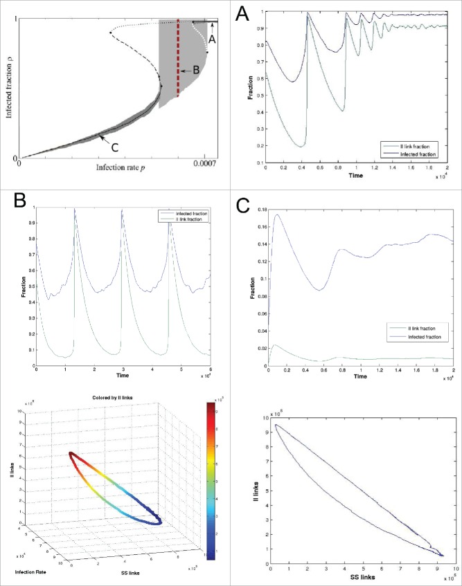
Although the behavior of this model is inherently complex (see the bifurcation diagram in Figure 1A, reproduced by permission),¹⁶ it has been previously established that the system-level dynamics of a sufficiently large network can be captured by just 3 macroscopic observables: the number of infected nodes ${\displaystyle i}$, the number of SS-links ${\displaystyle l_{SS}}$ and the number of II-links ${\displaystyle l_{II}}$. These variables suffice to describe long-term aggregate dynamical behavior types exhibited by the system, since the values of other variables (higher order moments of the network state) quickly become slaved to (functions of) these 3 and do not contribute extra degrees of freedom over long timescales. As the infection parameter ${\displaystyle p}$ varies, one can observe stationary states as well as coarsely oscillatory dynamics, and even coexistence between the 2 (associated with an apparent subcritical coarse Hopf bifurcation).²⁰ In this paper we will show how to extract the relevant observables responsible for the dynamics of the system without making use of any prior knowledge about their suitability. This will be accomplished by first constructing a suitable similarity measure for quantifying graph differences, and secondly, by applying DMAPS on ensembles of graphs resulting from the dynamic simulation of the model's evolution.

Figure 2.

Schematic of the adaptive SIS model evolution: the 3 substeps constituting one SIS evolution timestep. (A) The initial graph at time t. (B) Each infected node recovers with probability r, becoming susceptible. (C) The disease spreads along SI-links with probability p, infecting susceptible nodes. (D) With probability w, each SI-link is broken and a new SS-link is created. (E) The final graph at t+1. Broken links and nodes that change status between steps are colored in red, while rewired links are colored in green.

Figure 1.

(Top left) Model bifurcation diagrams wrt. the infection rate parameter p (reprinted with permission).¹⁶ (A) The system evolves to a stable stationary state for p = 0.00073. (B) Oscillatory behavior indicating a (coarse) limit cycle at p = 0.0006. (C) Stable stationary state for p = 0.0003. Bottom graphs indicate the relationship between i, l_SS, and l_II over the course of one complete oscillation for p = 0.0006. Model parameters: (r, w₀, N, L) = (0.0002, 0.03, 10⁵, 10⁶).

A Brief Discussion of Dimensionality Reduction

Analysis of the dynamics of this epidemic model, especially as the size of the network grows, is hindered by its size and complexity. Not only are there many nodes to keep track of over thousands of time steps, but each step is also comprised of a number of different (stochastic) actions. These factors combine to make systematic exploration of such a system computationally intractable; one may only execute and observe many different scenarios computationally (different initial networks, node states, and parameter values). Additionally, it is not clear which variables, or indeed even how many, play a determining role in summarizing long-term system behavior. This motivates the development of an algorithmic approach to identifying the crucial features of the system. Not only will these important features themselves aid in better understanding the problem and in summarizing its behavior, but they could also be used in an Equation-Free framework to enable the sort of analysis typically reserved for simpler systems (e.g. a few mean-field ODEs). Below, we present our first step toward this goal: the use of the DMAPS data mining technique to identify the important observables in the SIS model from simulation datasets.

Principal Component Analysis and Diffusion Maps

Given a data set ${\displaystyle \left\{x_1,x_2,\dots ,x_N\right\}}$ (with each ${\displaystyle x_i\in {\Re }^n}$), several approaches exist to uncover a lower-dimensional description ${\displaystyle \left\{y_1,y_2,\dots ,y_N\right\} }$ of the data, where ${\displaystyle y_i\in {\Re }^n}$ and ${\displaystyle p<<n}$. Perhaps the best-known method for achieving this is Principal Component Analysis (PCA),¹² illustrated in Figure 3. Unfortunately, PCA assumes the data lies on, or around, a linear subspace, whereas data points generally lie on nonlinear manifolds. To circumvent this limitation we turn to the nonlinear dimensionality reduction technique of Diffusion Maps (DMAPS).¹³ The algorithm is outlined below.

Figure 3.

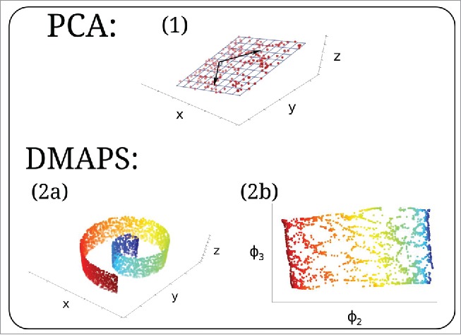
(1) PCA uncovers the linear relationship (2-dimensional blue grid spanned by 2 black arrows) within a noisy data set of 3-dimensional points lying approximately on a plane (red dots). (2a) Three-dimensional data on a nonlinear, curved surface. Color denotes arclength. (2b) DMAPS embedding uncovering a 2-dimensional parameterization of the dataset. Color denotes arclength from (2a).

Given ${\displaystyle N}$ vectors ${\displaystyle \left\{x_1,x_2,\dots ,x_N\right\}}$ in ${\displaystyle {\Re }^n}$, we form an ${\displaystyle N\times N}$ matrix ${\displaystyle W}$ defined as:

$${\displaystyle W_{ij}=exp\left(-\frac{d{\left(x_i,x_j\right)}^2}{{ϵ}^2}\right),}$$

where ${\displaystyle d\left(x_i,x_j\right)}$ is a measure of the distance (“dissimilarity”) between points ${\displaystyle x_i}$ and ${\displaystyle x_j}$, and ${\displaystyle ϵ}$ represents the neighborhood in which we consider ${\displaystyle d\left(x_i,x_j\right)}$ to “meaningfully” capture differences between the data. By defining the diagonal matrix ${\displaystyle D_{ii}={\displaystyle \sum }_j{W}_{ij}}$, we can create a new row-stochastic matrix ${\displaystyle A=D^{-1}W.}$ The entries of ${\displaystyle A}$ can be viewed as defining a random walk over the dataset. The first few eigenvectors of this random walk process represent an efficient parameterization of the original high-dimensional data set. We denote the k-dimensional diffusion map embedding at time ${\displaystyle t}$ as the transformation:

$${\displaystyle {\text{Φ}}_t^{\left(k\right)}=\left({\lambda }_2^t{\varphi }_2, {\lambda }_3^t{\varphi }_3, \dots , {\lambda }_{k+1}^t{\varphi }_{k+1}\right), }$$

where ${\displaystyle {\lambda }_i}$ and ${\displaystyle {\varphi }_i}$ are the i^th eigenvalue and eigenvector respectively, ordered by decreasing magnitude; throughout this paper we set ${\displaystyle t=0}$.

By simulating a diffusion process over the dataset, DMAPS will reveal the underlying low-dimensional nonlinear structure. This is illustrated in Figure 3, where the algorithm is applied to a collection of points ${\displaystyle \left\{x_1,x_2,\dots ,x_N\right\}}$, ${\displaystyle x_i\in {\Re }^3}$ that lie on a curved surface (a “Swiss roll”). The result is a concise, 2-dimensional embedding of the data into ${\displaystyle \left\{y_1,y_2,\dots ,y_N\right\}}$, ${\displaystyle y_i\in {\Re }^{\mathrm{n}}}$.

Similarities between Different Networks

In order to simulate diffusion over the data set, DMAPS requires a scalar distance between 2 data points, ${\displaystyle d\left(x_i,x_j\right)}$. When each point ${\displaystyle x_i}$ is a vector in ${\displaystyle {\Re }^n}$ as in our examples in Figure 3, the Euclidean distance between points is often sufficient. However, in the dataset we investigate below, each point ${\displaystyle x_i}$ is not a vector, but actually a graph (or network), which we represent as ${\displaystyle G_i}$.

The literature contains a number of ways of quantifying the distance between 2 graphs, ${\displaystyle d\left(G_i,G_j\right)}$, for example by measuring how easily ${\displaystyle G_i}$ can be transformed into ${\displaystyle G_j}$ (Graph Edit Distance), or by comparing random walks on the graphs (spectral distance).^21-24 Such distances, however, were found to be computationally intractable for all but very small graphs, which often exhibit much simpler dynamics due to their size. It is therefore important to construct (if possible) a dissimilarity measure that is easily computable on large graphs and has the advantage of being applicable to models with much more complex dynamics. For this reason, we use a different approach for quantifying graph similarity, which is seen here to still be informative while markedly more computationally efficient. Extending previous work on unlabeled graphs,^25,26 we construct a motif-based distance measure for labeled graphs in the following way: we consider 2 graphs to be similar if they share similar numbers of certain features. More precisely, we define a list of ${\displaystyle k}$ subgraphs ${\displaystyle S=\left\{s_1,s_2,\dots ,s_k\right\}}$, such as the single edge, the 2 connected edges, the triangle shown in Figure 4 etc. Then we record how many times each subgraph appears in our input graph in a vector ${\displaystyle v_i=\left\{c_1^i,c_2^i,\dots ,c_k^i\right\}}$, where ${\displaystyle c_j^i}$ is the number of times subgraph ${\displaystyle s_j}$ was found in input graph ${\displaystyle G_i}$. This process maps each graph to a vector of subgraph densities, the counts ${\displaystyle G_i\to v_i, v_i=\left\{c_1^i,c_2^i,\dots ,c_k^i\right\}}$ in ${\displaystyle {\Re }^k}$, thus embedding the graph as a point in ${\displaystyle {\Re }^k.}$ We then use these k-long vectors (k-dimensional points) as the input to DMAPS, and use the Euclidean distance between them as our notion of graph similarity. Thus ${\displaystyle d\left(G_i,G_j\right)=v_i-v_j}$. Figure 4 presents a schematic illustrating this subgraph-enumeration process.

Figure 4.

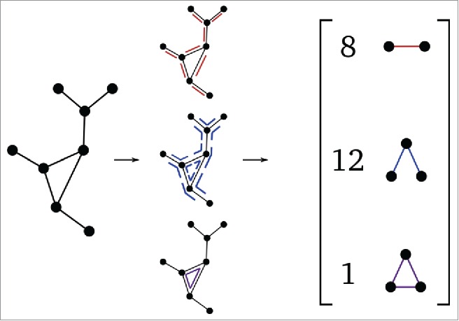
Illustration of the subgraph-enumeration process with an unlabeled input graph.

In the SIS model, we are actually working with labeled graphs, since each node has one of 2 labels – susceptible (S) or infected (I). It is inappropriate to simply ignore network labels, since networks with the same connectivity, but with different node labels, can behave in extremely different ways and should thus be considered dissimilar. To overcome this issue, for a given labeled graph ${\displaystyle G}$ we choose to consider 3 separate unlabeled subgraphs ${\displaystyle G_0, G_S}$ and ${\displaystyle G_I}$. Here ${\displaystyle G_0}$ is the initial graph ${\displaystyle G}$ without node labels and ${\displaystyle G_S}$, ${\displaystyle G_I}$ the unlabeled subgraphs obtained (induced) by only considering the S, or the I nodes respectively. We will represent each overall labeled graph by the concatenation of the 3 count vectors ${\displaystyle v_0, v_I, v_S}$ into ${\displaystyle v={[v_0 v_I v_S]}^T}$, again using the Euclidian norm to quantify (dis)similarity between them. Note that we scale the subgraph counts so that we really measure a “density” of ${\displaystyle s}$ in ${\displaystyle G}$, given by:

$${\displaystyle \rho \left(G,s\right)={\left(\begin{array}{l}n\\ k\end{array}\right)}^{-1}{\displaystyle \sum }_{\text{Φ}:\left[k\right]\to \left[n\right]}1\left[\forall i,j\in k:H\left(i,j\right)=G\left(\text{Φ}\left(i\right),\text{Φ}\left(j\right)\right)\right],}$$

where ${\displaystyle n}$ is the number of nodes in ${\displaystyle G}$, ${\displaystyle k}$ is the number of nodes in ${\displaystyle s}$, ${\displaystyle \text{Φ}}$ is an injection from the first ${\displaystyle k}$ integers to the first ${\displaystyle n}$, and ${\displaystyle 1}$ is an indicator function which takes the value 1 when subgraph ${\displaystyle s}$ has been located in ${\displaystyle G}$. The subgraph enumeration procedure in the case of labeled nodes is illustrated in Figure 5.

Figure 6.

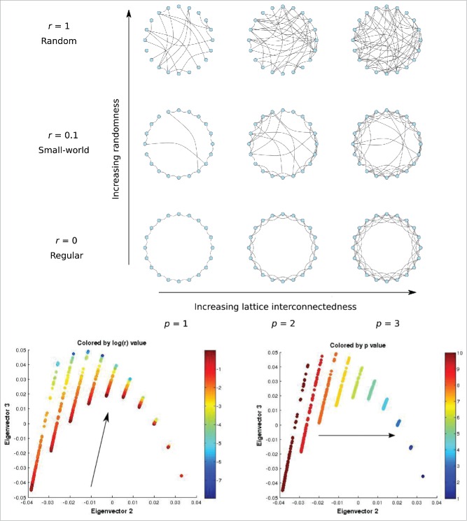
Above: The Watts-Strogatz Model and its construction parameters: The value of r denotes the probability of long-distance rewiring with r = 0 denoting a regular lattice, r < 1 a small-world graph, and r = 1 an Erdős–Rényi random graph. The value of p quantifies how interconnected the initial lattice is, being the number of neighboring nodes each node connects to. Below: Second versus third eigenvector (Φ₂ – Φ₃) colored by log(r) (left) and p (right). The visual linear independence of the directions of change of log(r) and p indicate that the (Φ₂, Φ₃) coordinates form a bijection with (a reparametrization of) the construction parameters (r, p). An ϵ of 0.1 was used in our DMAPS computations.

Figure 7.

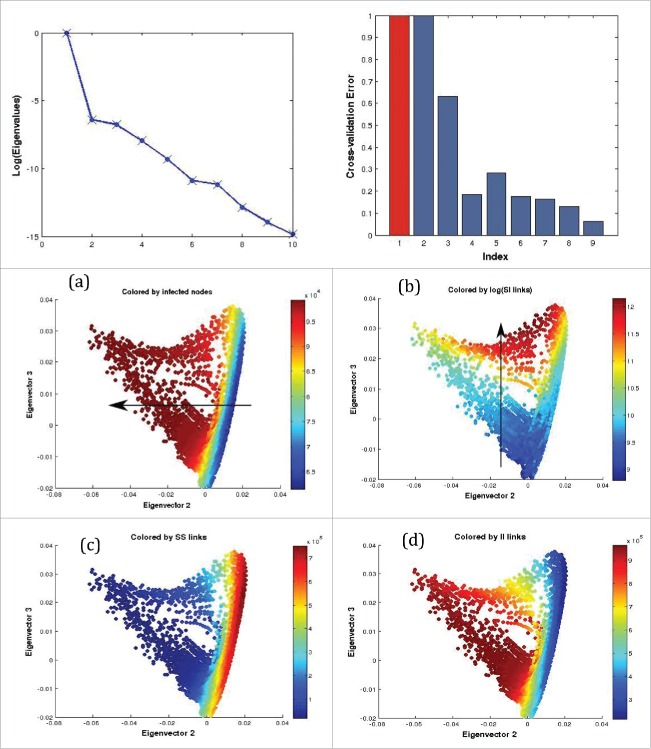
Coarse variable detection: Top Left: The leading eigenvalues of the random walk matrix are plotted. Top Right: Computational criterion suggesting that the first 2 nontrivial eigendirections suffice (the one in red is the trivial one, and the fourth is much less important than the second and third). The x and y coordinates of the middle and bottom row figures indicate the components of each datum, representing a graph, in the second and third eigenvectors of the random walk matrix. Each point is also colored by the number of (a) infected nodes i, (b) log(SI-links), (c) SS-links, and (d) II-links found in the corresponding graph. A comparison between (a) and (b) suggests linear independence between i and log(l_SI). An ϵ of 70 was used.

Figure 8.

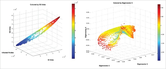
Coarse Variable Dependencies: An illustration of the relationship between l_SS, l_SI, and i in the diffusion map data set. The two-dimensional nature of the manifold indicates that the number of SS links can be thought of as a function, on the data, of i and l_SI, and is thus not necessary as an independent macro-variable.

Figure 5.

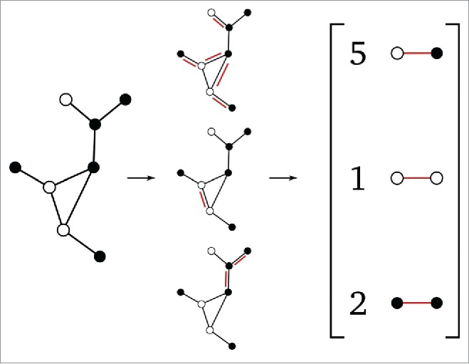
Illustration of the subgraph-enumeration process with a labeled input graph. In this case, we must discriminate between differently labeled subgraphs.

An Unlabeled Graph Example: The Watts-Strogatz Model

To validate the applicability of the above approach/graph similarity measure on graph objects, we used the Watts-Strogatz (WS) network generation model to construct a graph object data set on which to apply DMAPS. For a fixed graph size, the WS model relies on 2 parameters to generate a so-called small-world network output.¹⁹ The first parameter ${\displaystyle p}$ is initially used to generate a 2-dimensional lattice where each vertex is connected to all of its neighbors situated a distance at most ${\displaystyle p}$ away. For each vertex in the graph, we choose the edge that connects it to its nearest neighbor and, with probability ${\displaystyle r}$, rewire this edge to connect with a vertex chosen uniformly at random from the graph. This procedure is repeated, each time considering the edge that connects the next closest neighbor to the vertex in question until all edges have been considered once, with no duplicate edges allowed. The resulting graph is considered the output of the model. The networks produced by this model exhibit various qualitatively different properties as its “generating parameters” vary. For ${\displaystyle r=1}$ the model reduces to generating an Erdős–Rényi random graph ${\displaystyle G\left(n,p\right)}$: a graph of size ${\displaystyle n}$ for which the probability that any 2 vertices are connected is ${\displaystyle p}$. On the other hand, for ${\displaystyle r=0}$ the graph remains a regular lattice, with no random changes in its topology. Lastly, for intermediate values of ${\displaystyle r}$ we get many local connections between adjacent nodes and few edges between far away nodes, which is a defining characteristic of small-world networks.

The WS algorithm was used to generate ${\displaystyle n=2000}$ different small-world graphs, each with ${\displaystyle n=100}$ vertices. For each such graph ${\displaystyle G_i\left(p_i, r_i\right)}$, we generated uniformly at random the 2 variables ${\displaystyle r_i \sim \text{unif}\left[0,1\right]}$ and ${\displaystyle p_i \sim \text{unif}\left[0,1\right]}$. We thus are confident that, by construction, this is a 2-parameter set of graph data, parametrized by the generating parameters ${\displaystyle p}$ and ${\displaystyle r}$. The diffusion map embedding was then constructed by using the graph similarity measure defined above. It was found (Fig. 6) that the first 2 principal DMAP eigenvectors ${\displaystyle {\varphi }_2}$ and ${\displaystyle {\varphi }_3}$ were sufficient to represent the data. This is confirmed by the 2 dimensional nature of the ${\displaystyle \left({\varphi }_2-{\varphi }_3\right)}$ manifold. When considering the values of ${\displaystyle p_i}$ and ${\displaystyle r_i}$ of the various data points (the various graphs) that lie on this 2-dimensional manifold, it can be observed that they vary in directions visually independent of each other. This strongly suggests that the transformation ${\displaystyle f:\left({\varphi }_2,{\varphi }_3\right) \to \left(r,p\right)}$ has a nonsingular Jacobian matrix, which in turn implies that the transformation is bijective – the 2 variable pairs are one-to-one with each other, and they each constitute useful coordinates (Figure 6, below) for the network dataset. This means that DMAPS discovered a reparameterization of the 2 parameters ${\displaystyle r}$ and ${\displaystyle p}$, which in this case were known in advance to be (by construction) the parameters that define this data set. This serves as a validation for the DMAPS approach and the chosen graph similarity measure since, by only examining a dataset generated by the WS model, the technique was able to “learn” that only 2 features mattered, and that the 2 features were one-to-one with the construction parameters ${\displaystyle \left(r,p\right)}$ that here were a priori known.

SIS Model Results

In order to identify the coarse variables that parametrize the dynamics of the adaptive SIS model, DMAPS were implemented on a graph data set sampled from the SIS model evolution. This dataset was generated by systematically sampling graph objects from the SIS model simulation over time from various parameters/initial conditions, with each simulation leading to different long-term dynamical behavior. The principal directions, represented by the leading diffusion map coordinates, identify the important variables that define the model's evolution over time. Since the set of coarse variables ${\displaystyle \left(i, l_{II}, l_{SS}\right)}$ are known to be central to the model's evolution, their relationship with the derived principal directions was investigated.¹⁶

More specifically, the system is known to undergo a Hopf bifurcation to periodic solutions as the parameter ${\displaystyle p}$ varies around ${\displaystyle \left(p, r, w_0\right)\approx \left(0.00071,0.0002,0.06\right)}$ and graph objects at parameter values around this bifurcation point were sampled to create a data set of ${\displaystyle N = 6000}$ graphs ${\displaystyle {\left\{G_i\right\}}_{i=1}^N}$. After the graphs were sampled, the DMAPS procedure detailed above was applied, with our labeled graph similarity measure (Fig. 7). An analysis of the relationship between the diffusion map coordinates indicates a 2-dimensional embedding in the first 2 principal directions ${\displaystyle {\varphi }_2, {\varphi }_3}$. Furthermore, an investigation of the relationship between ${\displaystyle {\varphi }_2}$ and ${\displaystyle {\varphi }_3}$ with other diffusion map coordinates demonstrates that no new direction is captured by higher order eigenvectors, something that strongly implies that the manifold on which the dataset lies is indeed 2-dimensional. This is achieved by performing linear regression, with a suitable kernel, on the eigenvectors, and checking whether each ${\displaystyle {\varphi }_i}$ can be accurately reconstructed using the rest, quantified as cross-validation error.²⁷ This measure is high for eigenvectors characterized by unique directions, and low for higher harmonics and noise. It has the added benefit that it can be used to compare many eigenvectors, not limiting it only to the first few.

Motivated by the evidence that the ${\displaystyle ({\varphi }_2,{\varphi }_3)}$ manifold fully captures all independent directions in the data set, we look at the relationship between these 2 principal directions and the coarse variables ${\displaystyle \left(i, l_{II}, l_{SS}\right)}$, known to encapsulate the long-term dynamics of this system. This can be investigated by visually studying the embedding of the coarse variables in diffusion map space and by using the cross-validation algorithm defined above. Looking at the relationship between these 3 variables in our dataset, it can be noticed that they actually span 2 (and not 3 different) dimensions, which can be garnered by their 2 dimensional embedding in ${\displaystyle {\Re }^3}$. Thus, we are actually looking for 2 principal directions, motivating the definition of ${\displaystyle l_{SI}=L- \left(l_{II}+ l_{SS}\right),}$ the total number of SI-links, as a compound variable. This is done without introducing or removing any information from the system, as the total number of edges is constant throughout. We consider ${\displaystyle \text{log}\left(l_{SI}\right)}$ as a candidate macro-variable, since we are interested in finding a bijective relationship between ${\displaystyle ({\varphi }_2,{\varphi }_3)}$ and ${\displaystyle \left(i, l_{SI}\right)}$.

By inspecting (see Figure 8) the relative directions of ${\displaystyle i}$ and ${\displaystyle \text{log}\left(l_{SI}\right)}$ in the 2 dimensional embedding of ${\displaystyle ({\varphi }_2,{\varphi }_3)}$, it becomes apparent that they are transverse to each other, with the former varying roughly from left to right and the latter from top to bottom. Such an observation is strong evidence that the Jacobian of the transformation ${\displaystyle f:\left({\varphi }_2,{\varphi }_3\right) \to \left(i, l_{SI}\right)}$ is nonsingular on this data set, much in the same manner as for the Watts-Strogatz graph ensembles. Thus, we can conclude that the directions of change on the ${\displaystyle {\varphi }_2-{\varphi }_3}$ manifold represented by changing ${\displaystyle i}$ and ${\displaystyle l_{SI}}$, respectively, are independent of each other, and that they are reparametrizations of the principal eigenvectors. Similar results are obtained if we consider ${\displaystyle l_{SI}}$ instead of ${\displaystyle \text{log}\left(l_{SI}\right)}$. These observations imply that the diffusion map technique has been successful in identifying, up to reparameterization, the variables found in ref. 16 as responsible for the long term dynamics of the model. Furthermore, we were able to confirm that the long-term dynamics of this model really depend on only 2 macro-variables, the total number of infected nodes ${\displaystyle i}$ and the total number of SI-links ${\displaystyle l_{SI}}$.

In addition, there was no need to take any a priori knowledge about the model's specifics into account when isolating the important variables. Instead, we required the development of a suitable similarity measure between labeled graphs, which can be generalized for use with other problems (models, datasets) that exhibit completely different dynamic behavior. This generalization of feature extraction for high-dimensional systems can assist in developing a framework for isolating the coarse variables that define graph-based data sets without resorting to approaches that only rely on intuition about the specific model.

Conclusion

The use of networks in the modeling of real-world phenomena is particularly suited to modeling the spread of an epidemic through a population represented as a network of geographic/social connections. In this paper, the suitability of data mining techniques for extracting the important macro-variables describing the evolution of network connectivity from an adaptive SIS model were investigated, based on 2 concepts. Firstly, a (dis)similarity measure for graph objects was constructed; secondly, it was used with the DMAPS nonlinear data-mining procedure. In particular, we needed to define a (dis)similarity measure between different labeled graphs, as they arise in the course of the epidemic model simulation. It should be noted that this method is generalizable to any labeled graph with distinct labels, and can be utilized regardless of the overarching process defining graph evolution. Future work in this area should investigate the suitability of other graph similarity measures for use within the DMAPS framework. Moreover, this approach is not DMAPS-specific. Indeed, other non-linear data mining techniques are expected to yield similar results, provided they use the aforementioned dissimilarity measure.

In addition, the long-term dynamics of a particular adaptive SIS model were explored, which allowed us to verify the suitability of the constructed metric for use with graph object datasets. This yields 2 interconnected results. Firstly, the DMAP procedure was able to demonstrate that the system is inherently macroscopically two-dimensional, with the 2 independent directions in the data set being represented by the first 2 nontrivial Diffusion Map eigenvectors. This result is consistent with previous knowledge about the dimensionality of the model's dynamics, and is strong evidence that the DMAP framework, using the similarity measure we constructed, can be readily applied to graph object data sets to extract meaningful reduced parametrizations of the underlying behavior.

Furthermore, we were also able to link the principal diffusion map coordinates with previously known coarse variables capable of describing this system. By inspection of the embeddings in diffusion space, it was verified that a bijection exists between 2 of these coarse variables and the 2 leading diffusion map coordinates. This means that the DMAP was not only able to learn the inherent dimensionality of the dataset, but that it was also able to extract a reparameterization of variables known to fully specify this model; what is unfortunate, is that the variables of this reparametrization have no obvious unique, easily explainable physical meaning.

This modeling exercise clearly shows that modern data mining techniques for data in the form of high-dimensional evolving vectors can be extended to data in the form of large evolving graphs (labeled or unlabeled). This holds promise for the analysis of data from epidemics on realistic adaptive networks, and for general adaptive network evolution problems. What is more important and more promising, however, is that these databased coarse descriptors can be used, in an equation-free framework^8,9, to implement accurate reduced model computations for the epidemic dynamics, in which the variables used to describe the systems-level network behavior are the ones obtained from data mining. This data-driven model reduction approach can be introduced as a “wrapper algorithm” around brief bursts of detailed, fine scale simulation; we believe that the approach holds real promise in enabling systems level analysis, simulation and control of detailed, realistic epidemic dynamics.

Disclosure of Potential Conflicts of Interest

No potential conflicts of interest were disclosed.

Funding

This work was partially supported by the US National Science Foundation. The work of IGK and AK was partially supported by the Technische Universität München- Institute for Advanced Study, funded by the German Excellence Initiative and the European Union Seventh Framework Programme under grant agreement n° 291763.

References

- 1.Gross T, D'Lima CJ, Blasius B. Epidemic dynamics on an adaptive network. Phys Rev Lett 2006; 96:208701; PMID:16803215; http://dx.doi.org/ 10.1103/PhysRevLett.96.208701 [DOI] [PubMed] [Google Scholar]
- 2.Pastor-Satorras R, Castellano C, Van Mieghem P, Vespignani A. Epidemic processes in complex networks. Rev Mod Phys 2015; 87:925-79; http://dx.doi.org/ 10.1103/RevModPhys.87.925 [DOI] [Google Scholar]
- 3.Van Segbroeck S, Santos FC, Pacheco JM. Adaptive contact networks change effective disease infectiousness and dynamics. PLoS Comput Biol 2010; 6:e1000895; PMID:20808884; http://dx.doi.org/ 10.1371/journal.pcbi.1000895 [DOI] [PMC free article] [PubMed] [Google Scholar]
- 4.Zhou J, Xiao G, Cheong SA, Fu X, Wong L, Ma S, Cheng TH. Epidemic reemergence in adaptive complex networks. Phys Rev E Stat Nonlin Soft Matter Phys 2012; 85:036107; PMID:22587149; http://dx.doi.org/ 10.1103/PhysRevE.85.036107 [DOI] [PubMed] [Google Scholar]
- 5.Colizza V, Barrat A, Barthelemy M, Vespignani A. The modeling of global epidemics: Stochastic dynamics and predictability. B Math Biol 2006; 68:1893-921; http://dx.doi.org/ 10.1007/s11538-006-9077-9 [DOI] [PMC free article] [PubMed] [Google Scholar]
- 6.Wang B, Cao L, Suzuki H, Aihara K. Epidemic spread in adaptive networks with multitype agents. J Phys a-Math Theor 2011; 44:035101; http://dx.doi.org/ 10.1088/1751-8113/44/3/035101 [DOI] [Google Scholar]
- 7.Eubank S, Guclu H, Anil Kumar VS, Marathe MV, Srinivasan A, Toroczkai Z, Wang N. Modelling disease outbreaks in realistic urban social networks. Nature 2004; 429:180-4; PMID:15141212; http://dx.doi.org/ 10.1038/nature02541 [DOI] [PubMed] [Google Scholar]
- 8.Kevrekidis IG, Gear CW, Hyman JM, Kevrekidis PG, Runborg O, Theodoropoulos C. Equation-Free, Coarse-Grained Multiscale Computation: Enabling Mocroscopic Simulators to Perform System-Level Analysis. Commun Math Sci 2003; 1:715-62; http://dx.doi.org/ 10.4310/CMS.2003.v1.n4.a5 [DOI] [Google Scholar]
- 9.Kevrekidis IG, Gear CW, Hummer G. Equation-free: The computer-aided analysis of complex multiscale systems. AIChE Journal 2004; 50:1346-55; http://dx.doi.org/ 10.1002/aic.10106 [DOI] [Google Scholar]
- 10.Tsoumanis AC, Rajendran K, Siettos CI, Kevrekidis IG. Coarse-graining the dynamics of network evolution: the rise and fall of a networked society. New J Phys 2012; 14:083037; http://dx.doi.org/ 10.1088/1367-2630/14/8/083037 [DOI] [Google Scholar]
- 11.Siettos CI. Equation-Free multiscale computational analysis of individual-based epidemic dynamics on networks. Applied Mathematics and Computation 2011; 218:324-36; http://dx.doi.org/ 10.1016/j.amc.2011.05.067 [DOI] [Google Scholar]
- 12.Jolliffe IT. Principal component analysis. New York: Springer, 2002. [Google Scholar]
- 13.Coifman RR, Lafon S. Diffusion maps. Appl Comput Harmon A 2006; 21:5-30; http://dx.doi.org/ 10.1016/j.acha.2006.04.006 [DOI] [Google Scholar]
- 14.Tenenbaum JB, de Silva V, Langford JC. A Global Geometric Framework for Nonlinear Dimensionality Reduction. Science 2000; 290:2319-23; PMID:11125149; http://dx.doi.org/ 10.1126/science.290.5500.2319 [DOI] [PubMed] [Google Scholar]
- 15.Gross T, Blasius B. Adaptive coevolutionary networks: a review. J R Soc Interface 2008; 5:259-71; PMID:17971320; http://dx.doi.org/ 10.1098/rsif.2007.1229 [DOI] [PMC free article] [PubMed] [Google Scholar]
- 16.Gross T, Kevrekidis IG. Robust oscillations in SIS epidemics on adaptive networks: Coarse graining by automated moment closure. Epl-Europhys Lett 2008; 82:38004; http://dx.doi.org/ 10.1209/0295-5075/82/38004 [DOI] [Google Scholar]
- 17.Sayama H, Pestov I, Schmidt J, Bush BJ, Wong C, Yamanoi J, Gross T. Modeling complex systems with adaptive networks. Comput Math Appl 2013; 65:1645-64; http://dx.doi.org/ 10.1016/j.camwa.2012.12.005 [DOI] [Google Scholar]
- 18.Huepe C, Zschaler G, Do A-L, Gross T. Adaptive-network models of swarm dynamics. New J Phys 2011; 13:073022; http://dx.doi.org/ 10.1088/1367-2630/13/7/073022 [DOI] [Google Scholar]
- 19.Watts DJ, Strogatz SH. Collective dynamics of ‘small-world’ networks. Nature 1998; 393:440-2; PMID:9623998; http://dx.doi.org/ 10.1038/30918 [DOI] [PubMed] [Google Scholar]
- 20.Holmes P, Lumley JL, Berkooz G, Rowley CW. Turbulence, coherent structures, dynamical systems and symmetry, 2nd Edition. Cambridge Monographs on Mechanics, Cambridge: Cambridge University Press [Google Scholar]
- 21.Bunke H, Shearer K. A graph distance metric based on the maximal common subgraph. Pattern Recogn Lett 1998; 19:255-9; http://dx.doi.org/ 10.1016/S0167-8655(97)00179-7 [DOI] [Google Scholar]
- 22.Gao X, Xiao B, Tao D, Li X. A survey of graph edit distance. Pattern Anal Appl 2010; 13:113-29; http://dx.doi.org/ 10.1007/s10044-008-0141-y [DOI] [Google Scholar]
- 23.Papadimitriou P, Dasdan A, Garcia-Molina H. Web graph similarity for anomaly detection. J Internet Serv Appl 2010; 1:19-30; http://dx.doi.org/ 10.1007/s13174-010-0003-x [DOI] [Google Scholar]
- 24.Vishwanathan SVN, Schraudolph NN, Kondor R, Borgwardt KM. Graph kernels. J Mach Learn Res 2010; 11:1201-42 [Google Scholar]
- 25.Xiao Y, Dong H, Wu W, Xiong M, Wang W, Shi B. Structure-based graph distance measures of high degree of precision. Pattern Recogn 2008; 41:3547-61; http://dx.doi.org/ 10.1016/j.patcog.2008.06.008 [DOI] [Google Scholar]
- 26.Rajendran K, Kevrekidis IG. Analysis of data in the form of graphs. arXiv preprint arXiv:13063524 2013. [Google Scholar]
- 27.Dsilva CJ, Talmon R, Gear CW, Coifman RR, Kevrekidis IG. Data-Driven Reduction for Multiscale Stochastic Dynamical Systems. arXiv preprint arXiv:150105195 2015. [Google Scholar]