Monitoring Antimicrobial Resistance in the Food Supply Chain and Its Implications for FDA Policy Initiatives

Abstract

In response to concerning increases in antimicrobial resistance (AMR), the Food and Drug Administration (FDA) has decided to increase veterinary oversight requirements for antimicrobials and restrict their use in growth promotion. Given the high stakes of this policy for the food supply, economy, and human and veterinary health, it is important to rigorously assess the effects of this policy. We have undertaken a detailed analysis of data provided by the National Antimicrobial Resistance Monitoring System (NARMS). We examined the trends in both AMR proportion and MIC between 2004 and 2012 at slaughter and retail stages. We investigated the makeup of variation in these data and estimated the sample and effect size requirements necessary to distinguish an effect of the policy change. Finally, we applied our approach to take a detailed look at the 2005 withdrawal of approval for the fluoroquinolone enrofloxacin in poultry water. Slaughter and retail showed similar trends. Both AMR proportion and MIC were valuable in assessing AMR, capturing different information. Most variation was within years, not between years, and accounting for geographic location explained little additional variation. At current rates of data collection, a 1-fold change in MIC should be detectable in 5 years and a 6% decrease in percent resistance could be detected in 6 years following establishment of a new resistance rate. Analysis of the enrofloxacin policy change showed the complexities of the AMR policy with no statistically significant change in resistance of both Campylobacter jejuni and Campylobacter coli to ciprofloxacin, another second-generation fluoroquinolone.

INTRODUCTION

Antimicrobial resistance (AMR) is one of the most serious health threats to both animals and humans. Therefore, the mitigation of AMR in animal agriculture is critical for both the agrifood industry and for public health (1, 2). Globally and nationally, there is much attention on developing approaches to mitigate AMR (3, 4, 5, 6). Overuse of antimicrobials contributes to the emergence and proliferation of resistant bacterial strains. Historically, antimicrobials have been administered to livestock and poultry to address animal health as well as for production purposes. In order to slow down the development and proliferation of AMR in food animal agriculture, the Food and Drug Administration (FDA) has initiated a risk mitigation strategy to limit use of medically important antimicrobials to therapeutic uses under veterinary oversight by working with drug companies to change product labels (5, 6).

A key piece of evidence in evaluating the efficacy of this policy is detecting the change in AMR before and after the policy has been implemented. To do so, it is necessary to understand the baseline variation of AMR over time and at different stages of the food supply chain. The most comprehensive information on AMR in United States agriculture is the newly public data from the National Antimicrobial Resistance Monitoring System (NARMS). NARMS longitudinally monitors resistance of nontyphoidal Salmonella, Campylobacter spp., Escherichia coli, and Enterococcus spp. to a variety of antibiotics (7). Resistance of each isolate is reported as a MIC which can then be transformed into a susceptible/resistance value based on whether this MIC exceeds a given resistance threshold. Where defined, NARMS uses the clinical breakpoints published by the Clinical and Laboratory Standards Institute (CLSI) to interpret MIC values as susceptible or resistant and uses epidemiological cutoffs where clinical breakpoints are not defined (8). The clinical breakpoints defined by the CLSI are typically determined by the probability of therapeutic failure in humans and are intended to guide clinical decision making (9). Epidemiological cutoffs represent the level of resistance which demarcates the boundary between the wild-type population and resistant mutants. They are determined as the value that separates the main part of the MIC distribution from the upper tail (9).

The historical trends of AMR have been preliminarily explored in the annually published NARMS reports. These reports focused on resistance proportions and modeled slaughter and retail separately. Dichotomizing MIC values, however, risks a loss of information (10, 11). Dichotomization of MIC results also cannot detect shifts from low to high resistance levels, which provide an early warning for increasing resistance in a population. Clinical breakpoints may also shift over time to reflect changes in AMR interpretation, reporting, and methods, resulting in changes in reported resistance proportions not related to changes in population (12, 13). Pulsed-field gel electrophoresis (PFGE) profiles of Campylobacter and Salmonella from broiler flocks found identical clones from primary production through slaughter to retail products (14, 15), indicating that there is a connection between resistance levels at various stages of the food supply chain.

The objectives of this study were to evaluate the baseline trend and variations in the NARMS data and provide useful information to improve data collection, analysis, and synthesis in the national AMR monitoring system. To achieve these objectives, we extended the annual NARMS reports by examining both percent resistance and mean MIC values. Moreover, we considered each of these values simultaneously at the slaughter and retail stages. We examined the structure of the variation in resistance within/between years and across geographic regions. Using this baseline, we estimated how much data must be collected to be able to determine if the change in FDA policy did indeed have an effect. Finally, using this information we examined the impact of a previous change in FDA antimicrobial policy, removing approval of enrofloxacin for use in poultry water in 2005.

MATERIALS AND METHODS

The data set.

The NARMS data were obtained from the FDA website (7). The data files for Retail Meats, HACCP 1997-2005, HACCP 2006-2013, and Cecal were combined and stored in an SQLite database. MIC values were log₂ transformed, which reduced skewness (16). The MICs of isolates susceptible to the lowest antibiotic concentration tested were taken to be this lowest concentration, and the log₂-transformed MICs of isolates resistant to the highest concentration tested were increased incrementally by 1.

Although we examined many different combinations of microbes, hosts, and antibiotics, we focus here on chicken as the host and examined resistance of Campylobacter jejuni to tetracycline, Campylobacter coli to erythromycin, Salmonella enterica serovar Typhimurium to ampicillin, and Escherichia coli to streptomycin. In accordance with NARMS guidelines, resistance for all Campylobacter and E. coli-streptomycin tests was determined using epidemiological cutoffs, and resistance for S. Typhimurium-ampicillin was determined based on the CLSI breakpoint (17). Chicken data had the most consistent data across all time points and stages. Analyzed drugs were chosen not only for their significance in human medicine but also for their importance in veterinary medicine and extent of use in food production (18). Bacteria were selected for their significance as pathogens, number of observations, and MIC distribution patterns. The time frame of 2004 to 2012 was chosen because both slaughter and retail data for chicken were available during this time period (retail data were first available in 2004, and 2012 was the last year the HACCP slaughter data were available), which made the stage effect analysis possible. Sample size per year and stage ranged from 21 to 2,232 tests.

MIC distributions over time and across stages.

In order to obtain a baseline understanding of AMR changes over time and across different stages of the food supply chain (i.e., slaughter and retail), we began by first exploring the resistance data for each microbe/host/antibiotic combination. Line graphs were used to visualize resistance data, and boxplots were used to visualize the distribution of the MICs.

Generalized linear modeling of resistance.

To quantitatively assess trends in AMR, we constructed models of resistance both as a binary variable using logistic regression and as a continuous variable using linear regression, using log₂ MIC values. To quantitatively assess the sources of variation, we constructed a linear mixed-effect model. All models were implemented using the Python statsmodels package (version 0.6.1) (http://statsmodels.sourceforge.net/index.html). The significance of all coefficients was assessed using a likelihood ratio test.

Modeling resistance prevalence: logistic regression.

Logistic regression was carried out by modeling the log odds of resistance versus nonresistance as a function of stage and year. We chose 2004 retail data as the baseline level. The model is shown in equation 1:

$$\ln \left(\frac{p_{ij}}{1-p_{ij}}\right)=\alpha +{\text{β}}_i+{\text{β}}_{\text{slaughter}}\text{slaughter}+e_{ij}$$ (1)

where α and β are coefficients, i is the index over the years, j is the index over slaughter and retail stages, and slaughter is an indicator variable designating whether the sample came from slaughter or retail. The e term is the error.

To determine the robustness of this analysis to the choice of resistance threshold, C. coli-erythromycin was taken as an example and the regression was carried out using each MIC as a cutoff. The stability of the model was evaluated based on the similarity of the resulting coefficients.

Modeling MIC distribution: linear regression.

As a means of both sidestepping the choice of a breakpoint and adding an additional viewpoint on AMR, MIC was treated as a continuous variable and the mean log₂ MIC was modeled as a linear function of stage and year. The linear model is shown in equation 2.

$${\log }_2{\text{MIC}}_{ij}=\alpha +{\text{β}}_i+{\text{β}}_{\text{slaughter}}\text{slaughter}+e_{ij}$$ (2)

Modeling sources of variation: linear mixed-effect model.

To study the sources of variation in resistance, the log₂ MIC at each stage was modeled separately as a function of a fixed intercept for state and a random intercept for year according to equation 3.

$${\log }_2{\text{MIC}}_{ik}=\text{μ}+{\text{Year}}_i+{\text{State}}_k+e_{ik}$$ (3)

where i is the index over years and k is the index over the states.

Power analysis.

To formally evaluate the effectiveness of the FDA policy change in a manner consistent with the exploratory and regression analyses, we propose a model with a constant base level of resistance around which the yearly levels vary, a period in which the levels change, and then the establishment of a new resistance level (Fig. 1). Under this model, a hypothesis test of mean resistance level before and after the policy change can assess the change in resistance. It is assumed that there is a different amount of variation within years and between years, so the test is carried out on average yearly resistance. This test can be done with either percent resistance or MIC values (19). A power analysis was performed to benchmark the efficacy of this test. Calculating power requires knowledge of the standard deviation, sample size, and magnitude of the effect to be detected. For the t test of mean log₂ MIC, sensible standard deviations were selected by calculating the empirical distribution for the standard deviations of the mean log₂ MIC per year. The number of isolates per year was assumed to be 200, a number generally exceeded in historical data. The current 9 years of data were used as the prepolicy change sample size. Postpolicy change sample sizes were assumed to be between 1 and 10 years. The desired detectable effect was taken to be between 0 and 1 log₂ MIC. Power curves were then plotted according to equation 4.

$$\text{Power}=P(t<t_{\text{critical\_val\_low}})+P(t>t_{\text{critical\_val\_up}})$$ (4)

where t = $\sqrt{{nw}_2}[(\overline{x_1}-\overline{x_2})/s]$ with n − 2 degrees of freedom and noncentrality parameter δ, where δ = $\sqrt{{nw}_1{w}_2}$(μ_diff/σ). t_{critical_val_low} is the α/2 quantile of the central t distribution with n − 2 degrees of freedom, t_{critical_val_up} is the 1 − α/2 quantile of the central t distribution with n − 2 degrees of freedom, n is the total number of observations, and w is the fraction of observations in each sample.

FIG 1.

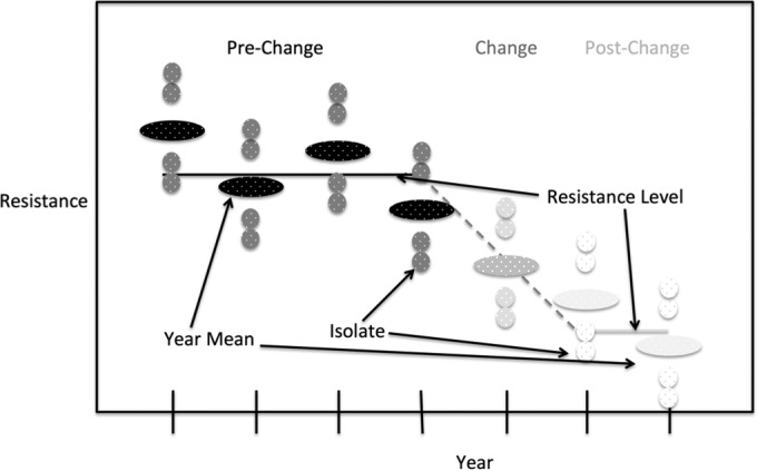
Model of antimicrobial resistance used in evaluating policy changes. It is assumed there is a constant base level of resistance around which the yearly levels vary, a period of change, and then the establishment of a new resistance level.

Resistant/susceptible counts are binomial quantities, so their standard deviations are functions of the proportions. However, because the data come from a mix of conditions, like geographical location, season, and production quality, these proportions are overdispersed with respect to binomial variation, and the standard deviations will also be a function of this overdispersion parameter. Reasonable proportions and overdispersion parameters were obtained by plotting the empirical distribution of each quantity. The number of isolates per year was set to 200, prepolicy change sample size was 9 years, postchange sample size was between 1 and 10 years, and effect sizes were chosen so as to be detectable with such sample sizes. The power curves were then plotted according to equation 5.

$$\text{power}=\mathrm{\Phi }(r{c}_{\text{low}}-\frac{p_2-p_1}{\text{SE}})+1-\mathrm{\Phi }(r{c}_{\text{up}}-\frac{p_2-p_1}{\text{SE}})$$ (5)

where r = $\sqrt{[p(1-p)(1/k_1-1/k_2)]/[p_1(1-p_1)/k_1+p_2(1-p_2)/k_2]}$, standard error $(\text{SE})=\sqrt{\varphi [p_1(1-p_1)/n{k}_1]+p_2(1-p_2)/n{k}_2},\hspace{0.17em}p=(k_1/k)p_1+(k_2/k)p_2\hspace{0.17em}$, Φ is the normal PDF, c is a critical value, k is the number of years in a sample, and ϕ is the overdispersion.

The role of isolate count was determined by calculating power as described for equation 4 but replacing the single standard deviation parameter, s, with the combination of between-year and within-year standard deviations in equation 6.

$$s=\sqrt{{s_{\text{between}}}^2+\frac{{s_{\text{within}}}^2}{n}}$$ (6)

where n is the number of isolates per year. The resulting power was plotted for n between 1 and 2,000, assuming s_between is 0.6, s_within is 3, the prepolicy change sample size was 9 years, the postchange sample size was 5, and the effect size was a 1-fold change in MIC.

During assessment, a power of 0.8 was chosen as the desirable threshold.

Assessing the effect of the change in enrofloxacin policy.

In 2005 the FDA withdrew approval of enrofloxacin in poultry water. Due to this policy change having much the same form as the current policy change, it serves as a useful case study. Since enrofloxacin is metabolized to ciprofloxacin, the analysis focused on the latter antibiotic. We evaluated its resistance using the exploratory analysis, generalized linear models, and t test as in the baseline study. Since the policy change occurred in 2005, we extended to time period under consideration back to 2002.

RESULTS

Analysis of MIC distributions over time and across stages.

Preliminary analysis of the raw data revealed that the trend in AMR was largely dependent on the bacterium-drug combination. In most cases, like C. jejuni-ciprofloxacin, C. jejuni-tetracycline, C. coli-erythromycin, and S. Typhimurium-ampicillin, the average log₂ MIC increased slightly over time (Fig. 2 to 4). In other cases, like E. coli-streptomycin, there was a marked decrease in resistance during the study period (Fig. 5). The relationship between slaughter and retail was also case dependent, with slaughter sometimes higher than retail and retail sometimes higher than slaughter. The distribution of MICs was generally highly skewed, and in many cases the median, first quartile, and even the minimum all coincided. The percent resistance followed the same trend as the log₂ MIC, but with much higher variability.

FIG 2.

Exploratory analysis of Campylobacter jejuni resistance to tetracycline. (A) Boxplots of log₂ MIC values. The lower whisker is the minimum observed MIC in a given year, the lower edge of the box is the first quartile, the line is the median, the square is the mean, the top of the box is the third quartile, and the upper whisker is the maximum. The dashed line indicates the breakpoint between resistant and susceptible isolates. (B) Line graph of percentage of isolates with MIC values above the resistance breakpoint. Sizes of points are proportional to the number of observations in the given year and stage. Sample sizes ranged from 78 to 1,348.

FIG 3.

Exploratory analysis of Campylobacter coli resistance to erythromycin. (A) Boxplots of log₂ MIC values. The dashed line indicates the breakpoint between resistant and susceptible isolates. (B) Line graph of percentage of isolates with MIC values above the resistance breakpoint. Sizes of points are proportional to the number of observations in the given year and stage. Samples sizes ranged from 76 to 693.

FIG 4.

Exploratory analysis of Salmonella Typhimurium resistance to ampicillin. (A) Boxplots of log₂ MIC values. The dashed line indicates the breakpoint between resistant and susceptible isolates. (B) Line graph of percentage of isolates with MIC values above the resistance breakpoint. Sizes of points are proportional to the number of observations in the given year and stage. Samples sizes ranged from 21 to 104.

FIG 5.

Exploratory analysis of Escherichia coli resistance to streptomycin. (A) Boxplots of log₂ MIC values. The dashed line indicates the breakpoint between resistant and susceptible isolates. (B) Line graph of percentage of isolates with MIC values above the resistance breakpoint. Sizes of points are proportional to the number of observations in the given year and stage. Samples sizes ranged from 299 to 2,232.

Logistic modeling.

The logistic model (Table 1) confirmed the results of the exploratory analysis. Both the coefficients themselves and the significant coefficients were dependent on the specific drug-bacterium combination. Although the intercept and at least one of the year coefficients was significant in all cases, which particular year coefficient was significant varied widely. For E. coli-streptomycin, all year coefficients were significant. In C. coli-erythromycin, only the coefficient for 2011 was significant. The coefficient for slaughter was significant for E. coli-streptomycin and S. Typhimurium-ampicillin. It was not significant for C. coli-erythromycin or C. jejuni-tetracycline, not because there was no difference between slaughter and retail but because slaughter was sometimes higher than retail and sometimes lower.

TABLE 1.

Values of coefficients for the logistic regression of resistance on year and stage

Coefficient	Value fora:
	C. coli-erythromycin	C. jejuni-tetracycline	E. coli-streptomycin	S. Typhimurium-ampicillin
α	−2.29*	−0.19*	0.31*	0.81*
β2005	−0.04	−0.03	−0.25*	−0.67*
β2006	−0.28	0.19	−0.54*	−0.06
β2007	0.00	0.23*	−0.65*	−0.37
β2008	0.10	0.21	−0.43*	−0.49*
β2009	−0.64	0.05	−0.63*	−0.13
β2010	−0.88	−0.21	−0.64*	−0.12
β2011	−0.87*	0.05	−0.55*	−0.51*
β2012	0.00	0.16*	−0.82*	−0.59*
βslaughter	0.00	0.03	0.26*	−1.13*

^aAn asterisk indicates significance at an α value of 0.05.

The distribution of MICs (Fig. 6) for C. coli-erythromycin showed that at both slaughter and retail there was one narrow peak above the log₂ MIC cutoff of 5 and a broad peak between −1 and 2. The broad peak between −1 and 2 is likely to represent the MIC distribution for the wild-type isolates, while the isolates with log₂ MIC above 5 are likely to represent the non-wild-type isolates. The sensitivity analysis (Table 2) showed that the model was highly sensitive to the choice of cutoff. For all of the years, the coefficients in the logistic models vary to a large degree with the choice of cutoff. Many of the coefficients are negative in some models and positive in others. The identity of the significant coefficients also changes between models. This suggests that while estimating the proportion of bacteria with resistance above a threshold is important, it does not tell the whole story.

FIG 6.

Distribution of log₂ MIC for Campylobacter coli resistance to erythromycin. (A) Distribution at retail. (B) Distribution at slaughter. Counts are summed over the full range of years, 2004 to 2012.

TABLE 2.

Sensitivity of logistic regression of resistance to choice of breakpoint

Coefficient	Breakpoint log2 MICa
	−1	0	1	5
α	0.93*	0.06	−1.46*	−2.29*
β2005	0.20	0.51*	0.19	−0.04
β2006	0.29	0.78*	0.53*	−0.28
β2007	0.40*	0.71*	0.23	0.00
β2008	0.72*	0.57*	0.40	0.10
β2009	0.69*	0.23	−0.10	−0.64
β2010	−0.01	−0.22	−0.71*	−0.88
β2011	0.17	−0.16	−0.82*	−0.87*
β2012	0.57*	0.41*	0.21	0.00
βslaughter	−0.30*	−0.54*	−0.61*	0.00

^aData are for Campylobacter coli resistance to erythromycin. Column labels specify the log₂ MIC breakpoint used to distinguish resistant and susceptible. The final column, 5, represents the epidemiological cutoff. An asterisk indicates significance at an α value of 0.05.

Linear modeling.

To obtain a more complete picture, a linear model of mean log₂ MIC was also fit (Table 3). This model confirmed that in general, both the year and slaughter coefficients were significant but that the identity of the significant coefficients as well as their values depended on the bacterium-drug combination.

TABLE 3.

Values of coefficients for the linear regression of log₂ MIC on year and stage

Coefficient	Value fora:
	C. coli-erythromycin	C. jejuni-tetracycline	E. coli-streptomycin	S. Typhimurium-ampicillin
α	−0.11	1.89*	5.58*	3.52*
β2005	0.10	−0.69*	−0.06*	−0.71*
β2006	0.23	−0.07	−0.13*	−0.11
β2007	0.27	0.02	−0.16*	−0.47
β2008	0.35	0.08	−0.10*	−0.62*
β2009	−0.04	−0.26	−0.15*	−0.18
β2010	−0.44*	−0.85*	−0.16*	−0.19
β2011	−0.36*	−0.30	−0.13*	−0.63*
β2012	0.23	−0.17	−0.20*	−0.69*
βslaughter	−0.30*	0.05	0.06*	−1.33*

^aAn asterisk indicates significance at an α value of 0.05.

Mixed-effect model.

The standard deviation of the year random effect ranges from 0 to 2 and is generally below 1 (Fig. 7). Without the state fixed effect, the residual standard deviations range from 0 to 4.25 and, except for cases of very low total standard deviations, are almost always greater than the amount of variation explained by year. The addition of the state fixed effect does little to change this, decreasing the residual standard deviation by less than 0.25.

FIG 7.

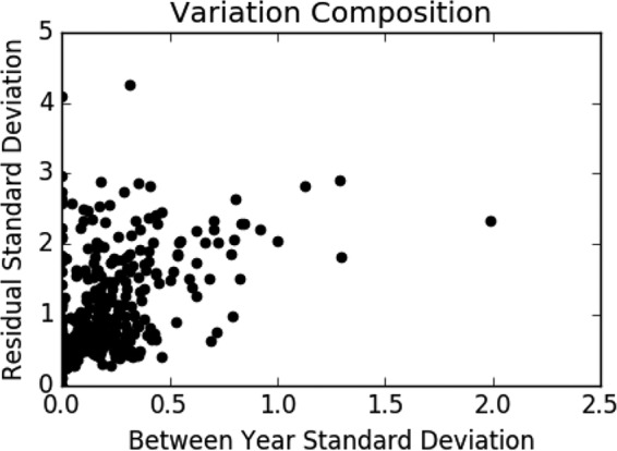
Variation composition. Scatterplot of between-year standard deviations versus residual standard deviations across all bacterium, drug, and stage combinations.

Power analysis.

As the first step of the power analysis, we determined that across all bacterium, drug, and stage combinations, the standard deviations of the log₂ MIC values decreased sharply from 0, with most values below 0.6 and almost all values below 1 (Fig. 8). As a result, power curves were plotted for standard deviations of 0.6 and 1. These curves indicate that at a standard deviation of 0.6 it would be possible to detect a 1 log₂ MIC change in 5 years, and at a standard deviation of 1 a 1.5 log₂ MIC change could be detected in 7 years.

FIG 8.

Power analysis for testing changes in mean log₂ MIC. (A) Distribution of empirical standard deviations across all bacterium, drug, and stage combinations. (B) Calculation of power assuming a standard deviation of 0.6. (C) Calculation of power assuming a standard deviation of 1. (D) Power of a test comparing 9 years before a policy change with 5 years after the change as a function of the number of isolates sampled each year. Dashed lines indicate a power of 0.8, the standard minimum power desired for a hypothesis test.

In analyzing the power of the proportion test, it was determined that the vast majority of average resistance proportions across all bacterium, drug, and stage combinations were below 0.25, with most being below 0.5, and the majority of overdispersion factors were below 2 (Fig. 9). Assuming an overdispersion of 2, in 6 years it would be possible to detect a 6% decrease in resistance if initial resistance was 25%, and it would be possible to detect an 8% decrease in 5 years if the initial resistance was increased to 50%.

FIG 9.

Power analysis for testing changes in percent resistance. (A) Distribution of empirical percent resistance across all bacterium, drug, and stage combinations. (B) Distribution of empirical overdispersion. (C) Plot of overdispersion versus sample size. (D) Calculation of power assuming an initial resistance of 25% and an overdispersion of 2. (E) Calculation of power assuming an initial resistance of 50% and an overdispersion of 2. Dashed lines indicate a power of 0.8, the standard minimum power desired for a hypothesis test.

The number of isolates sampled each year plays an important role in the power. Power increases dramatically between 1 and 100 isolates per year. It increases slowly between 100 and 500 isolates. Beyond 500 isolates the power sharply plateaus.

The above-described estimates assume that only one hypothesis test is being carried out, but in practice it would be necessary to perform one test for each bacterium-drug combination. In practice, results would need to be adjusted to account for multiple testing to protect against false positives.

Analyzing the effects of a change in enrofloxacin policy.

The exploratory analysis of the trend in C. jejuni resistance to ciprofloxacin shows that since the policy change in 2005, both mean log₂ MIC and percent resistance have remained essentially constant, if not slightly increasing, at both slaughter and retail (Fig. 10). Both generalized linear models also confirm this fact(Table 4). The t test of the difference in mean log₂ MIC before and after the policy change is not significant at retail (effect, 0.028; P = 0.9) or slaughter (effect, 0.44; P = 0.13). Removing approval for enrofloxacin in poultry did not decrease resistance to fluoroquinolones.

FIG 10.

Exploratory assessment of the 2005 tightening of enrofloxacin policy on Campylobacter jejuni resistance to ciprofloxacin. (A) Boxplots of log₂ MIC values. The dashed line indicates the breakpoint between resistant and susceptible isolates. (B) Line graph of percentage of isolates with MIC values above the resistance breakpoint. Sizes of points are proportional to the number of observations in the given year and stage. Data from 2002 to 2003 are included in this analysis, as it is an assessment of a 2005 policy change. Ciprofloxacin is studied because it is the metabolic product of enrofloxacin. Sample sizes ranged from 78 to 1,348.

TABLE 4.

Generalized linear modeling assessment of the 2005 tightening of enrofloxacin policy on Campylobacter jejuni resistance to ciprofloxacin

Coefficient	C. jejuni-ciprofloxacina
	Logistic	Linear model
α	−1.64*	−1.68*
β2003	−0.20	−0.41*
β2004	0.06	−0.56*
β2005	−0.17	−0.55*
β2006	−0.23	−0.62*
β2007	0.12	−0.26
β2008	0.09	−0.26
β2009	0.28	0.13
β2010	0.36*	0.05
β2011	0.24	0.06
β2012	0.21	0.00
βslaughter	0.14*	−0.44*

^aAn asterisk indicates significance at an α value of 0.05.

DISCUSSION

Antimicrobial resistance is a growing threat with serious implications not only for human and veterinary health but also the food supply, animal agriculture, and the economy. To counteract this threat, the FDA has proposed tightening restrictions on the use of antimicrobials. However, this change will undoubtedly have consequences for food production and pricing. With this in mind, it is essential to understand historical baseline resistance trends and to ensure it will be possible to assess the effects of the policy change on future levels of resistance.

The exploratory analysis undertaken here demonstrates that over the past decade, the percent resistance and mean log₂ MIC at both slaughter and retail have fluctuated up and down in a bacterium-drug-specific manner. The logistic and linear models confirm this observation, as both year and stage coefficients were significant in likelihood ratio tests. While logistic and linear models revealed the same overall trends, each model provides a distinctly useful view of AMR. Logistic regression provides a straightforward characterization of situations where there is a known epidemiological cutoff or clinical breakpoint between resistance and susceptibility. Logistic regression, however, is highly sensitive to the choice of breakpoint, making it opaque to interpretation when the resistance threshold is difficult to determine (20). In this case, linear regression of log₂ MIC provides a more straightforward characterization of resistance patterns. Additionally, because linear regression explains the mean resistance level, in general it can provide a more holistic view of AMR.

Mixed-effect models show that there are different levels of variation between and within years. Surprisingly, however, there is more variation within years than between years, and accounting for state does little to resolve this variation. This indicates that most of the AMR variation is due to the structure of resistance in the population.

Our analysis showed that by performing a hypothesis test comparing the level of resistance before and after a change, it is possible to detect a change in resistance level as small as 1 log₂ MIC in 5 years or a 6% change in resistance in as little as 6 years. Moreover, the current level of data collection of 200 isolates per year provides more than sufficient power and could in fact be reduced to 100 samples per year without significant reduction in power. Although it might be interesting to test the change in slope of the trend line before and after a policy change, our exploratory analysis showed that resistance patterns do not often have clear trends, so we chose to focus on a comparison test of resistance levels. Even though it would take 6 years to detect a change in AMR after the new level had been reached, which may itself take several years, this is a fairly short period of time on a policy-making scale. As a result, even though it may be difficult to predict the outcome of the current change in FDA policy, it will not be difficult to assess changes in AMR. An implicit assumption of the proposed approach is that changes in the AMR levels after policy implementation can be attributable largely to the policy. A combined analysis of the antimicrobial use and resistance would provide a greater level of evidence (21). However, in the United States, antimicrobial use data are limited to sales of active compounds aggregated by drug class intended for use in all food-producing animals since 2009 (22).

Analyzing the change in resistance before and after implementation of enrofloxacin policy reveals the complexities of managing and evaluating AMR. To the extent that there was a trend, AMR increased following the policy change, but this was not significant even for log₂ MIC values, which provide a more sensitive test. Previous studies aiming to evaluate the enrofloxacin ban reported unchanged resistance levels for ciprofloxacin in Campylobacter isolates recovered from chicken and chicken carcasses (23, 24). These previous surveys sampled a small number of isolates during short periods of time (2004 to 2006) and narrow geographical locations. Based on our analysis, AMR changes during short time spans (e.g., 2 years) are unlikely to show changes on AMR levels even if the policy was effective. A more comprehensive study analyzed changes to the proportion of isolates resistant to ciprofloxacin for Campylobacter in the NARMS retail meat samples from 2002 to 2007 and found no changes (25).

REFERENCES

- 1.Oliver SP, Murinda SE, Jayarao BM. 2011. Impact of antibiotic use in adult dairy cows on antimicrobial resistance of veterinary and human pathogens: a comprehensive review. Foodborne Pathog Dis 8:337–355. doi: 10.1089/fpd.2010.0730. [DOI] [PubMed] [Google Scholar]
- 2.Marshall BM, Levy SB. 2011. Food animals and antimicrobials: impacts on human health. Clin Microbiol Rev 24:718–733. doi: 10.1128/CMR.00002-11. [DOI] [PMC free article] [PubMed] [Google Scholar]
- 3.World Health Organization. 2014. Global action plan on antimicrobial resistance. World Health Organization, Geneva, Switzerland. [Google Scholar]
- 4.The White House. 2015. National action plan for combating antibiotic-resistant bacteria. The White House, Washington, DC. [Google Scholar]
- 5.FDA. 2012. Guidance for industry #209: the judicious use of medically important antimicrobial drugs in food-producing animals. U.S. Food and Drug Administration, Silver Spring, MD. [Google Scholar]
- 6.FDA. 2013. Guidance for industry number 213: new antimicrobial drugs and new animal drug combination products administered in or on medicated feed for drinking water of food-producing animals: recommendations for drug sponsors for voluntarily aligning product use conditions with GFI #209. U.S. Food and Drug Administration, Silver Spring, MD. [Google Scholar]
- 7.FDA. 2015. NARMS now: integrated data. U.S. Food and Drug Administration, Silver Spring, MD. [Google Scholar]
- 8.FDA. 2015. NARMS methods. U.S. Food and Drug Administration, Silver Spring, MD. [Google Scholar]
- 9.Martínez JL, Coque TM, Baquero F. 2015. What is a resistance gene? Ranking risk in resistomes. Nat Rev Microbiol 13:116–123. doi: 10.1038/nrmicro3399. [DOI] [PubMed] [Google Scholar]
- 10.Naggara O, Raymond J, Guilbert F, Roy D, Weill A, Altman DG. 2011. Analysis by categorizing or dichotomizing continuous variables is inadvisable: an example from the natural history of unruptured aneurysms. Am J Neuroradiol 32:437–440. doi: 10.3174/ajnr.A2425. [DOI] [PMC free article] [PubMed] [Google Scholar]
- 11.Fedorov V, Mannino F, Zhang R. 2009. Consequences of dichotomization. Pharm Stat 8:50–61. doi: 10.1002/pst.331. [DOI] [PubMed] [Google Scholar]
- 12.Hombach M, Mouttet B, Bloemberg GV. 2013. Consequences of revised CLSI and EUCAST guidelines for antibiotic susceptibility patterns of ESBL- and AmpC beta-lactamase-producing clinical Enterobacteriaceae isolates. J Antimicrob Chemother 68:2092–2098. doi: 10.1093/jac/dkt136. [DOI] [PubMed] [Google Scholar]
- 13.Hamada Y, Sutherland CA, Nicolau DP. 2015. Impact of revised cefepime CLSI breakpoints on Escherichia coli and Klebsiella pneumoniae susceptibility and potential impact if applied to Pseudomonas aeruginosa. J Clin Microbiol 53:1712–1714. doi: 10.1128/JCM.03652-14. [DOI] [PMC free article] [PubMed] [Google Scholar]
- 14.Lienau JA, Ellerbroek L, Klein G. 2007. Tracing flock-related Campylobacter clones from broiler farms through slaughter to retail products by pulsed-field gel electrophoresis. J Food Prot 70:536–542. [DOI] [PubMed] [Google Scholar]
- 15.Nógrády N, Kardos G, Bistyák A, Turcsányi I, Mészáros J, Galántai Z, Juhász Á, Samu P, Kaszanyitzky JÉ, Pászti J, Kiss I. 2008. Prevalence and characterization of Salmonella infantis isolates originating from different points of the broiler chicken–human food chain in Hungary. Int J Food Microbiol 127:162–167. doi: 10.1016/j.ijfoodmicro.2008.07.005. [DOI] [PubMed] [Google Scholar]
- 16.Wagner BA, Salman MD, Dargatz DA, Morley PS, Wittum TE, Keefe TJ. 2003. Factor analysis of minimum-inhibitory concentrations for Escherichia coli isolated from feedlot cattle to model relationships among antimicrobial-resistance outcomes. Prev Vet Med 57:127–139. doi: 10.1016/S0167-5877(02)00232-5. [DOI] [PubMed] [Google Scholar]
- 17.USDA. 2014. NARMS–National Antimicrobial Resistance Monitoring System Animal Isolates. U.S. Department of Agriculture, Washington, DC. [Google Scholar]
- 18.FDA. 2003. Guidance for industry #152: evaluating the safety of antimicrobial new animal drugs with regard to their microbiological effects on bacteria of human health concern. U.S. Food and Drug Administration, Silver Spring, MD. [Google Scholar]
- 19.SAS Institute Inc. 2004. SAS/STAT 9.1 user's guide, p 3409–3592. SAS Institute Inc., Cary, NC. [Google Scholar]
- 20.Jaspers S, Aerts M, Verbeke G, Beloeil PA. 2014. Estimation of the wild-type minimum inhibitory concentration value distribution. Stat Med 33:289–303. doi: 10.1002/sim.5939. [DOI] [PubMed] [Google Scholar]
- 21.EFSA. 2006. ECDC/EFSA/EMA first joint report on the integrated analysis of the consumption of antimicrobial agents and occurrence of antimicrobial resistance in bacteria from humans and food-producing animals. European Food Safety Authority, Parma, Italy. [Google Scholar]
- 22.FDA. 2013. Animal drug user fee act. U.S. Food and Drug Administration, Silver Spring, MD. [Google Scholar]
- 23.Nannapaneni R, Hanning I, Wiggins KC, Story RP, Ricke SC, Johnson MG. 2009. Ciprofloxacin-resistant Campylobacter persists in raw retail chicken after the fluoroquinolone ban. Food Addit Contam Part A Chem Anal Control Expo Risk Assess 26:1348–1353. doi: 10.1080/02652030903013294. [DOI] [PubMed] [Google Scholar]
- 24.Price LB, Leila GL, Vailes R, Silbergeld E. 2007. The persistence of fluoroquinolone-resistant Campylobacter in poultry production. Environ Health Perspect 115:1035–1039. doi: 10.1289/ehp.10050. [DOI] [PMC free article] [PubMed] [Google Scholar]
- 25.Zhao S, Young SR, Tong E, Abbott JW, Womack N, Friedman SL, McDermott PF. 2010. Antimicrobial resistance of Campylobacter isolates from retail meat in the United States between 2002 and 2007. Appl Environ Microbiol 76:7949–7956. doi: 10.1128/AEM.01297-10. [DOI] [PMC free article] [PubMed] [Google Scholar]