Semi-physical Identification and State Estimation of Energy Intake for Interventions to Manage Gestational Weight Gain

Abstract

Excessive gestational weight gain (i.e., weight gain during pregnancy) is a significant public health concern, and has been the recent focus of novel, control systems-based interventions. This paper develops a control-oriented dynamical systems model based on a first-principles energy balance model from the literature, which is evaluated against participant data from a study targeted to obese and overweight pregnant women. The results indicate significant under-reporting of energy intake among the participant population. A series of approaches based on system identification and state estimation are developed in the paper to better understand and characterize the extent of under-reporting; these range from back-calculating energy intake from a closed-form of the energy balance model, to a constrained semi-physical identification approach that estimates the extent of systematic under-reporting in the presence of noise and possibly missing data. Additionally, we describe an adaptive algorithm based on Kalman filtering to estimate energy intake in real-time. The approaches are illustrated with data from both simulated and actual intervention participants.

I. Introduction

The high prevalence of obesity and excessive gestational weight gain are major contributors to adverse pregnancy and birth outcomes [1]. In 2009, the US Institute of Medicine (IOM) revised its recommendations for total and rate of weight gain for pregnant women by different categories of pre-pregnancy body mass index (BMI) [2]. A 2014 study shows that 71% of overweight (OW; BMI ≥ 25 kg/m²) women and 61% of obese (OB; BMI ≥ 30 kg/m²) women gained weight in excess of the IOM recommendations [3]. Gestational weight gain higher than the IOM recommendations substantially increases the risk of gestational diabetes mellitus, preeclampsia, emergency cesarean delivery, and postpartum weight retention in pregnant women [3], [4]. Furthermore, infants of OW/OB mothers are more likely to be preterm, large for gestational age and have an increased risk of developing obesity from infancy to adulthood [1], [3]. Therefore, there exists a great need to develop interventions which can effectively help pregnant women maintain weight gain within IOM guidelines, and further improve maternal and infant health.

This work is motivated by the needs of an intervention, the Healthy Mom Zone study (HMZ; [5]) that is being conducted at Penn State University. The HMZ study aims to develop and validate an individually-tailored intensively adaptive intervention involving healthy eating, physical activity, goal-setting, self-monitoring, and other cognitive behavioral strategies to effectively manage weight gain in pregnancy. In prior work [6], a comprehensive dynamical systems model for a behavioral intervention to control gestational weight gain was proposed. This model relies on the integration of a first-principles energy balance (EB) model developed by Thomas et al. [7] with a dynamical behavioral model based on the Theory of Planned Behavior.

In this paper, we re-evaluate the EB model in the context of the initial HMZ pilot study, and develop some extensions. Specifically, we reformulate the original EB model as a parsimonious dynamical system with one output (maternal weight) and two inputs (energy intake (EI) and physical activity). This reformulated EB model is amenable to control analysis, and compensates for the limitations of the original EB model that did not explicitly include the impact of changes in physical activity on weight gain (or loss).

The effectiveness of the reformulated EB model is evaluated against the measured data of OW/OB pregnant women from the pilot study. Underreporting of EI is a commonly observed problem in weight interventions using self-reported data [8]. To understand the extent of underreporting, estimates of the true EI for a participant are back-calculated from a discretized, closed-form version of the reformulated EB model and compared with the self-reported EI. A semi-physical identification approach based on quadratic programming (QP) that estimates the extent of systematic underreporting in a participant is also developed. This method is better able to cope with missing data, and also provides a statistical confidence interval of the estimates. Finally, we develop a recursive method based on Kalman filtering that could be used to sequentially estimate EI in real-time.

The paper is organized as follows. Section II presents an overview of the reformulated dynamical EB model based on the Thomas et al. EB model [7]. Section III evaluates the prediction of gestational weight gain from the reformulated EB model using participant data, ultimately leading to a semi-physical estimation approach to estimating the true EI from the self-reported EI. In Section IV, the adaptive algorithm based on Kalman filtering to estimate EI in real-time is developed and tested against the data from actual participants. Section V gives a summary of our conclusions.

II. Modeling overview

A. Review of Thomas et al. Energy Balance Model

The EB model to predict gestational weight gain (GWG) based on gestational energy intake (EI) and energy expenditure (EE) relies on the principle of energy conservation, which can be expressed as,

$$\mathit{\text{ES}}\left(t\right)=(1-g)\mathit{\text{EI}}\left(t\right)-\mathit{\text{EE}}\left(t\right)$$ (1)

where ES(t) is the energy stored at time t; the parameter g = 0.03 is the nutrient partitioning constant. This two-compartment model describes the maternal body weight (W) by the sum of fat free mass (FFM) and fat mass (FM).

$$W\left(t\right)=\mathit{\text{FFM}}\left(t\right)+FM\left(t\right)$$ (2)

Expansion of the ES term into the sum of the instantaneous weight change of the two components of FM and FFM, multiplied by their respective energy densities λ_FM and λ_FFM, leads to the final differential equation of the EB model as follows,

$${\mathrm{\lambda }}_{\mathit{\text{FFM}}}\frac{\mathit{\text{dFFM}}\left(t\right)}{dt}+{\mathrm{\lambda }}_{FM}\frac{\mathit{dFM}\left(t\right)}{dt}=\left(1-g\right)EI(t)-EE(t)$$ (3)

where λ_FM = 9500 kcal/kg, λ_FFM = 771 kcal/kg.

B. Reformulated Energy Balance Model

As noted in [9], the Thomas et al. model estimates the EE as a monolithic quantity. This means that the model does not break down into the different elements of EE. EE is commonly divided into three components: PA, resting metabolic rate (RMR), and thermic effect of food (TEF) [10]. As a result, the EE value cannot be adjusted if an individual has higher level of PA due to interventions, for example. Here, modifications are made.

TEF is usually expressed as a percentage of EI, ranging from 4.0% to 17.1% due to different diets [11]. Regardless of intake nutrients, we assume it to be approximately 7% of daily EI as measured in [12]. In this initial analysis, we will consider RMR constant during gestation, which leads to,

$$EE\left(t\right)=PA\left(t\right)+\mathit{RMR}+r_{\mathit{TEF}}EI\left(t\right)$$ (4)

where r_TEF = 0.07. Substituting (4) and (2) into (3) gives,

$$\begin{array}{l}{\mathrm{\lambda }}_{\mathit{\text{FFM}}}\frac{d\mathit{\text{FFM}}\left(t\right)}{dt}+{\mathrm{\lambda }}_{FM}\frac{d\left(W\left(t\right)-\mathit{\text{FFM}}\left(t\right)\right)}{dt}\\ =\left(1-g-r_{\mathit{TEF}}\right)EI\left(t\right)-PA\left(t\right)-\mathit{RMR}\end{array}$$ (5)

Instead of keeping two differential terms in (5), FFM can be manipulated to relate to W so that the derivative is only with respect to W and the equations become much easier to solve. To begin with, FFM can be considered to be the sum of total body water (TBW), total body protein (TBP), and mass that stays constant during gestation (written as CM); this latter quantity includes bone mass. This leads to,

$$\mathit{\text{FFM}}\left(t\right)=\mathit{TBW}\left(t\right)+\mathit{TBP}\left(t\right)+CM$$ (6)

where CM = FFM (0) − TBW (0) − TBP (0).

TBW and TBP are linear functions of simultaneously measured W based on a participant’s BMI (see Table I), which can be expressed in a generalized form as,

$$\mathit{TBW}\left(t\right)=a_{W}W\left(t\right)+b_W$$ (7a)

$$\mathit{TBP}\left(t\right)=a_{P}W\left(t\right)+b_P$$ (7b)

where a_W, b_W, a_P, b_P are the coefficients of the corresponding functions. Substituting (7) into (6) leads to,

$$\mathit{\text{FFM}}\left(t\right)=\left(a_W+a_P\right)W\left(t\right)+\left(b_W+b_P+CM\right)$$ (8)

which if substituted into (5) gives the differential equation expressed in terms of the derivative of W as,

$$\frac{dW(t)}{dt}=K_{1}EI(t)+K_{2}PA(t)+K_2\mathit{RMR}$$ (9)

where

$$K_1=\frac{1-g-r_{\mathit{TEF}}}{\left(a_W+a_P\right){\mathrm{\lambda }}_{\mathit{\text{FFM}}}+\left(1-a_W-a_P\right){\mathrm{\lambda }}_{FM}}$$ (10a)

$$K_2=\frac{-1}{\left(a_W+a_P\right){\mathrm{\lambda }}_{\mathit{\text{FFM}}}+\left(1-a_W-a_P\right){\mathrm{\lambda }}_{FM}}$$ (10b)

K₁ and K₂ are both in kg/kcal/day. Equation (9) forms the basis of the work presented in this paper, from which we are able to predict the system output W using the explicitly measurable inputs EI and PA. When written in deviation variables and using Laplace transforms, (9) gives,

$$\mathrm{\Delta }W\left(s\right)=\frac{K_1}{s}\mathrm{\Delta }EI\left(s\right)+\frac{K_2}{s}\mathrm{\Delta }PA\left(s\right)$$ (11)

As seen here, the reformulated EB model for GWG can be represented in terms of a simple sum of integrators, with K₁ and K₂ (the system gain coefficients) corresponding to each of the two inputs. Table II shows the values of K₁ and K₂ categorized by BMI.

TABLE I.

Tabulation of linear functions of total body water (TBW) and total body protein (TBP) with respect to maternal weight (W). TBP and W are expressed in kg, TBW in liters.

BMI Category (kg/m2)	Weight Range (kg)	TBW Function	TBP Function
Low BMI (≤ 19.8)	W ≤ 52	0.489W + 3.875	−0.04762W +9.28
	52 < W ≤ 57.7		0.105263W + 1.33
	W > 57.7		0.075472W + 3.05
Normal BMI (19.8–26)	W ≤ 60.2	0.4836W + 2.853	−0.667W + 47.533
	60.2 < W ≤ 65.1		0.0204W + 6.17
	W > 65.1		0.0724W + 3.05
High BMI (≥ 26)	W ≤ 81.8	0.503W + 4.885	−0.03226W + 10.4387
	81.8 < W ≤ 85.8		0.1W − 0.38
	W > 85.8		0.098765W + 0.27407

TABLE II.

System gain parameters for energy intake (K₁) and physical activity (K₂) for low, normal and high BMI.

BMI Category (kg/m2)	Weight Range (kg)	Gain K1 (kg/kcal/day)	Gain K2 (kg/kcal/day)
Low BMI (≤ 19.8)	W ≤ 52	1.59 × 10−4	−1.77 × 10−4
	52 < W ≤ 57.7	2.09 × 10−4	−2.32 × 10−4
	W > 57.7	1.97 × 10−4	−2.19 × 10−4
Normal BMI (19.8–26)	W ≤ 60.2	0.81 × 10−4	−0.90 × 10−4
	60.2 < W ≤ 65.1	1.76 × 10−4	−1.96 × 10−4
	W > 65.1	1.94 × 10−4	−2.15 × 10−4
High BMI (≥ 26)	W ≤ 81.8	1.67 × 10−4	−1.85 × 10−4
	81.8 < W ≤ 85.8	2.12 × 10−4	−2.36 × 10−4
	W > 85.8	2.12 × 10−4	−2.35 × 10−4

III. Semi-physical identification for batch data

A. EI Estimation Using Closed-Form EB model

Using the EB model in (9), simulations are run with the measured data from the pilot study. In the pilot study, EI, PA and W of 22 OW/OB pregnant women were measured for 6 weeks. Participant EI is obtained from self-reports using a dietary intake phone app (MyFitnessPal). The measurements of PA are obtained using a wrist-worn commercial monitor (Jawbone UP). Because EI measurements are not obtained daily, there will be missing data. For any missing data in the system variables, linear interpolation is used to impute the missing days so that simulations can be performed. RMR was not measured in the pilot study, but will be measured and objectively assessed over pregnancy in the full trial. In this paper, we consider RMR constant during gestation, defined at baseline for each participant. The baseline RMR is calculated using the quadratic regression formula proposed by Thomas et al. [13], which fits Butte et al.’s data [14] as shown below:

$$\mathit{RMR}=0.1976W_b^2-13.424W_b+1457.6$$ (12)

W_b is the maternal weight at baseline of the intervention, expressed in kg.

Simulation results of the selected two participants are presented in Fig. 1, where it can be seen that the predicted W using the self-reported EI (drawn in blue) lies below the measured W (drawn in black), with discrepancies accumulating along the 6 weeks. Similar biases in weight prediction are also observed for most other participants. While these can be explained in part from the imputation of missing data, the more significant explanation for this variance is as a result of under-reported EI. Literature consistently demonstrates that a large number of subjects under-report EI [8], [15]. A 2012 study found that up to 45% of pregnant women could potentially be under-reporting their daily EI, with having a BMI in the overweight/obese category being the main predictor of EI under-reporting [16].

Fig. 1.

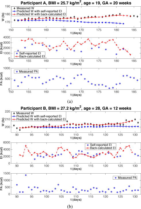
Simulations of the reformulated EB model using self-reported and back-calculated EI from two representative intervention participants. BMI: body mass index; GA: gestational age at baseline.

To test this hypothesis, we back-calculate EI using the reformulated EB model, the measurements of W, PA, and the values of RMR, τTEF, K₁ and K₂ from Table II. Numerically approximating the derivative term in (9) using the 2nd order centered difference formula leads to the expression of the estimated EI (EI_est) as shown below,

$$\begin{array}{c}E{I}_{\mathit{est}}(k)=\frac{-W(k+2)+8W(k+1)-8W\left(k-1\right)+W\left(k-2\right)}{12T{K}_1}\\ -\frac{K_2}{K_1}\left(PA\right(k)+\mathit{RMR})\end{array}$$ (13)

The variables are indexed by k with k = 1, 2, …, N corresponding to day 1 to day N. T is the sampling time, in this case, T = 1 day. The noise in W is small relative to the total W; however the extent of this noise can significantly affect the numerical calculation of the rate of weight gain per day. Consequently, a five-day moving average filter is used to preprocess (i.e., smooth) the measured W before a “true” daily EI is estimated from (13). As shown in Fig. 1, the backtracked EI (drawn in red) is generally higher than the reported EI measurements (drawn in blue). The difference between the back-calculated EI and the self-reported EI is quantified using the mean error (ME) and its standard deviation (SD). The ME ± SD of the EI estimate for participant A is 787 ± 617 kcal; the ME±SD for participant B is 353 ± 1025 kcal. It is also noticed that the predicted W using the back-calculated EI follows closely with the measured W, which also proves the accuracy of the EI back-calculation from this method.

B. Constrained Semi-Physical Identification Approach

To further understand the portion of EI that is systematically under-reported, we propose a simple linear formula to describe the relationship between true EI (EI_true) and reported EI (EI_rept); this follows according to (14).

$$E{I}_{\mathit{true}}\left(k\right)=\alpha E{I}_{\mathit{rept}}\left(k\right)+\gamma$$ (14)

The random portion of the EI report is treated as a noise signal added to EI_rept,

$$E{I}_{\mathit{rept}}^{\prime }\left(k\right)=E{I}_{\mathit{rept}}\left(k\right)+n_{EI}\left(k\right)$$ (15)

where $E{I}_{\mathit{rept}}^{\prime }$ is the self-reported EI measurement signal. In order to relate EI_rept in (14) to the EB model, the EB model is discretized. Using a 1st order forward difference approximation to discretize (9) leads to,

$$\mathit{GWG}(k+1)=K_{1}E{I}_{\mathit{true}}\left(k\right)+K_{2}PA\left(k\right)+K_2\mathit{RMR}$$ (16)

where (for T = 1 day)

$$\mathit{GWG}\left(k+1\right)=W\left(k+1\right)-W\left(k\right)\cong \frac{dW\left(t\right)}{dt}$$ (17)

Combining (14) with (16) leads to,

$$\mathit{GWG}\left(k+1\right)={\theta }_{1}E{I}_{\mathit{rept}}\left(k\right)+{\theta }_{2}PA\left(k\right)+{\theta }_3$$ (18)

where θ₁ = K₁α, θ₂ = K₂, θ₃ = K₁γ + K₂RMR. Equation (18) directly relates the reported EI to the output of EB model.

In real life conditions, the measurement of GWG is corrupted by noise, which is expressed as,

$$GW{G}_{\mathit{meas}}\left(k\right)=\mathit{GWG}\left(k\right)+n_{\mathit{GWG}}\left(k\right)$$ (19)

GWG_meas is the measurement of GWG, and n_GWG is the random measurement noise. A regression problem can be formulated based on (18) as shown below,

$$\stackrel{Z}{\overbrace{\left[\begin{array}{c}GW{G}_{\mathit{meas}}\left(k_1+1\right)\\ GW{G}_{\mathit{meas}}\left(k_2+1\right)\\ ⋮\\ GW{G}_{\mathit{meas}}\left(k_N+1\right)\end{array}\right]}}=\begin{array}{cc}\stackrel{R}{\overbrace{\left[\begin{array}{ccc}E{I^{\prime }}_{\mathit{rept}}\left(k_1\right)& PA\left(k_1\right)& 1\\ E{I^{\prime }}_{\mathit{rept}}\left(k_2\right)& PA\left(k_2\right)& 1\\ ⋮& ⋮& ⋮\\ E{I^{\prime }}_{\mathit{rept}}\left(k_N\right)& PA\left(k_N\right)& 1\end{array}\right]}}& \stackrel{\theta }{\overbrace{\left[\begin{array}{c}{\theta }_1\\ {\theta }_2\\ {\theta }_3\end{array}\right]}}\end{array}$$ (20)

where Z ∈ ℝ^N is the vector of output measurements, R ∈ ℝ^{N × 3} is the regressor that stores input measurements, θ ∈ ℝ³ is the parameter vector that needs to be estimated, and k₁, k₂,…, k_N are the days at which the measurements of all three variables (inputs EI, PA; output GWG) are available. The data flow for this liner regression model is illustrated in the block diagram in Fig. 2.

Fig. 2.

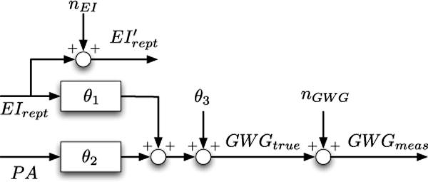
Block diagram of the linear regression model.

The regression formula per (20) uses only available data and eliminates the need for imputation. To identify the parameter vector θ, a least squares cost function is considered:

$$J\left(k\right)=\underset{\widehat{\theta }}{\text{min}}\left\{\frac{1}{2}{\left[Z-R\widehat{\theta }\right]}^2\right\}$$ (21)

Constraints for each coefficient can be imposed based on prior knowledge of the sign of the system gains K₁ > 0, K₂ < 0 and the coefficient α > 0. The solution to (21) is accomplished based on quadratic programming (QP). The problem statement is formulated as follows,

$$\begin{array}{cc}\underset{\theta }{\text{min}}& \{\frac{1}{2}{\theta }^{T}H\theta +f^T\theta \}\\ s.t.& G\theta <\mathbf{0}\end{array}$$ (22)

where H = 2R^T R, f = (−2Z^T R)^T, $G=\left[\begin{array}{ccc}-1& 0& 0\\ 0& 1& 0\\ 0& 0& 0\end{array}\right]$.

The solution to the QP problem in (22) gives the estimates of θ, from which α and γ, the coefficients used to model the under-reported EI in (14) can be calculated. This leads to the estimate of EI from the self-reported $E{I}_{\mathit{rept}}^{\prime }$ as shown below,

$$E{I}_{\mathit{est}}\left(k\right)=\widehat{\alpha }E{I}_{\mathit{rept}}^{\prime }\left(k\right)+\widehat{\mathrm{\gamma }}$$ (23)

where “hat” denotes the estimate. The standard errors of the estimated coefficients for this linear regression model are calculated by bootstrapping the residuals between the estimated and measured GWG.

This estimation method is evaluated in simulations using a hypothetical participant first. The results are shown in Fig. 3. For this simulated participant, we fix the values of α, γ, EI_rept, PA, and the statistics of the random noises n_GWG, n_EI, from which the θ_1–3, GWG, GWG_meas, $E{I}_{\mathit{rept}}^{\prime }$ and EI_true for that participant can be calculated to form the regression model. From the model, the true EI can be estimated using the QP algorithm and compared with the assumed values. It can be seen from the results in Fig. 3 that EI_est are on average higher than the self-reported EI, but remain close to the true EI values.

Fig. 3.

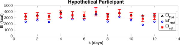
A hypothetical case for EI estimation using the semiphysical identification approach. Here, n_EI ~ N(0, 400²), n_GWG ~ N(0, 0.1²); α = 1.1, γ = 400. Error bars represent the 95% confidence interval calculated using bootstrp in MATLAB®.

In Fig. 4, the results calculated from two intervention participants are presented. As with the back-calculation examples from Section III.A, a five-day moving average filter is used for GWG_meas prior to applying the semi-physical estimation procedure. EI_est for participant A is consistently higher than the self-reported EI by an ME ± SD of 900 ± 355 kcal. Participant B, meanwhile, has an ME ± SD of 528 ± 519 kcal.

Fig. 4.

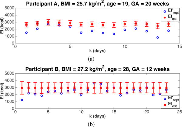
The results of estimating the true EI from self-reported EI for two intervention participants using the proposed semi-physical identification approach. Error bars represent the 95% confidence interval.

IV. Kalman Filtering Approach for EI Estimation

In this section, we develop a recursive method based on Kalman filtering (KF) to sequentially estimate EI in real-time. In this method, the variable we aim to estimate, i.e., EI in this application, is viewed as the “state” of a system. We treat this “state” invariant in time but affected by noise, which leads to the state equation expressed as,

$$EI\left(k+1\right)=EI\left(k\right)+w\left(k+1\right)$$ (24)

where the random variable w(k) represents the process noise. The discretized EB model equation in (16) is used as the measurement equation but with PA and RMR as system inputs. If the state of this system is denoted by x = [EI], the input by u = [PA, RMR]^T and the output y = [GWG] respectively, we can write the dynamics of this discrete system by coupling (24) with (16) as,

$$x\left(k+1\right)=Ax\left(k\right)+Bu\left(k+1\right)+w\left(k+1\right)$$ (25a)

$$y\left(k+1\right)=Cx\left(k+1\right)+Du\left(k+1\right)+v\left(k+1\right)$$ (25b)

where A = I, B = 0, C = [K₁], and D = [K₂, K₂]. The random variable v(k) represents the measurement noise.

In the described system equations, both the model prediction and the measurement are subject to noise. We assume these two noise terms, w(k) and v(k) are i.i.d. over time, zero mean Gaussian with variance ϑ² and σ² respectively, that is, w(k) ~ N(0, ϑ²) and v(k) ~ N(0, σ²) for all k.

The recursive Kalman filtering algorithm is described in detail below, where “hat” denotes the estimate, P the error covariance, and K the Kalman gain.

1. Initialize:

   Set $\widehat{x}\left(0|0\right)=E{I}_0$, P(0|0) = I. EI₀ is the initial value of EI, calculated using the quadratic regression formula [17] as shown below,

   $$E{I}_0=E{E}_0=0.278W_b^2+9.2893W_b+1528.90$$ (26)
2. Predict:

   $$\begin{array}{l}\widehat{x}\left(k+1|k\right)=A\widehat{x}\left(k|k\right)+Bu\left(k+1\right);\\ P\left(k+1|k\right)=AP\left(k|k\right)A^{\prime }+Q\left(k+1\right);\end{array}$$
3. Update:

   $$\begin{array}{l}K\left(k+1\right)=P\left(k+1|k\right)C^{\prime }{\left[CP\left(k+1|k\right)C^{\prime }+R\left(k+1\right)\right]}^{-1};\\ \widehat{x}\left(k+1|k+1\right)=\widehat{x}\left(k+1|k\right)+K\left(k+1\right)\left[y\left(k+1\right)-\widehat{y}\left(k+1|k\right)\right];\\ P\left(k+1|k+1\right)=\left(I-K\left(k+1\right)C\right)P\left(k+1|k\right).\end{array}$$

   where Q(k + 1) is the covariance for process noise w(k + 1) with Q(k + 1) = ϑ²; R(k + 1) is the covariance for measurement noise v(k + 1) with R(k + 1) = σ².

For performance evaluation, we use the Root Mean Square Error (RMSE) as the metric, which is defined as,

$$\mathit{RMSE}=\sqrt{\frac{1}{T_{\mathit{span}}}{\displaystyle \sum _{k=1}^{T_{\mathit{span}}}{\left(\widehat{y}\left(k\right)-y\left(k\right)\right)}^2}}$$ (27)

T_span = 1 when calculating the running RMSE.

To test the performance of the algorithm, we create the input data, output data, as well as noise with known statistics for a hypothetical participant, similar to what was done in Section III. The simulation result using the hypothetical data is presented in Fig. 5, where Q = ϑ² = 10000, R = σ² = 0.1. It can be seen that the EI “adapts” from a given initial value and keeps tracking the true EI closely despite the presence of noise during the KF algorithm. The algorithm also produces better weight gain predictions than the noise corrupted measurements.

Fig. 5.

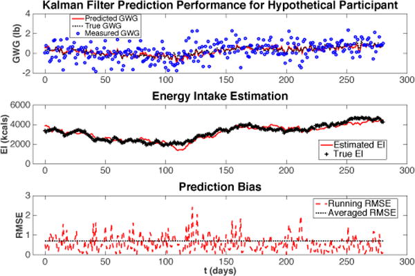
The performance of the KF algorithm illustrated using a hypothetical participant. The RMSE stands for Root Mean Square Error.

The results of the two simulations using actual participant data are presented in Fig. 6, where Q = ϑ² = 100000, R = σ² = 0.2 are set for both participants. It can be seen that the estimates of the true EI using this algorithm lie above the self-reported measures of EI, which is consistent with what we find using the two estimation approaches presented in the preceding sections. From the simulation result, the ME±SD of the EI estimate is 1111 ± 568 kcal for participant A, and 198 ± 784 kcal for participant B.

Fig. 6.

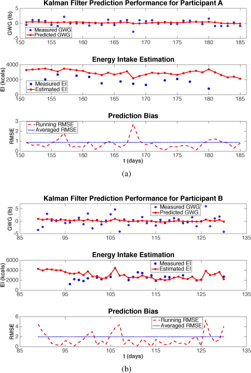
Performance of the KF algorithm evaluated using two actual intervention participants.

V. CONCLUSIONS

In this work, a control-oriented energy balance model for gestational weight gain has been developed, starting from the first-principles model of Thomas et al. [7]. The reformulated EB model can be used in the design and analysis of adaptive interventions to manage gestational weight gain, and lends itself to system identification. The model supports the development of methods for estimating underreporting of energy intake, a problem that is common in weight interventions relying on self-reports. An initial estimate of underreporting of EI is generated by back-calculating EI from measurements of W and PA using the discretized EB model equation. This leads to the formulation of a semi-physical identification problem using batch data that can be used to estimate systematic underreporting of EI in the presence of noise and despite missing data; statistical confidence bounds generated by bootstrapping are also presented. Finally, an adaptive algorithm based on Kalman filtering for real-time estimation of EI is developed; the results obtained are observed to be comparable with those from semi-physical identification. The filtering approach can also be applied to estimate other system variables whose measurements may be missing or may be imprecise, for example, RMR. All three methods are illustrated with participant data from an on-going study. Future efforts consist of generalizing some model assumptions, as well as incorporating dynamic change in RMR during both modeling and estimation. The variation in the extent of underreporting during different gestational trimesters needs also to be studied further.

References

- 1.Galtier-Dereure F, Boegner C, Bringer J. Obesity and pregnancy: complications and cost. The American Journal of Clinical Nutrition. 2000;71(5):1242s–1248s. doi: 10.1093/ajcn/71.5.1242s. [DOI] [PubMed] [Google Scholar]
- 2.Weight Gain During Pregnancy: Reexamining The Guidelines. The National Academies Press; 2009. [PubMed] [Google Scholar]
- 3.Haugen M, et al. Associations of pre-pregnancy body mass index and gestational weight gain with pregnancy outcome and postpartum weight retention: a prospective observational cohort study. BMC Pregnancy and Childbirth. 2014;14(1):201. doi: 10.1186/1471-2393-14-201. [DOI] [PMC free article] [PubMed] [Google Scholar]
- 4.Carreno CA, et al. Excessive early gestational weight gain and risk of gestational diabetes mellitus in nulliparous women. Obstetrics and Gynecology. 2012;119(6):1227–1233. doi: 10.1097/AOG.0b013e318256cf1a. [DOI] [PMC free article] [PubMed] [Google Scholar]
- 5.Healthy Mom Zone Study. [Online; accessed: September 2015]. https://sites.psu.edu/healthymomzonestudysecure/
- 6.Dong Y, Rivera DE, Thomas DM, Navarro-Barrientos JE, Downs DS, Savage JS, Collins LM. A dynamical systems model for improving gestational weight gain behavioral interventions. Proceedings of 2012 American Control Conference (ACC) 2012:4059–4064. doi: 10.1109/acc.2012.6315424. [DOI] [PMC free article] [PubMed] [Google Scholar]
- 7.Thomas DM, Navarro-Barrientos JE, Rivera DE, Heymsfield SB, Bredlau C, Redman LM, Martin CK, Lederman SA, Collins LM, Butte NF. Dynamic energy balance model predicting gestational weight gain. The American Journal of Clinical Nutrition. 2012;95(1):115–122. doi: 10.3945/ajcn.111.024307. [DOI] [PMC free article] [PubMed] [Google Scholar]
- 8.Lichtman SW, et al. Discrepancy between self-reported and actual caloric intake and exercise in obese subjects. New England Journal of Medicine. 1992;327(27):1893–1898. doi: 10.1056/NEJM199212313272701. [DOI] [PubMed] [Google Scholar]
- 9.Sabounchi NS, Hovmand PS, Osgood ND, Dyck RF, Jungheim ES. A novel system dynamics model of female obesity and fertility. Amer Journal of Public Health. 2014;104(7):1240–1246. doi: 10.2105/AJPH.2014.301898. [DOI] [PMC free article] [PubMed] [Google Scholar]
- 10.Ravussin E, Bogardus C. A brief overview of human energy metabolism and its relationship to essential obesity. The American Journal of Clinical Nutrition. 1992;55(1):242s–245s. doi: 10.1093/ajcn/55.1.242s. [DOI] [PubMed] [Google Scholar]
- 11.Westerterp KR. Diet induced thermogenesis. Nutrition & Metabolism. 2004;1(1):5. doi: 10.1186/1743-7075-1-5. [DOI] [PMC free article] [PubMed] [Google Scholar]
- 12.Piers LS, Diggavi SN, Thangam S, Van Raaij JM, Shetty PS, Hautvast JG. Changes in energy expenditure, anthropometry, and energy intake during the course of pregnancy and lactation in well-nourished indian women. The American Journal of Clinical Nutrition. 1995;61(3):501–513. doi: 10.1093/ajcn/61.3.501. [DOI] [PubMed] [Google Scholar]
- 13.Thomas DM, Navarro-Barrientos JE, Rivera DE, Heymsfield SB, Collins LM. A dynamical fetal-maternal model of gestational weight gain. Personal Communication. 2009 Oct; [Google Scholar]
- 14.Butte NF, Wong WW, Treuth MS, Ellis KJ, Smith EOB. Energy requirements during pregnancy based on total energy expenditure and energy deposition. The American Journal of Clinical Nutrition. 2004;79(6):1078–1087. doi: 10.1093/ajcn/79.6.1078. [DOI] [PubMed] [Google Scholar]
- 15.Dhurandhar NV, et al. Energy balance measurement: when something is not better than nothing. International Journal of Obesity. 2014 [Google Scholar]
- 16.McGowan CA, McAuliffe FM. Maternal nutrient intakes and levels of energy underreporting during early pregnancy. European Journal of Clinical Nutrition. 2012;66(8):906–913. doi: 10.1038/ejcn.2012.15. [DOI] [PubMed] [Google Scholar]
- 17.Thomas DM, Martin CK, Heymsfield S, Redman LM, Schoeller DA, Levine JA. A simple model predicting individual weight change in humans. Journal of Biological Dynamics. 2011;5(6):579–599. doi: 10.1080/17513758.2010.508541. [DOI] [PMC free article] [PubMed] [Google Scholar]