Fast Inference for the Latent Space Network Model Using a Case-Control Approximate Likelihood

Abstract

Network models are widely used in social sciences and genome sciences. The latent space model proposed by (Hoff et al. 2002), and extended by (Handcock et al. 2007) to incorporate clustering, provides a visually interpretable model-based spatial representation of relational data and takes account of several intrinsic network properties. Due to the structure of the likelihood function of the latent space model, the computational cost is of order O(N²), where N is the number of nodes. This makes it infeasible for large networks. In this paper, we propose an approximation of the log likelihood function. We adopt the case-control idea from epidemiology and construct a case-control likelihood which is an unbiased estimator of the full likelihood. Replacing the full likelihood by the case-control likelihood in the MCMC estimation of the latent space model reduces the computational time from O(N²) to O(N), making it feasible for large networks. We evaluate its performance using simulated and real data. We fit the model to a large protein-protein interaction data using the case-control likelihood and use the model fitted link probabilities to identify false positive links.

1 Introduction

Networks consist of the links between members of a set of actors that are connected by a specific kind of relationship. Networks have many applications in social science, political science, and recently in genome science. Examples include friendship among students in a high school, international trade and conflicts, and protein-protein interactions. Statistical models are widely used to represent such data. Statistical network models include exponential random graph models (Frank and Strauss 1986; Wasserman and Pattison 1996), the homogeneous monadic Markov model (Frank and Strauss 1986), the stochastic blockmodel (Wang and Wong 1987), the latent class membership model (Nowicki and Snijders 2001) and the mixed membership stochastic blockmodel (Airoldi et al. 2008).

Hoff, Raftery, and Handcock (2002) proposed a stochastic model for representing network data based on the concept of “social space” (McFarland and Brown 1973). The key idea behind this model is that the observed relations are determined by the unobserved latent characteristics of the actors. These latent characteristics are represented by the actors’ unobserved latent positions in a Euclidean space. The probability of a link between two actors is determined by the distance between their latent positions and, given the latent positions of the actors, the relational ties are independent. Specifically, for a network of size N, the latent space model is as follows:

$$\text{Pr}(Y|Z,X,\mathit{\theta })=\prod _{i\ne j}P(y_{ij}|z_i,z_j,x_{ij},\mathit{\theta }),$$ (1)

where X and x_ij are observed covariates, θ are parameters and Z are latent positions, where both θ and Z are to be estimated. The probability of a link between actors i and j, Pr(y_ij|z_i, z_j, x_ij, θ), can be conveniently modeled by a logistic regression model, namely

$${\eta }_{ij}=\text{log odds}(y_{ij}=1|z_i,z_j,x_{ij},\alpha ,\beta )=\alpha +\beta \prime x_{ij}-|z_i-z_j|.$$ (2)

To complete the model specification, we assume that the z_i’s themselves are independent draws from a distribution. Hoff et al. (2002) assumed that this was a spherical multivariate normal distribution, so that

$$z_1,\cdots ,z_N\stackrel{\mathrm{i}\mathrm{i}\mathrm{d}}{~}\mathrm{M}\mathrm{V}{\mathrm{N}}_k(0,{\sigma }_z^2{I}_k),$$ (3)

where k is the dimension of the latent space. Thus the latent space network model is a hierarchical model for the y_ij, where the distribution of the y_ij depends on the z_i, and the z_i in turn have a distribution specified by ${\sigma }_z^2$.

The latent space model provides a visual and interpretable model-based spatial representation of relational data and takes account of several intrinsic network properties, including transitivity and homophily on both unobserved and observed attributes. Handcock, Raftery, and Tantrum (2007) extended the latent space model to allow clustering of the subjects in the network, beyond what would be implied by simple transitivity. Instead of assuming that the z_i come from a multivariate normal distribution, they assumed that the z_i are from a mixture of multivariate normal distributions, namely

$$z_i~\sum _{g=1}^G{\lambda }_g\mathrm{M}\mathrm{V}{\mathrm{N}}_k({\mu }_g,{\sigma }_g^2{I}_k),$$

where λ_g is the probability that an actor belongs to the gth group, λ_g ≥ 0 and ${\sum }_{g=1}^G{\lambda }_g=1$.

The log likelihood of α, β and the z_i’s for the latent space model is as follows:

$$\text{log Pr}(Y|\eta )=\sum _{i\ne j}\{{\eta }_{ij}{y}_{ij}-\text{log}(1+e^{{\eta }_{ij}})\},$$ (4)

where η_i,j = α + β′x_i,j − |z_i − z_j|. Calculation of this log likelihood involves a sum over N(N − 1) terms, which is of the order of O(N²) terms. When the relationship is undirected, the number of terms is $\left(\begin{array}{c}\hfill N\hfill \\ \hfill 2\hfill \end{array}\right)=\frac{1}{2}N(N-1)$, which is still O(N²).

In order to estimate the regression coefficients α, β, the latent positions z and their variance ${\sigma }_z^2$, it is standard to apply a Bayesian approach by constructing a Markov chain with stationary distributions equal to the posterior distribution of the parameters (Hoff et al. 2002; Handcock et al. 2007; Krivitsky et al. 2009). The algorithm proceeds with Metropolis updates for α, β and the z_i’s, generating random proposal values of these parameters from symmetric distributions centered around their current values, and then accepting these proposals with the appropriate probability. The ${\sigma }_z^2$ parameter is updated with a Gibbs step, generated by sampling a new value from the full conditional distribution:

• For each i in a random order, propose a value $z_i^{*}$ and accept with probability $\frac{p(Y|z^{*},X,\beta )\varphi (z_i^{*})}{p(Y|z,X,\beta )\varphi (z_i)}$.

• Propose α*, β* and accept with probability $\frac{P(Y|z,X,{\alpha }^{*}({\beta }^{*}))\varphi ({\alpha }^{*}({\beta }^{*}))}{P(Y|z,X,\alpha (\beta ))\varphi (\alpha (\beta ))}$.

• Sample a new value ${\sigma }_z^2$ from its full conditional distribution.

The full conditional distribution of ${\sigma }_z^2$ will be an inverse-gamma distribution if the prior is also inverse-gamma.

Due to the number of terms in the log likelihood, this algorithm is time consuming, especially for large data sets, for the following reasons:

1. For each i = 1, …, N, updating z_i requires calculation of (N − 1) terms of the log likelihood.

2. The updating of α and β, requires calculation of all O(N²) terms of the log likelihood.

Both sets of updates require O(N²) calculations at each iteration of the MCMC algorithm. The computing time increases with the square of the size of the network. This computational cost makes the latent space model infeasible for large networks, typically in practice when the size of the network is above 1,000. To make likelihood-based inference (including Bayesian inference via MCMC) possible, we propose an approximation to the log likelihood function in (4). Using this approximation, we show that the computational cost can be reduced from O(N²) to O(N). Throughout this paper, we will focus on the computation of the latent space model. The general idea of the approximation will also apply to other statistical network models, such as latent class models (Nowicki and Snijders 2001; Airoldi et al. 2008) or latent factor models (Hoff 2009).

We describe the approximation in Section 2. In Sections 3 and 4 we evaluate its performance using simulated data and a subset of a protein-protein interaction (PPI) dataset. We also fit the PPI data using the proposed approximation in Section 4 and use the fitted model to identify false positive links, a practical application of the latent space network models.

2 Case-Control Approximate Likelihood

Large networks are usually sparse. For example, in most cellular networks in biology, including metabolic, physical interaction and regulatory networks, there are a small number of highly connected hub nodes and the majority of the nodes have low degrees (Barabási and Oltvai 2004). Therefore, the summation in (4) involves mostly terms in which Y_ij = 0.

In epidemiology, case-control studies are widely used to compare a group having the outcome of interest (“case”) to a control group with regard to one or more characteristics (Breslow 1996). Usually the cases are so rare that it is impossible or too expensive to draw a simple random sample with enough cases to draw conclusions, or to conduct a a cohort study. This is because in a cohort study the case cohort has far fewer members than the control cohort. In a case-control study, available cases are collected and corresponding controls are sampled from the disease-free cohort. Statistics play an important role in analyzing case-control studies, with regard to finding causal relations, designing efficient sampling methods, and controlling sampling bias and confounding factors. For a comprehensive history of case- control studies and a manual of statistical methods in case-control studies, see Breslow and Day (1980) and Breslow (1996).

In network data, if we view the 1’s as cases and the 0’s as controls, we are interested in studying the observed and unobserved factors that distinguish these two populations. This is similar to identifying the risk factors of disease in an epidemiological study. This analogy suggests an approximation to the log likelihood function, which can be written as follows:

$${\ell }_N\equiv \text{log Pr}(Y|\eta )=\sum _{i=1}^N{\ell }_i,$$

where

$${\ell }_i\equiv \sum _{j\ne i}\{{\eta }_{ij}{y}_{ij}-\text{log}(1+e^{{\eta }_{ij}})\}=\sum _{j\ne i,Y_{ij}=1}\{{\eta }_{ij}-\text{log}(1+e^{{\eta }_{ij}})\}+\sum _{j\ne i,Y_{ij}=0}\{-\text{log}(1+e^{{\eta }_{ij}})\}={\ell }_{i,1}+{\ell }_{i,0}.$$

The quantity ℓ_i,0 can be viewed as a population total statistic. This population total can be estimated by a simple random sample of the population:

$${\tilde{\ell }}_{i,0}=\frac{N_{i,0}}{n_{i,0}}\sum _{k=1}^{n_{i,0}}\{-\text{log}(1+e^{{\eta }_{ik}})\},$$

where N_i,0 is the total number of 0’s in the i^th row, n_i,0 is the number of samples selected from the i^th row, and the sum is over those selected entries. Since ℓ̃_i,0 is based on a random sample from among the 0’s, E[ℓ̃_i,0] = ℓ_i,0. For a large network, we can choose a relatively small n_i,0 to get an unbiased estimator of ℓ_i,0 and thus greatly reduce the amount of computation.

However, ℓ̃_i,0 might not be the best estimator of ℓ_i,0. The latent space model assumes that nodes that are “closer” to each other are more likely to form a tie than those farther apart. This is often true in real networks. Therefore, for each node i, the population of 0’s is not homogeneous. The nodes that are “closer” to node i may contain more information and be more relevant in estimating the latent position of node i. We use the shortest path length from node i to node j in the network (D_ij) to define “closeness”.

Similarly to stratified sampling, we divide the 0’s into M strata according to D_ij, leading to the following decomposition of the contribution to the log likelihood by relations y_i,j involving node i:

$${\ell }_i=\sum _{j:Y_{ij}=1}\{{\eta }_{ij}-\text{log}(1+e^{{\eta }_{ij}})\}+\sum _{j:D_{ij}=2}\{-\text{log}(1+e^{{\eta }_{ij}})\}+\cdots +\sum _{j:D_{ij}=M}\{-\text{log}(1+e^{{\eta }_{ij}})\}.$$ (5)

Therefore, an unbiased estimator of ℓ_i based on a stratified sample is as the following:

$${\hat{\ell }}_i=\sum _{j:Y_{ij}=1}\{{\eta }_{ij}-\text{log}(1+e^{{\eta }_{ij}})\}+\sum _{h=1}^M\frac{N_{i,h}}{n_{i,h}}\sum _{k=1}^{n_{i,h}}\{-\text{log}(1+e^{{\eta }_{ik}})\},$$ (6)

where N_i,h is the total number of entries in the h^th stratum, i.e. D_ij = h for j = 1, …, N_i,h, and n_i,h is the number of selected samples in the h^th stratum.

Now we describe how we determine n_i,h. First, we pick a global control-to-case rate r and set the total control size of each node n_i,0 = rd̄ ≡ n₀, where d̄ is the mean degree of the entire network. It is also possible to vary n_i,0 across different nodes. Given a fixed $n_{i,0}={\sum }_{h=1}^M{n}_{i,h}$, we choose n_i,h to be proportional to the h^th stratum’s contribution to the log likelihood change in sampling z_i. Specifically, we first draw a simple random sample of size n_i,0 and conduct a pilot MCMC run. At each iteration of the pilot run, we calculate the log likelihood change as follows:

$$\mathrm{\Delta }{\tilde{\ell }}_i\equiv {\tilde{\ell }}_i(z_i^{*})-{\tilde{\ell }}_i(z_i)={\ell }_{i,1}(z_i^{*})-{\ell }_{i,1}(z_i)+\sum _h\{{\tilde{\ell }}_{i,h}(z_i^{*})-{\tilde{\ell }}_{i,h}(z_i)\}\equiv \mathrm{\Delta }{\ell }_{i,1}+\sum _h\mathrm{\Delta }{\tilde{\ell }}_{i,h},$$

where $z_i^{*}$ is the proposed new value of z_i. Then we calculate the relative weights by the following:

$$w_{i,h}=|\frac{\mathrm{\Delta }{\tilde{\ell }}_{i,h}}{{\sum }_g\mathrm{\Delta }{\tilde{\ell }}_{i,g}}|.$$

We use the mean value of w_i,h over the pilot run as the final weights and set

$$n_{i,h}=n_{i,0}{w}_{i,h}.$$

Typically, n₀ is small compared to N. Therefore, at every evaluation of the log likelihood function, the summation is over O(n₀) terms, which does not grow with the network size N. We call ℓ̂_N = ∑_iℓ̂_i the stratified case-control likelihood. Using the case-control likelihood reduces the computational cost from O(N²) to O(N).

3 Simulation Studies

The latent space model provides an easy way to simulate networks with certain degrees and structures. In order to evaluate the performance of the proposed case-control likelihood, we simulated several networks from the latent space model of Hoff et al. (2002), and also from the latent position cluster model of Handcock et al. (2007) with two clusters. We set the intercept to be a value that makes the average degree of the network approximately 10. We set the dimension of the latent space to be 2. For the no-cluster networks, the latent positions were generated independently from the bivariate normal distribution with mean (0,0) and covariance matrix 2I₂. For the 2-cluster case, we generated half of the latent z from a bivariate normal((2, 2), 2I₂) and the other half from a bivariate normal ((2, −2), 2I₂). For each case, we generated 3 networks of sizes 100, 200, and 500. (Due to computational costs, it is not feasible to compute the full likelihood for networks with sizes much greater than 500.)

For each of the networks, we fit the latent space model with the original full likelihood algorithm and the proposed case-control likelihood. When constructing the case-control likelihood, we chose a control to case rate of 5, which made the number of selected controls per row equal to 50.

We evaluated the performance of the case-control approximation by:

1. comparing the CPU time needed to evaluate the two likelihoods;

2. comparing the case-control likelihood function with the full likelihood function evaluated at a series of parameter values;

3. comparing the estimated link probabilities p_ij; and

4. comparing the ROC curves produced by the estimated link probabilities from both likelihoods.

The CPU times needed to evaluate the case-control likelihood and full likelihood for different sizes of the networks are summarized in Table 1. They are all in seconds per 1000 likelihood evaluations. Comparing the time cost ratios, we can see that the CPU time for the full likelihood does indeed increase at a rate close to O(N²) even for these relatively small networks. The CPU time for the case-control likelihood increases at a rate close to O(N).

Table 1.

CPU time of case-control likelihood and full likelihood, for different network sizes. All times are in seconds per 1000 likelihood evaluations.

	N = 100	N = 200	N = 500
full likelihood	1.89	6.95	45.08
case-control likelihood	1.34	2.82	7.60

The case control likelihood reduces the CPU time by 30% for N = 100, and by 83%, or by a factor of 6, for N = 500. It is not surprising that the savings for N = 100 are relatively small, because the case-control log likelihood involves evaluating about 60% of the components in the full log likelihood. These empirical results indicate that the computational overhead involved in setting up the case-control likelihood is a small part of the overall CPU time needed.

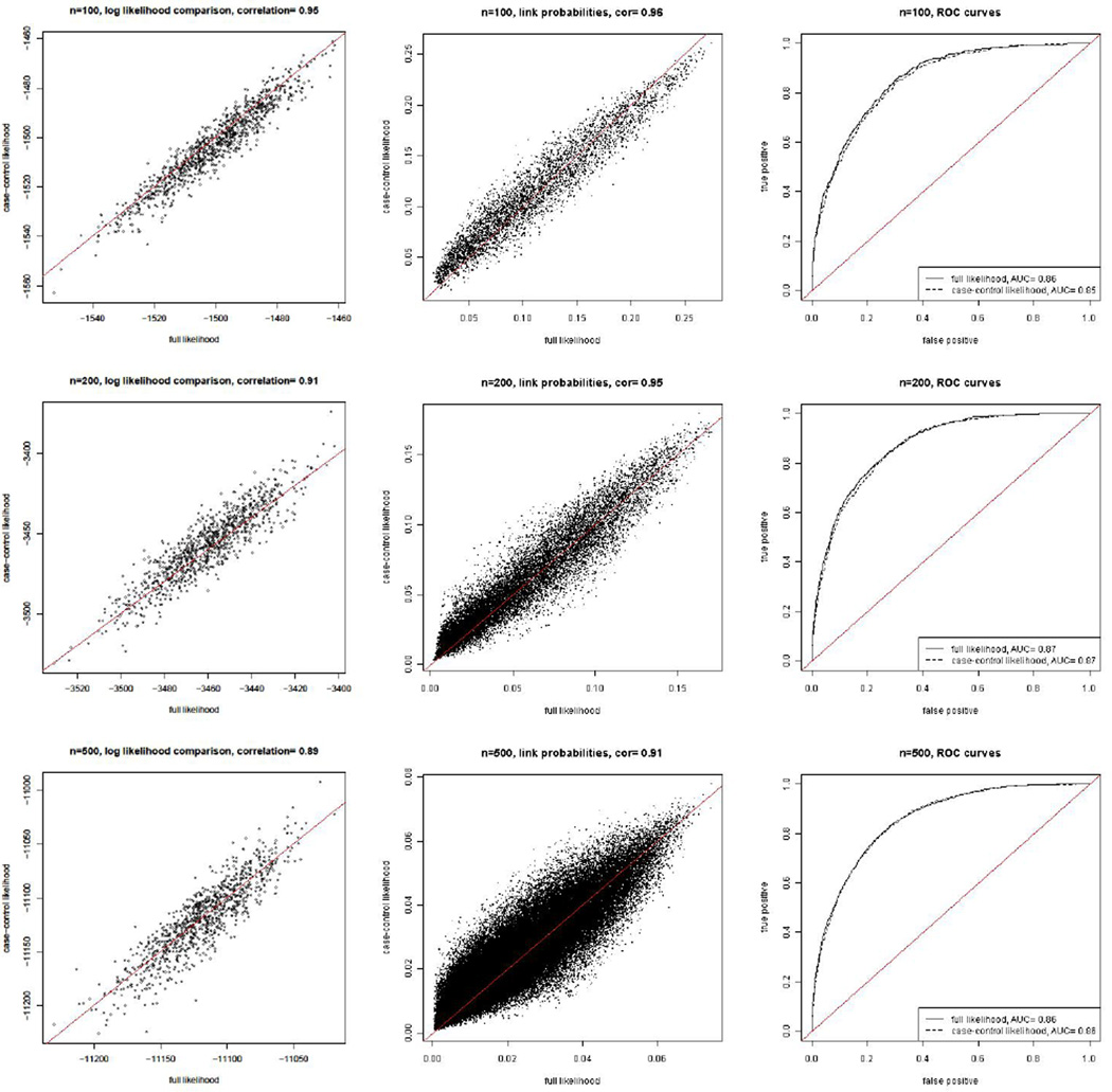
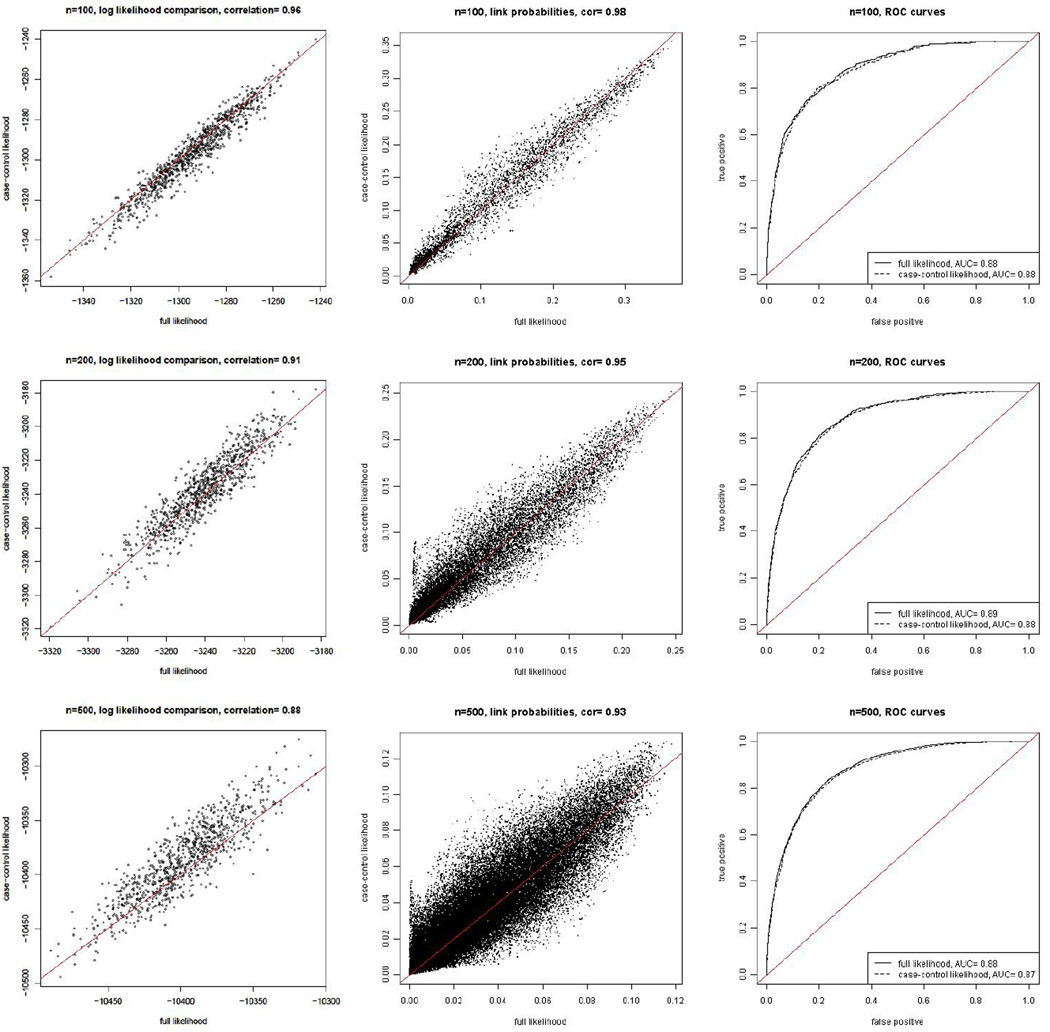
We compare the result from estimating the models using Bayesian MCMC with the case-control likelihood and the full likelihood in Figure 1 for the latent space model and Figure 2 for the latent position cluster model with two clusters.

Figure 1.

Comparison of the results using the exact likelihood with those using the case-control approximate likelihood for the latent space model with network sizes 100 (top row), 200 (middle row), and 500 (bottom row). The left panels show the exact log likelihood function on the x-axis and the case-control approximate log likelihood function on the y-axis; each point corresponds to one of the parameter vectors visited by the MCMC algorithm. The panels in the middle column show the estimated link probabilities estimated from the two likelihoods, with the the exact log likelihood function on the x-axis and the case-control approximate log likelihood function on the y-axis; each point corresponds to one directed pair of actors in the network. The right panels show the ROC curves generated by the estimated probabilities from the exact and approximate approaches; in each case these are almost identical.

Figure 2.

Comparison of the results using the exact likelihood with those using the case-control approximate likelihood for the latent position cluster model with two clusters. The panels are as described in Figure 1.

The log likelihoods from the case-control method track the full log likelihood well, as indicated by the left-most panels in Figures 1 and 2. In all cases the correlations between the two log likelihoods across values of the parameters visited by the MCMC algorithm were at least 0.88.

The fitted link probabilities using the case-control likelihood are similar to those estimated by the full likelihood, as shown by the middle columns of plots in Figures 1 and 2. The scatter plots are symmetric around the diagonal line, which is in line with the fact that the case-control log likelihood is an unbiased estimator of the full log likelihood. The link probabilities estimated by the two methods are highly correlated, with correlations of 0.96 for N = 100 and 200, and 0.91 for N = 500. The lower correlation for N = 500 is not of great concern, because the log likelihood itself is based on an average of components based on the different links. When N is larger the average involves more links, reducing the variation in individual components more.

The ROC curves generated by the case-control likelihood are indistinguishable from those generated by the full likelihood, as shown by the right-most plots in Figures 1 and 2. This indicates that the two estimation methods provide essentially identical overall fits to the data in terms of predicting links.

4 Protein-Protein Interaction Data

Protein-protein interactions (PPI) are important for many biological processes, and understanding such networks can give insights into the function of individual proteins, protein complexes and cellular machinery (Uetz et al. 2000, Kuchaiev et al. 2009). A PPI network is an undirected graph in which the nodes are proteins and two proteins are linked by an edge if they interact. Most information about PPI comes from high throughput experiments such as yeast two-hybrid or tandem affinity purification. These high throughput techniques are known to produce many false positives and false negatives. For example, the false positive rates could be as high as 64% for yeast two-hybrid experiments and 77% for tandem affinity purification experiments (Edwards et al. 2002). These false positive links can yield misleading scientific hypotheses and lead to costly and unproductive biological validation experiments. Hence, there is great interest in finding ways to identify and remove these false positive links (Mahdavi and Lin 2007; Kuchaiev et al. 2009).

Here, we use the PPI data for the yeast Saccharomyces cerevisiae as an example of the usefulness of the latent space model. The latent space model assumes that the presence of a link depends on the distance between the latent positions of two nodes. One possible use of the latent space model is to help identify the false positive links in the PPI network. We downloaded the PPI data from the Saccharomyces Genome Database (SGD) (http://downloads.yeastgenome.org) compiled from the Biological General Repository for Interaction Datasets (BioGRID) database (Stark et al. 2006). In Section 4.1, we show that our approximate casecontrol likelihood yields similar results to the full likelihood using a small random subnetwork. In Section 4.2, we show the effectiveness of the latent space model in identifying false positives in a large PPI network.

4.1 A randomly selected small subset of the PPI data

Our previous simulation results show that when the data are generated from a latent space model, the case-control approximation can provide similar estimation to the full likelihood. These results are based on simulated networks from the latent space and latent position cluster models, when we know that the model we fit is the correct one. Before applying the case-control likelihood approximation to the full data, we would like to evaluate the performance of the case-control likelihood for this real data set, when we do not know the true model and so there may be lack of fit.

We selected a connected subnetwork with 200 nodes and 1524 links, counting the symmetric pairs twice. For this sub-network we were able to fit the latent space model using the full likelihood and to compare the results with those using the case-control likelihood. We fit the latent space model using both the exact likelihood and the case-control approximation, and we evaluated the case-control approximation in a similar manner to how we did it in Section 3. The results are summarized in Figure 3. The results from fitting the subnetworks show that the case-control likelihood works well for the real data too.

Figure 3.

Comparison of the results using the exact likelihood with those using the case-control approximation for the PPI sub-network of size 200. The panels are as described in Figure 1.

In order to evaluate whether we can identify false positive links, we randomly implanted false positives by adding about 150 non-existent edges to the PPI data. This increases the number of links by about 20%. Then we fit the latent space model to this perturbed dataset using both the full likelihood and the case-control approximate likelihood to see whether we are able to identify the false links.

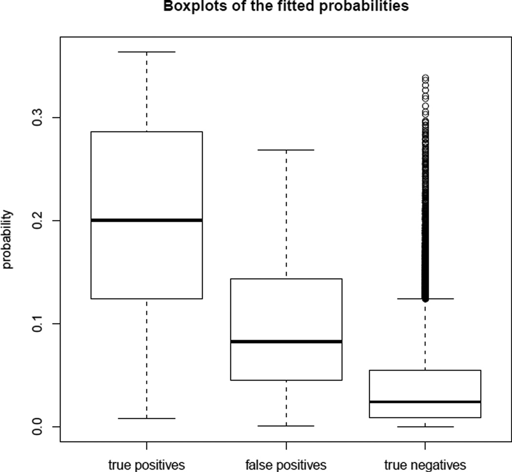
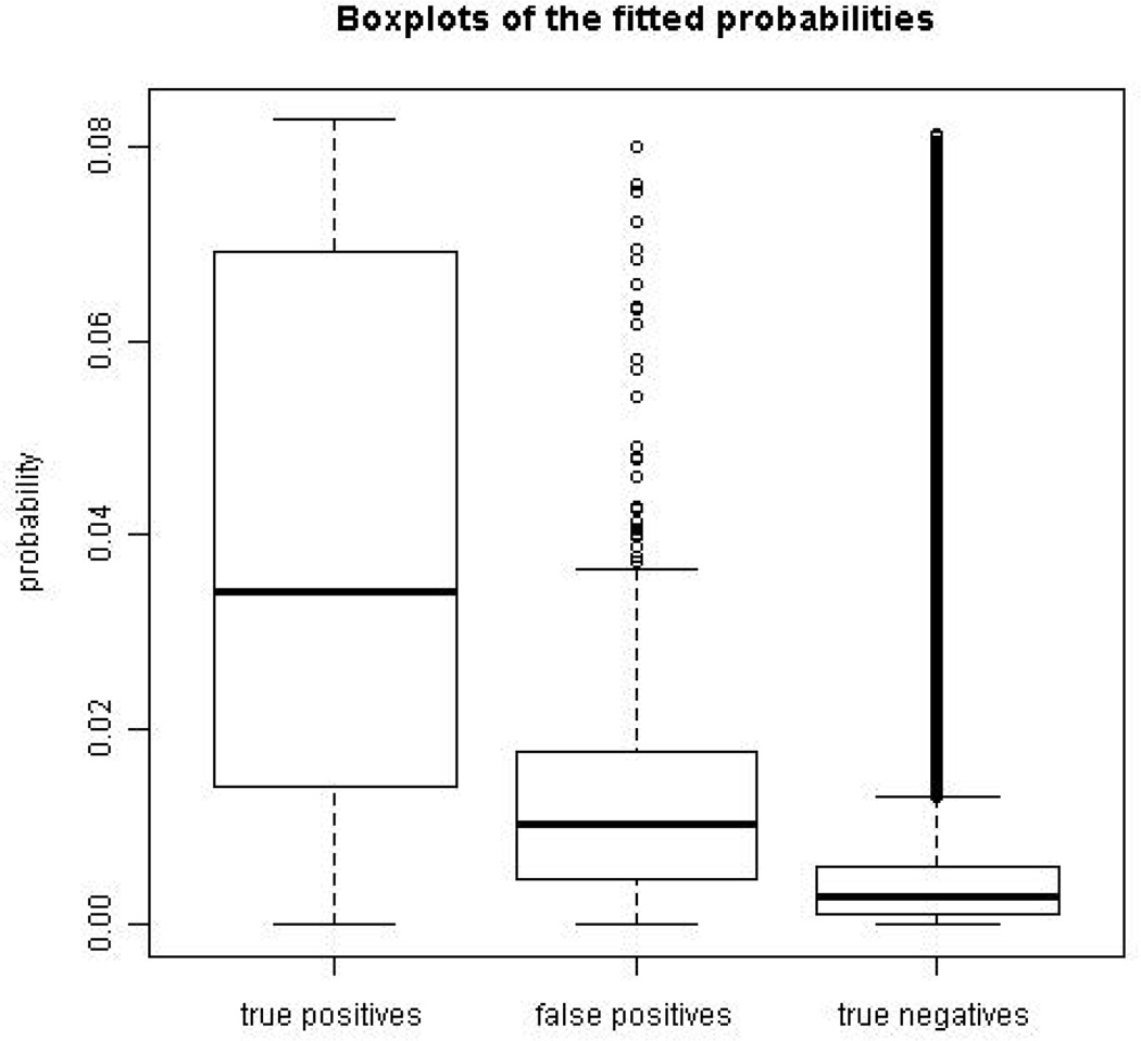
The case-control likelihood and the full likelihood produced similar results. Among the fitted probabilities for the perturbed data, the nine smallest probabilities were from the false positives, and 26 of the 50 smallest probabilities were from false positives. The boxplots of the fitted probabilities of the true positives, false positives, and true negatives in Figure 4 indicate that the false positives had much lower fitted probabilities of being links than the true positives on average. These results suggest that the latent space network model is potentially useful for identifying false positive links in PPI network data, and that its usefulness is not diminished by using the much more computationally efficient case-control approximation.

Figure 4.

Perturbed PPI sub-network of size 200: boxplots of the fitted probabilities of the true positives (left), false positives (middle), and true negatives (right).

4.2 A large PPI dataset

4.2.1 Visualization of the PPI data

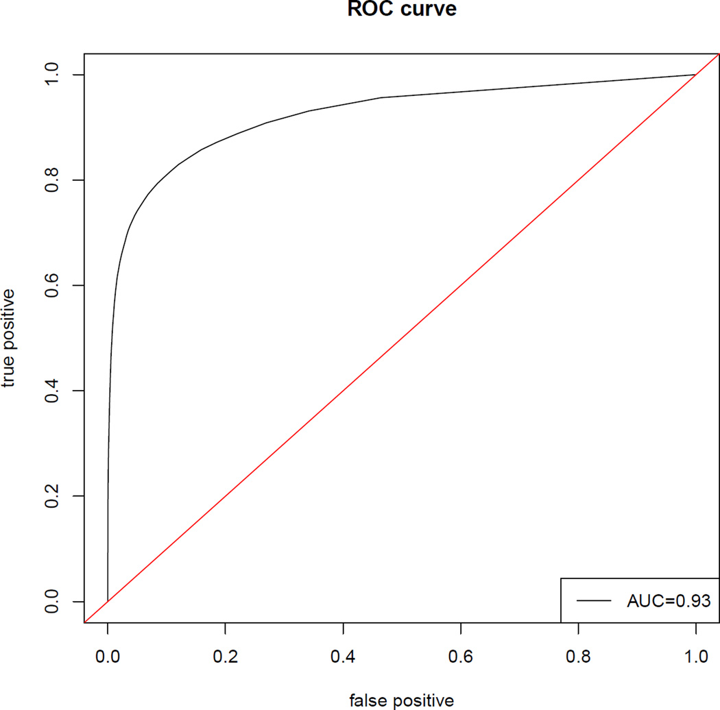
The large PPI physical interaction network we are using has 2,716 proteins with a total of 27,586 links, where the symmetric pairs have been counted twice. This is a sparse network with a mean degree of about 10 links per protein, and a median degree of only 5. This discrepancy between the mean and median indicates different activity levels across the nodes. The most active protein has 194 links while 495 proteins have only one link and a quarter of the proteins have 2 links. Figure 5 plots the ROC curve constructed by the fitted probabilities, which suggests that the latent space model fits the data reasonably well.

Figure 5.

ROC curve of the fitted link probabilities for the large PPI dataset.

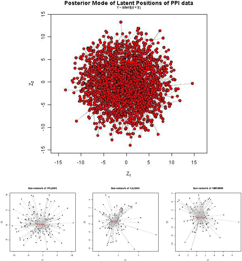
One advantage of the latent space model is that it provides a visualization of the network data. We plot the latent positions of all of the proteins in Figure 6. The large number of proteins makes it hard to see detail in this plot. To illustrate the visualization of parts of the network, we chose three of the most active proteins, and zoomed in to the three subnetworks, each of which consisted of one of the most active proteins and the other proteins that have links to it. These three subnetworks are shown in the bottom panel of Figure 6.

Figure 6.

Latent positions for the large PPI dataset (top panel), and subnetworks of the three most active proteins (bottom 3).

4.2.2 Identifying false positive links

Similarly to what we did for the subset of the data, we first randomly perturbed the data by changing a number of 0’s into 1’s equal to 20% of the number of actual links in the original dataset. We then fit the latent space model to this perturbed dataset. The boxplots of the fitted probabilities of the true positives, false positives, and true negatives in Figure 7 indicate that the fitted probabilities for the false positives were much lower than those for the true positives, and indeed were closer on average to those for the true negatives. Eight of the 10 smallest fitted link probabilities were from the false positives. These results for the full dataset suggest that the latent space model may provide a promising way to identify false positive links. Note that these results were obtained using the case-control approximate likelihood only.

Figure 7.

Perturbed full PPI data: boxplots of the fitted probabilities of the true positives (left), false positives (middle), and true negatives (right).

Next we used the fitted link probabilities from the real data to identify false positive links. We would suspect that those links in the data with very low fitted probabilities are probably false positive links. Mahdavi and Lin (2007) used Gene Ontology (GO) annotations to reduce false positive protein-protein interactions (PPI) pairs resulting from computational predictions. The key idea is that interacting proteins are likely to share GO slim terms. We used this criterion to evaluate the fitted link probabilities we get from the latent space model. We used the GO-slim terms (Ashburner et al. 2000) from the SGD database (http://downloads.yeastgenome.org). For each pair of interacting proteins, if it is documented to share one or more GO slim terms, we called it a true positive, otherwise a false positive. Note that this definition of true and false positives is itself subject to error.

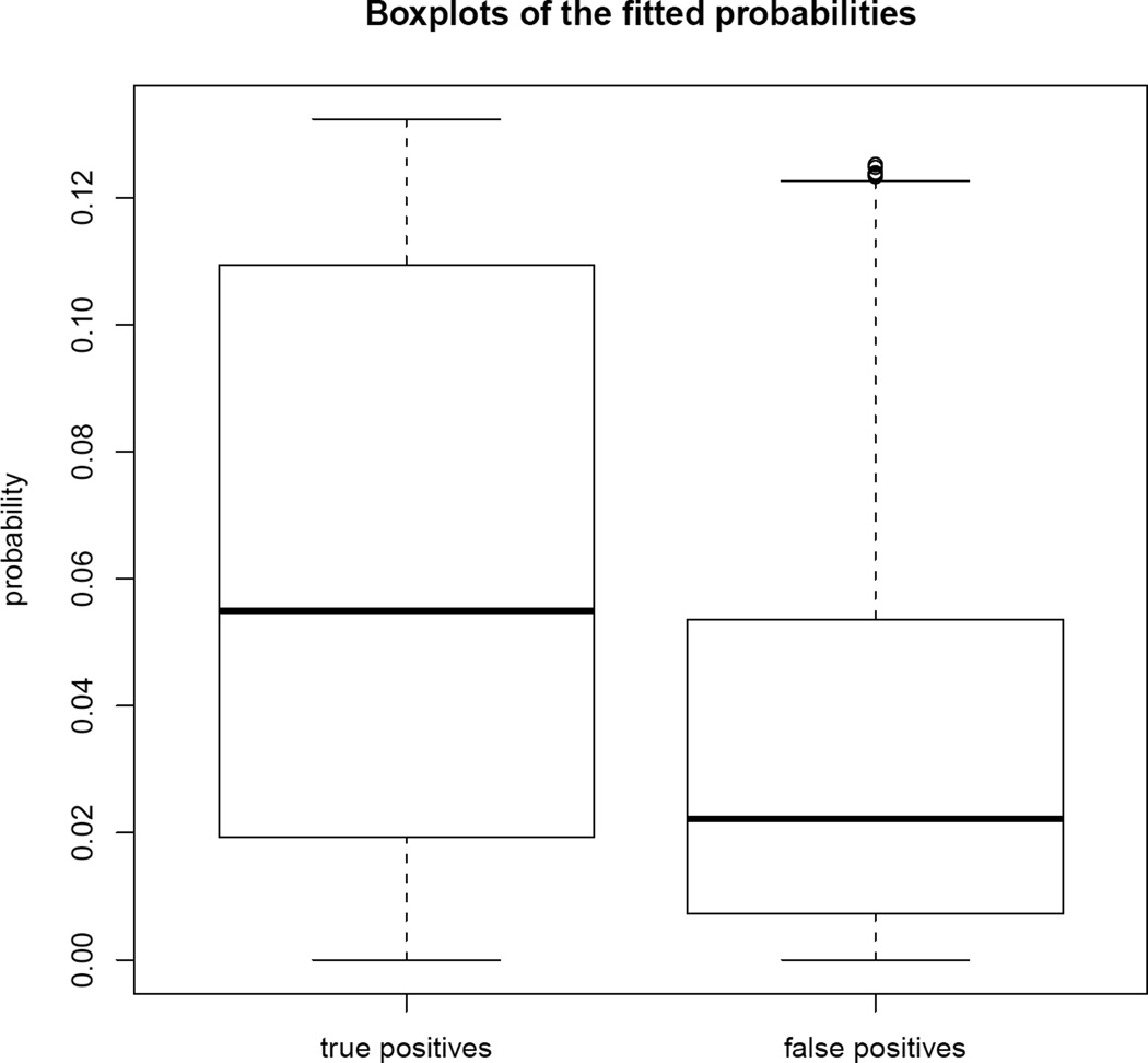
We compare the boxplots of the fitted link probabilities of the true positives and false positives in Figure 8. We can clearly see a difference in the two populations, which indicates that there is considerable agreement between the identification of false positives by the latent space model and by the GO-slim terms. Of course we would not expect perfect or even very strong agreement, even if the latent space model discriminated perfectly between true and false positives, because the GO-slim terms provide only an imperfect measurement of false positives.

Figure 8.

Real full PPI data: fitted link probabilities grouped by whether or not the edges share a GO-slim term

5 Discussion

An obstacle to the use of latent space models for networks has been the fact that existing likelihood and Bayesian estimation methods do not scale to large networks, because the required computation is O(N²), where N is the number of nodes or actors in the network. We have proposed an approximate likelihood based on the same idea that underlies case-control studies, and we have found it to perform well in simulated and real data. This reduces computation from O(N²) to O(N), and makes it feasible to do Bayesian estimation via MCMC for large networks.

We have implemented our method for estimating the latent space model (Hoff et al. 2002) and the latent position cluster model (Handcock et al. 2007), but the basic idea can be applied to other statistical network models as well. They can be used to reduce computation for likelihood-based estimation for network models for which the log likelihood involves a sum of contributions from all or most of the pairs of actors. These include the latent position random effects model (Krivitsky et al. 2009), which is a direct extension of the latent space, and explicitly models different activity levels of nodes. They also include the latent class model of Nowicki and Snijders (2001) and the latent factor model of Hoff et al. (2002). See Goldenberg et al. (2009) for a survey of these and other network models.

Other approaches to efficient computation for statistical network models have been explored, notably the variational Bayes approach of Attias (1999). This was applied to stochastic blockmodels by Airoldi et al. (2008) and extended to the latent position cluster model by Salter-Townshend and Murphy (2010). Rather than try to approximate the likelihood, this attempts to find and use a lower bound for the likelihood.

References

- Airoldi EM, Blei DM, Fienberg SE, Xing EP. Mixed membership stochastic blockmodels. Journal of Machine Learning Research. 2008;9:1981–2014. [PMC free article] [PubMed] [Google Scholar]
- Ashburner M, Ball CA, Blake JA, Botstein D, Butler M, Cherry JM, Davis AP, Dolinsky K, Dwight SS, Eppig JT, Harris MA, Hill DP, Issel-Tarver L, Kasarskis A, Lewis S, Matese JC, Richardson JE, Ringwald M, Rubin GM, Sherlock G. Gene ontology: tool for the unification of biology. the gene ontology consortium. Nature Genetics. 2000;25:25–29. doi: 10.1038/75556. [DOI] [PMC free article] [PubMed] [Google Scholar]
- Attias H. Inferring parameters and structure of latent variable models by Variational Bayes; Proceedings of the Fifteenth Conference on Uncertainty in Artificial Intelligence; 1999. pp. 21–30. [Google Scholar]
- Barabási AL, Oltvai ZN. Network biology: Understanding the cell's functional organization. Nature Reviews Genetics. 2004;5:101–113. doi: 10.1038/nrg1272. [DOI] [PubMed] [Google Scholar]
- Breslow NE. Statistics in epidemiology: The case-control study. Journal of the American Statistical Association. 1996;91:14–28. doi: 10.1080/01621459.1996.10476660. [DOI] [PubMed] [Google Scholar]
- Breslow NE, Day N. Statistical Methods in Cancer Research, Vol 1: The Analysis of Case-control Studies. Lyon: IARC Scientific Publications; 1980. [PubMed] [Google Scholar]
- Edwards AM, Kus B, Jansen R, Greenbaum D, Greenblatt J, et al. Bridging structural biology and genomics: assessing protein interaction data with known complexes. Trends in Genetics. 2002;18:529–536. doi: 10.1016/s0168-9525(02)02763-4. [DOI] [PubMed] [Google Scholar]
- Frank O, Strauss D. Markov graphs. Journal of the American Statistical Assiciation. 1986;81:832–842. [Google Scholar]
- Goldenberg A, Zheng AX, Fienberg SE, Airoldi EM. A survey of statistical network models. Foundations and Trends in Machine Learning. 2009;2:129–233. [Google Scholar]
- Handcock MS, Raftery AE, Tantrum JM. Model-based clustering for social networks (with discussion) Journal of the Royal Statistical Society, Series A. 2007;170:301–354. [Google Scholar]
- Hoff PD. Multiplicative latent factor models for description and prediction of social networks. Computational and Mathematical Organization Theory. 2009;15:261–272. [Google Scholar]
- Hoff PD, Raftery AE, Handcock MS. Latent space approaches to social network analysis. Journal of the American Statistical Association. 2002;97:1090–1098. [Google Scholar]
- Krivitsky P, Handcock MS, Raftery AE, Hoff PD. Representing degree distributions, clustering, and homophily in social networks with latent cluster random ects models. Social Networks. 2009;31:204–213. doi: 10.1016/j.socnet.2009.04.001. [DOI] [PMC free article] [PubMed] [Google Scholar]
- Kuchaiev O, Rašajski M, Higham DJ, Pržulj N. Geometric denoising of protein-protein interaction networks. PLoS Computational Biology. 2009;5:e1000454. doi: 10.1371/journal.pcbi.1000454. [DOI] [PMC free article] [PubMed] [Google Scholar]
- Mahdavi MA, Lin Y-H. False positive reduction in protein-protein interaction predictions using gene ontology annotations. BMC Bioinformatics. 2007;8:262. doi: 10.1186/1471-2105-8-262. [DOI] [PMC free article] [PubMed] [Google Scholar]
- McFarland DD, Brown DJ. Social distance as a metric: A systematic introduction to smallest space analysis. In: Laumann E, editor. Bonds of Pluralism: The Form and Substance of Urban Social Networks. New York: Wiley; 1973. pp. 213–253. [Google Scholar]
- Nowicki K, Snijders TAB. Estimation and prediction for stochastic block-structures. Journal of the American Statistical Association. 2001;96:1077–1087. [Google Scholar]
- Salter-Townshend M, Murphy TB. Technical report. School of Mathematical Sciences, University College Dublin; 2010. Variational Bayesian inference for the latent position cluster model. [Google Scholar]
- Stark C, Breitkreutz BJ, Reguly T, Boucher L, Breitkreutz A, Tyers M. Biogrid: A general repository for interaction datasets. Nucleic Acids Research. 2006;34:D536–D539. doi: 10.1093/nar/gkj109. [DOI] [PMC free article] [PubMed] [Google Scholar]
- Uetz P, et al. A comprehensive analysis of protein-protein interactions in Saccharomyces cerevisiae. Nature. 2000;403:623–627. doi: 10.1038/35001009. [DOI] [PubMed] [Google Scholar]
- Wang YJ, Wong GY. Stochastic blockmodels for directed graphs. Journal of the American Statistical Association. 1987;82:8–19. [Google Scholar]
- Wasserman S, Pattison P. Logit models and logistic regressions for social networks: I. An introduction to markov graphs and p*. Psychometrika. 1996;61:401–425. [Google Scholar]